LEABHARLANN CHOLAISTE NA TRIONOIDE, BAILE ATHA CLIATH TRINITY COLLEGE LIBRARY DUBLIN OUscoil Atha Cliath The University of Dublin
Terms and Conditions of Use of Digitised Theses from Trinity College Library Dublin Copyright statement
All material supplied by Trinity College Library is protected by copyright (under the Copyright and Related Rights Act, 2000 as amended) and other relevant Intellectual Property Rights. By accessing and using a Digitised Thesis from Trinity College Library you acknowledge that all Intellectual Property Rights in any Works supplied are the sole and exclusive property of the copyright and/or other I PR holder. Specific copyright holders may not be explicitly identified. Use of materials from other sources within a thesis should not be construed as a claim over them.
A non-exclusive, non-transferable licence is hereby granted to those using or reproducing, in whole or in part, the material for valid purposes, providing the copyright owners are acknowledged using the normal conventions. Where specific permission to use material is required, this is identified and such permission must be sought from the copyright holder or agency cited.
Liability statement
By using a Digitised Thesis, I accept that Trinity College Dublin bears no legal responsibility for the accuracy, legality or comprehensiveness of materials contained within the thesis, and that Trinity College Dublin accepts no liability for indirect, consequential, or incidental, damages or losses arising from use of the thesis for whatever reason. Information located in a thesis may be subject to specific use constraints, details of which may not be explicitly described. It is the responsibility of potential and actual users to be aware of such constraints and to abide by them. By making use of material from a digitised thesis, you accept these copyright and disclaimer provisions. Where it is brought to the attention of Trinity College Library that there may be a breach of copyright or other restraint, it is the policy to withdraw or take down access to a thesis while the issue is being resolved.
Access Agreement
By using a Digitised Thesis from Trinity College Library you are bound by the following Terms & Conditions. Please read them carefully.
Short-Term Traffic Condition
Variables Forecasting using Artificial
Neural Networks
by
STEPHEN DUNNE
A dissertation submitted to the University of Dublin in the partial fulfilment of
the requirements for the Degree of Doctor of Philosophy
Department of Civil, Structural and Environmental Engineering
DECLARATION
I declare that this thesis has not been submitted as an exercise for a degree at this or any other
university and it is entirely my own work.
I agree to deposit this thesis in the University’s open access institutional repository or allow the
library to do so on my behalf, subject to Irish Copyright Legislation and Trinity College Library
conditions of use and acknowledgement.
JTRINITY COLLEGE
- 4 MAR 20U
LIBRARY DUBLIN ^DEDICATION
SUMMARY
Short-term traffic forecasting (STTF) is a critical element of Intelligent Transport Systems
(ITS). The use of ITS is vital in order to ensure the sustainability and increase the efficiency of
the transportation network. ITS bases decisions on traffic conditions and so it can only be
effective if the forecasted future traffic conditions provided are accurate. There exists multiple
STTF algorithms, of which Artificial Neural Networks (ANNs) are the predominant non-
parametric approach. Prediction of traffic variables using ANN is a well-researched area
(Karlaftis & Vlahogianni, 2011) and the different structures and applications of ANN in traffic
forecasting have established the strength of these models compared to other existing
methodologies. Due to their ability of precise predictions, adaptability, flexibility and
availability of numerous software, ANN models are the focus of this thesis from the outset,
while other models are used for accuracy comparisons The research in this dissertation focused
on adapting and improving further the ANN based STTF algorithms for predicting traffic
conditions in more complex paradigms.
The input vectors to ANN algorithms and the learning rules employed within the
network structure have been optimised for improving efficiency of traditional ANN algorithms
in STTF literature. In the literature there are arguments for the use of reasonably short intervals
(15 minutes) as traffic flow fluctuates over short time intervals and this suggests a loss of
information when using coarser time aggregations. By forecasting data at different time
aggregations in this work, conclusions could be drawn on which time aggregation is the most
sensible based on the forecasting results.
traffic condition variables separately under congested and uncongested regimes. The
relationship between traffic speed and flow was utilised in identifying the congestion levels,
with flow and speed having a linear relationship in the uncongested regime and a non-linear
relationship in the congested regime. The multivariate algorithm predicted both speed and flow
in near future.
One of the major contributions of this thesis involved the use of rainfall as an
exogenous variable input to ANN prediction models for predicting traffic flow. With climate
change an ever looming issue, it was important to factor in the effect of weather on traffic
conditions. This was achieved through a multivariate prediction model which made use of
rainfall as an additional model input, only when rainfall was expected in the coming prediction
interval. Rainfall does not influence traffic conditions instantaneously but it changes long term
traffic dynamics within the day. The effect of rainfall on traffic dynamics is best viewed by
looking at different frequency levels of traffic condition variable time-series. As such, another
novel feature of the work in this thesis involved the introduction of Stationary Wavelet
Transforms (SWTs) to decompose traffic flow time-series. The use of SWT decomposition
allowed the separate resolution components to be predicted separately in an effort to improve
forecasting accuracy. This was among the first uses of SWTs in the field of traffic flow
forecasting.
The ANN and SWT based weather adaptive traffic flow prediction model in this thesis
was also applied to predicting travel time. In this work, both SWT and the multivariate rainfall
approach were used to predict travel time sourced from traffic cameras on Pearse St., Dublin.
Travel times change based on driver behaviour and hence predicting a range is often more
meaningful to commuters than point forecasts. Hence, Forecast Regions (FRs) were constructed
for travel time prediction using four different approaches.
centre and forecasts were also conducted using highway data from the Motorway Incident
Detection and Automated Signalling (MIDAS) dataset in the U.K. There have been many
instances of urban arterial or highway traffic flow data forecasting but the two were rarely
compared. The differences in the traffic behaviour at each site, and the relative forecasts, were
examined. Both urban and highway datasets were used based on the scope of the different
prediction algorithms developed in this work.
ACKNOWLEDGEMENTS
I would like to express my sincere thanks to my thesis supervisor Dr. Bidisha Ghosh. Dr. Ghosh
was always available to me if I had any issues whatsoever and the conversations we had over
the course of my research were invaluable when shaping my dissertation. Her wealth of
knowledge regarding my field was also a huge help to me when I had queries about specific
models.
I would like to thank Dr. Kevin Ryan of the Civil, Structural and Environmental
Engineering Department in Trinity College for all his help in the lab and on site, particularly
with the ANPR cameras and storage media. Also, the people at DCC, particularly Brian Carrig
and Gary Keegan, were a great help with obtaining data and getting the ANPR cameras set up. I
would also like to thank the staff of the Austrian Institute of Technology in Vienna, especially
Bernhard Heilmann, who shared their data with me and made me feel very at home during my
working visit.
I would also like to thank my girlfriend Nicole who helped me through my four years of
research. She was always there to spend time with me when a break from the research was
needed and she supported and encouraged me from day one. She understood how much of a
time commitment was required to complete postgraduate research and always encouraged me to
spend as much time on my work as was needed.
Thirdly, I would like to thank my family for being a constant source of encouragement
throughout my four years of postgraduate research. With the help of their constant support, the
research was never allowed to get on top of me. It was always enjoyable to relax after a long
day of research by spending time with my family.
TABLE OF CONTENTS
DECLARATION
DEDICATION
SUMMARY
ACKNOWLEDGEMENTS
TABLE OF CONTENTS
LIST OF FIGURES
LIST OF TABLES
LIST OF ACRONYMS
1
Chapter 1
1.1
Background
1.2
Literature Review
2
Chapter 2
2.1
Introduction
2.2
Methodology
2.2.1
Feed Forward Back Propagation Neural Network
2.2.2
Radial Basis Function Neural Network
2.2.3
Generalized Regression Neural Network
2.2.4
Support Vector Machine
2.2.5
Autocorrelation Neural Network (ACNN)
2.3
Traffic Flow Data
2.3.1
Urban Arterial Traffic Flow Data
2.3.2
Motorway Traffic Flow Data
2.4
Results
2.4.1
Artificial Neural Network and Support Vector Machine Modelling Setup
2.4.2
Comparison of Predictions
2.5
Conclusion
3
Chapter 3
3.1
Introduction
3.2
Methodology
3.2.1
Regime Isolation Methodology
3.2.2 ACNN with Various Learning Rules 81
3.3 Application of the proposed Prediction Algorithm 83
3.3.1 Traffic Data 83
3.3.2 Model Fitting 87
3.4 Forecasts 89
3.5 Conclusion 96
4 Chapter 4 98
4.1 Introduction 98
4.2 Methodology 99
4.2.1 Stationary Wavelet Transform 100
4.2.2 Neuro-Wavelet Prediction Framework 103
4.3 Evaluation of Neuro-Wavelet Model 106
4.3.1 Data 106
4.3.2 Traffic modelling using SWT-ACNN Structure 109
4.4 Prediction and Comparisons 113
4.5 Conclusion 115
5 Chapter 5 117
5.1 Introduction 117
5.2 Summary of Travel Time Data Collection Methods 117
5.3 Case Study 1: Dublin Automatic Number Plate Recognition (ANPR) Camera Dataset 120
5.3.1 Camera and eBox Description 121
5.3.2 Data Software Interface and Travel Time Dataset Creation 128
5.4 ANPR Travel Time Data Description 132
5.4.1 Pearse St. Travel Time Dataset 132
5.4.2 Tallaght Travel Time Dataset 133
5.5 Case Study 2: Vienna Probe Vehicle Travel Time Dataset 136
5.6 Conclusion 138
6 Chapter 6 140
6.1 Introduction 140
6.2 Methodology 141
6.2.1 Forecast Region Construction 142
6.2.2 Forecast Region Assessment Indices 150
6.3 Data 152
6.5
Conclusion
163
7 Chapter 7
165
7.1
Research Summary
165
7.2
Research Findings and Critical Assessments
166
7.3
Recommendations for Further Research
169
REFERENCES
171
LIST OF FIGURES
Figure 2.1: A Biological Neuron 27
Figure 2.2: A Basic Artificial Neuron 28
Figure 2.3: Basic Feed Forward Phase of a Neural Network Structure 30 Figure 2.4: Feed Forward Back Propagation Neural Network Structure 33
Figure 2.5: Radial Basis Function Neural Network 36
Figure 2.6: Generalized Regression Neural Network 38
Figure 2.7: Order of Processes 42
Figure 2.8: Map of Urban Arterial Junctions 44
Figure 2.9: Typical Hourly Traffic Flow at Junctions TCS 141, TCS 166 and TCS 183 45 Figure 2.10: Correlograms of (a) Non-Stationary Data & (b) Stationary Data - Junction TCS
141 47
Figure 2.11: Map of Motorway Locations 49
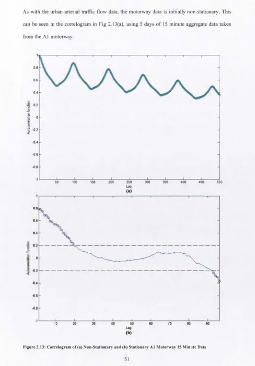
Figure 2.12: Typical Hourly Traffic Flow at the A1 and M6 Motorways 50 Figure 2.13: Correlogram of (a) Non-Stationary and (b) Stationary A1 Motorway 15 Minute
Data 51
Figure 2.14: FFBPNN Predictions at Junction TCS 141 55
Figure 2.15: FFBPNN Predictions at Junction TCS 166 56
Figure 2.16: FFBPNN Predictions at Junction TCS 183 56
Figure 2.17: FFBPNN Predictions at the A1 Motorway 57
Figure 2.18: FFBPNN Predictions at the M6 Motorway 57
Figure 2.19: RBFNN Predictions at Junction TCS 141 58
Figure 2.20: RBFNN Predictions at Junction TCS 166 58
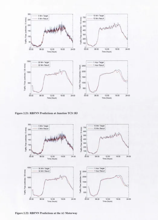
Figure 2.21: RBFNN Predictions at Junction TCS 183 59
Figure 2.22: RBFNN Predictions at the A1 Motorway 59
Figure 2.23: RBFNN Predictions at the M6 Motorway 60
Figure 2.24: GRNN Predictions at Junction TCS 141 60
Figure 2.25: GRNN Predictions at Junction TCS 166 61
Figure 2.26: GRNN Predictions at Junction TCS 183 61
Figure 2.27: GRNN Predictions at the A1 Motorway 62
Figure 2.28: GRNN Predictions at the M6 Motorway 62
Figure 2.29: SVM Predictions at Junction TCS 141 63
Figure 2.30: SVM Predictions at Junction TCS 166 63
Figure 2.31: SVM Predictions at Junction TCS 183 64
Figure 2.33: SVM Predictions at the M6 Motorway
65
Figure 2.34: MAPE vs. Time Aggregation Subplot
67
Figure 2.35: FFBPNN TCS 141 15 Minute Data - ACF vs. Non-ACF Predictions
71
Figure 2.36: TCS 141 Predictions - ACNN vs. Naive Method vs. Moving Average
72
Figure 3.1: Flow Diagram for the Multivariate Prediction Methodology
78
Figure 3.2: (a) Flow-Speed Scatterplot & (b) Difference of Slope Graph
79
Figure 3.3: Weekday 15 Minute Aggregate Traffic Flow
84
Figure 3.4: Weekday 15 Minute Aggregate Average Speed
85
Figure 3.5: Flow-Speed Scatterplots for the 4 Lanes
87
Figure 3.6: Prediction Results for 15 Minute Time Aggregations using ALRLM at Lane 1 of
A1/9340A
94
Figure 3.7: Prediction Accuracy vs. Time Aggregations using ALRLM for 4 Motorway Lanes
95
Figure 4.1: Stationary Wavelet Transform Decomposition Tree
102
Figure 4.2: Stationary Neuro-Wavelet Prediction Framework
104
Figure 4.3: Location of SCATS Data Collection Sites
107
Figure 4.4: Typical Weekday Flourly Traffic Flow Data
108
Figure 4.5: Barchart of Hourly Rainfall Data for the first 10 Weekdays of 2009
109
Figure 4.6: Hourly Traffic Flow db3 Wavelet Decomposition
111
Figure 4.7: TCS 106 Prediction Results
113
Figure 4.8: TCS 125 Prediction Results
114
Figure 5.1: Travel Time Dataset Creation Flow Chart
120
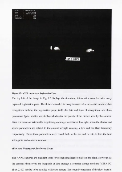
Figure 5.2: ANPR capturing a Registration Plate
122
Figure 5.3: ANPR Camera and Waterproof Box
123
Figure 5.4: Schematics of Waterproof Box
124
Figure 5.5: Overview of ANPR Camera Sites
126
Figure 5.6: ANPR Site 1 Camera Locations
127
Figure 5.7: ANPR Site 2 Camera Locations
127
Figure 5.8: FTP Settings on ANPR Camera
129
Figure 5.9: Pearse St. 15 Minute Aggregated Average Travel Time Example
132
Figure 5.10: Location of ANPR Cameras in Tallaght
134
Figure 5.11: Tallaght Daily Travel Time Example (15 Minute Aggregation)
135
Figure 5.12: Schoenbrunnerstrasse as part of the Vienna free speed map
136
Figure 5.13: Schoenbrunnerstrasse Daily Travel Time Example (15 Minute Aggregation) 137
Figure 6.1: Average Travel Time in 15 Minute Intervals from 08:00 - 20:00 hours
152
Figure 6.2: Rainfall Barchart for 08:00 hours to 20:00 hours from July 30th to August 3rd 2012
Figure 6.3: FR generated using the Bootstrap Method Figure 6.4: FR generated using the Delta Method
Figure 6.5: FR created using Bayesian Hierarchical Interval Estimation
Figure 6.6: Standard Nonconformity Measure ICP Based FR Construction Method Figure 6.7: Normalised Nonconformity Measure ICP Based FR Construction
LIST OF TABLES
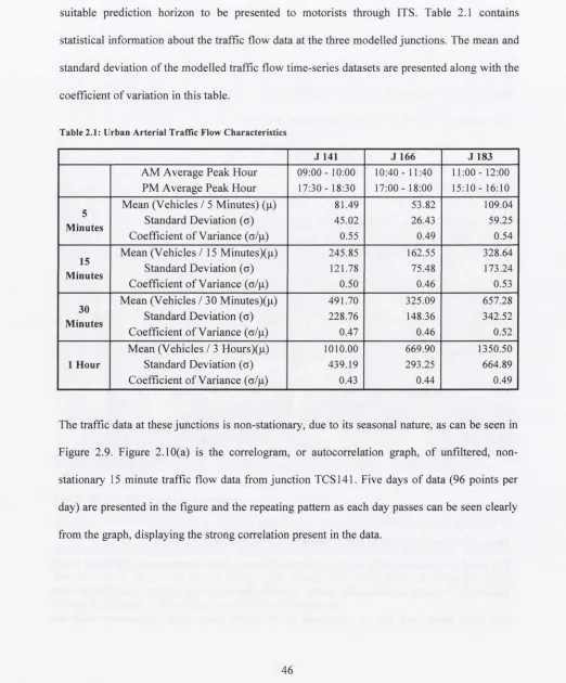
Table 2.1: Urban Arterial Traffic Flow Characteristics
46
Table 2.2: Urban Arterial Influential Points based on Correlograms
48
Table 2.3: Motorway Traffic Flow Characteristics
50
Table 2.4: Motorway Data Influential Points based on Correlograms
52
Table 2.5: Prediction Results - MAPE (%) and RMSE
66
Table 2.6: Computational Time for the Prediction Models
69
Table 2.7: ACF vs. Non-ACF Prediction Error Values
71
Table 2.8: TCS 141 15 Min Predictions- ACNN vs. Naive Model vs. MA technique
73
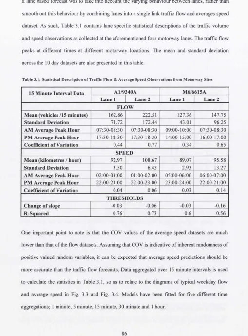
Table 3.1: Statistical Description of Traffic Flow & Average Speed Observations from
Motorway Sites
86
Table 3.2: Traffic Flow Prediction Results
91
Table 3.3: Average Traffic Speed Prediction Results
92
Table 4.1: TCS 106 Rainfall Data Correlation Coefficients
112
Table 4.2: Prediction Accuracies at TCS 106 and TCS 125 under different Weather Conditions
115
Table 5.1: Pearse St. Travel Time Dataset Descriptive Statistics
133
Table 5.2: Tallaght Travel Time Dataset Descriptive Statistics
135
Table 5.3: Schoenbrunnerstrasse Travel Time Dataset Descriptive Statistics
138
Table 6.1: Travel Time Dataset Descriptive Statistics
153
Table 6.2: Travel Time Prediction Results
154
LIST OF ACRONYMS
ACF
Autocorrelation Function
ACNN
Autocorrelation Neural Network
ACO
Ant Colony Optimisation
ALRLM
Levenberg-Marquardt Model
ALRM
Adaptive Learning Rate Model
ALRMM
Adaptive Learning Rate with Momentum Model
ANN
Artificial Neural Network
ANPR
Automatic Number Plate Recognition
ARIMAAutoregressive Integrated Moving Average
ARIMAXAutoregressive Integrated Moving Average Errors
AXISAdvanced Traveller Information System
ATMS
Advanced Traffic Management System
AVD
Alpha Vision Design
BHIE
Bayesian Hierarchical Interval Estimation
BP
Back Propagation
BPNN
Back Propagation Neural Network
CCTV
Closed Circuit Television
CLC
Coverage Length-based Criterion
COV
Coefficient of Variation
CP
Conformal Prediction
DCC
Dublin City Council
DWT
Discrete Wavelet Transform
EMD
Empirical Mode Decomposition
ERM
Empirical Risk Minimisation
FF
Feed Forward
FFBPNN
Feed Forward Back Propagation Neural Network
FNN
Fuzzy Neural Network
FR
Forecast Region
FRBS
Fuzzy Rule-Based System
FRCP
Forecast Region Coverage Probability
FTP
File Transfer Protocol
GA
Genetic Algorithm
GD
Gradient Descent
GPS
Global Positioning Systems
GRNN
Generalized Regression Neural Network
HA
Historical Average
k-NN
k-Nearest Neighbours
KF
Kalman Filter
LBS
Location Based Sensor
LM
Levenberg-Marquardt
LS
Least Squares
ICP
Inductive Conformal Prediction
IP
Internet Protocol
ISWT
Inverse Stationary Wavelet Transform
ITS
Intelligent Transportation Systems
MAPE
Mean Absolute Percentage Error
MCMC
Markov Chain Monte Carlo
MFRL
Mean Forecast Region Length
MIDAS
Motorway Incident Detection and Automated Signalling
MLP
Multi-Layer Perceptron
MNN
Modular Neural Network
MSE
Mean Square Error
MTL
Multi Task Learning
N-ICP
ICP using a Normalised Nonconformity Measure
NLR
Non-Linear Regression
NMFRL
Normalised Mean Forecast Region Length
NN
Neural Network
PSO
Particle Swarm Optimisation
RBF
Radial Basis Function
RBFNN
Radial Basis Function Neural Network
RCBO
Residual Current Circuit Breaker with Overcurrent Protection
RGS
Route Guidance Systems
RMSE
Root Mean Square Error
RNN
Recurrent Neural Network
SCATS
Sydney Coordinated Adaptive Traffic System
SDCC
South Dublin County Council
SHW
Seasonal Holt-Winters
S-ICP
ICP using a Standard Nonconformity Measure
SRM
Structural Risk Minimisation
SSNN
State Space Neural Network
STM
Structural Time-series Model
STTF
Short-Term Traffic Forecasting
sv
Support Vector
SVC
Support Vector Classification
SVM
Support Vector Machine
SVR
Support Vector Regression
SWT
Stationary Wavelet Transform
U.K.
United Kingdom
VAR
Vector Autoregressive
VPH
Vehicles Per Hour
1 Chapter 1
INTRODUCTION AND LITERATURE REVIEW
1.1 Background
The process of transporting people, goods and services from one location to another has been,
and will always be, a fundamental aspect of human life. As such, different methods of
transportation have been invented, tested and accepted throughout history. Different modes of
transport have been popular at different times in the past. Air, rail and road transport have all
maintained certain popularity since their inception as transportation modes. Of these modes,
road transport is recognised as the most popular mode in modern times. However, the
popularity of road transport has put a strain on the existing road infrastructure, particularly in
highly populated urban areas. The more popular road transport becomes, the more vehicles take
to the roads around the world. Accordingly, congestion on roads is a major problem.
drops enough to prompt users to reconsider. Therefore, the method of tackling congestion with
the most promise is that of improving the performance of the transport network in situ.
The task of improving the efficiency and sustainability of the existing road network is
not a simple one. Intelligent Transportation Systems (ITS) have been devised as a means of
performing this task. ITS are a collection of applications designed to manage the traffic on the
roads at present and to ensure the highest levels of capacity on our roads are reached, all while
avoiding delays wherever possible. ITS are composed of many aspects geared towards the task
of improving network efficiency and sustainability. These aspects include intelligent traffic
signal control systems, motorway management systems, transit management systems, incident
management systems, electronic toll collection systems, electronic fare payment systems,
emergency response systems, travel information systems and route guidance systems (Khisty &
Lall, 2002). These components can all be considered to fall under two major umbrella concepts
of ITS; Advanced Traffic Management Systems (ATMS) and Advanced Traveller Information
Systems (ATIS). ATMS incorporates traffic signal monitoring and adaptive control and traffic
condition variable data recording through the use of data collectors such as inductance loop
detectors embedded in the roads. Based on the traffic state as seen by ATMS’ detectors, ATIS
gives information regarding congestion to the motorists on the roads through such media as
Variable Message Signs (VMS) above or beside roads or through the radio directly into
vehicles. It follows that ATIS needs ATMS to function efficiently in order to be effective.
Similarly, in order for ATMS to function efficiently, information about the actual and the near-
term future traffic state is critical. It is this task of accurately forecasting traffic conditions upon
which the work in this thesis is based. With this in mind, the literature review in Section 1.2
describes previous work in the field of traffic condition forecasting.
1.2 Literature Review
1992; Head, 1995). This was first noted by Cheslow et al. (1992) who surmised that “The
ability to make and continuously update predictions of traffic flows and link times for several
minutes into the future using real-time data is a major requirement for providing dynamic traffic
control”. Traffic flow prediction has thus become an active field of research over the last fifteen
years. With the increasing amount of ITS implementation globally, a vast volume of real time
traffic flow data has become available to those in traffic management positions. There are a lot
of different data collection techniques including using inductance loop detectors embedded in
the road surface which count the number of cars passing above, while more recently video
surveillance of roads and satellite imaging technology have also come into use. As the data is
now more easily available, the problem is how best to use this data to predict traffic flow at
select intervals, as ITS cannot function optimally without the ability to forecast traffic flow
volumes in the short-term.
Parametric Models
Parametric models are based on the assumption that the structure of the underlying process of a
time-series to be forecasted can be described by a few parameters. Parametric models used to
forecast short-term traffic flow in the literature include smoothing techniques, Historical
Average (HA) algorithms, auto-regressive linear processes and Kalman filtering. Examples of
each of these forecasting methodologies are discussed in the following subsections;
(a) Historical Average Algorithms
HA models simply use an average of past traffic volumes over multiple time instants to forecast
future traffic volume and consequently they rely upon the periodic nature of traffic flow.
However, there is one major flaw with this type of model i.e. the model has no way to react to
dynamic changes in the transportation system, such as collisions or oil spills etc. Due to this, the
HA forecasting model produced the largest error in a study by Smith and Demetsky (1997),
which compared the HA model with an AutoRegressive Integrated Moving Average (ARIMA)
model, a Back Propagation Neural Network (BPNN) and a nonparametric regression model.
(b) Smoothing Techniques
(c) Auto-regressive Linear Processes
The ARIMA set of models are the best known and most successful short-term traffic flow
predictors of autoregressive linear processes. ARIMA models were developed to incorporate the
advantages of Autoregressive (AR) and Moving Average (MA) models in a single structure. AR
models can be described as linear regressions of the current value of a time-series against one or
more previous values of the same time-series. MA models on the other hand are linear
regressions of the current value of the time-series against the white noise components of one or
more values of the time-series. Box and Jenkins (1976) developed a methodology to combine
the two, producing a model known as the autoregressive moving average (ARMA) model, for
use on stationary time-series. For non-stationary time-series. Box and Jenkins created the
ARIMA model which removed the non-stationarity nature of the dataset. The methodology was
organised in the iterative steps of model identification, model estimation and model diagnosis
i.e. identifying an appropriate ARIMA process, fitting it to the data and then using the fitted
model for forecasting.
(d) Kalman Filtering
Developed by Rudolf Kalman in 1960, the Kalman Filter (KF) is an efficient recursive filter
that estimates the state of a dynamic system from a series of incomplete and noisy
measurements. Continuous learning based on gradient descent (GD) can be quite slow due to
the reliance on instantaneous estimates of gradients. This can be overcome by viewing the
supervised training of a recurrent network as an optimum filtering problem, the solution of
which recursively utilises information contained in the training data in a manner going back to
the first iteration of the learning process. One feature of KFs is that the theory is formulated in
terms of state-space concepts, providing efficient utilisation of the information contained in the
input data. Also, estimation of the state is computed recursively i.e. each updated estimate and
the data currently available, so only the previous estimate requires storage.
The potential of the KF in terms of traffic flow forecasting was first demonstrated by
Okutani and Stephanedes (1984) who used Kalman filtering in urban traffic volume prediction
and then developed an extended KF to predict traffic diversion in freeway entrance ramp areas.
Subsequently, Whittaker et al. (1997) demonstrated the potential of this method in a
multivariate setting. Following research with M25 motorway flow data, Chen and Grant-Muller
(1999) suggested that a percentage absolute error (PAE) of approximately 9.5% could be
achieved for a KF type network with five hidden units. Stathopoulos and Karlaftis (2003)
demonstrated the KF’s superiority over a simple ARIMA formulation when modelling traffic
data from different periods of the day. The authors also clarified that state space models referred
to in the literature generally have the same basic underlying theory as KF models. In general,
the term state space refers to the model and the KF term refers to the estimation of the state.
Non-Parametric Models
Nonparametric models used in the literature include nonparametric regression and Support
Vector Regression (SVR) based models. However, the most commonly used non-parametric
models are those involving Artificial Neural Networks (ANNs) and as such, these models are
discussed in greater depth in the forthcoming section.
Nonparametric Regression
Nonparametric regression relies on data describing the relationship between dependent and
independent variables. The basic approach of nonparametric regression is influenced by its
background in pattern recognition (Karlsson and Yakowitz, 1987). The approach locates the
state of the system, defined by the independent variables, in a neighbourhood of past, similar
states. Once this neighbourhood has been established, the past cases in the neighbourhood are
used to estimate the value of the dependent variable. The methodology is based on classical set
theory and employs the concepts and techniques of probability theory. These models do not
require any strict assumptions regarding a functional relationship between dependent and
independent variables. Nonparametric regression has roots in pattern recognition, as described
by Han and Song (2003) in their review paper: “the approach locates the state of the system
(defined by the independent variables) in a neighbourhood of past, similar states. Once this
neighbourhood has been established, the past cases in the neighbourhood are used to estimate
the value of the dependent variable.”
and noted that this model “experienced significantly less error than the other three models at
both sites”. They believed that the introduction of heuristic forecast generation models
improved nonparametric regression and showed that there were other opportunities to increase
further the performance of nonparametric regression models. One obvious improvement they
suggested was increasing the size of the databases to provide a better set of neighbours to use in
forecasting. Kernel neighbourhoods have also been used and Smith et al. (2002) suggested that
the method produced predictions with an accuracy comparable with that of the seasonal version
of an ARIMA model. Finally, Clark (2003) found that non-parametric regression was more
accurate when predicting flow and occupancy in motorways than when predicting speed.
Support Vector Machines
The theory of Support Vector Machines (SVMs) (Vapnik, 1995) is covered in detail in Section
2.2.4 of this thesis. SVM models are relatively new models in traffic flow forecasting literature,
with papers only becoming common very recently. These models can be used to perform real
time forecasting for an online situation (Castro-Neto et al., 2009). The authors found their
online SVM model performed particularly well under non-recurring atypical traffic conditions.
Data mining technology has been utilised to decrease the size of training data required for
SVMs (Wang et al., 2009) and the authors confirmed improvements in computation time and
accuracy of prediction. The choice of kernel can have a big impact on forecasting accuracy
when using SVM models. Wei et al. (2010) used a wavelet Least Squares Support Vector
Regression (LS-SVR) model for forecasting traffic flow and the authors chose a Mexican hat
function as the kernel function (See Section 2.2.4). They found that for 5, 10 and 15 minute
predictions, their model outperformed ARIMA and ANN forecasting algorithms.
found the SVR model to outperform a SARIMA model using the same traffic flow data.
Finally, Zhang et al. (2011) developed a hybrid model to use the strengths of both SVMs and
SARIMA models. The authors found the hybrid model to be superior to either of the individual
models in terms of Mean Absolute Percentage Error (MAPE) and Root Mean Square Error
(RMSE). As can be seen in the dates of the references presented in this section, the use of
SVMs in traffic condition variable forecasting is a fledgling topic at the moment. However, the
promise of the model is clearly evident. Additional SVM models are documented in later
sections of the literature review.
Artificial Neural Networks
As evident from the literature review to this point, there exist multiple STTF algorithms. Of
these algorithms. Artificial Neural Networks (ANNs) are the most efficient to date. ANNs can
predict accurately in greatly differing scenarios, once they have trained with data from a given
forecasting location. They need only a small amount of training data before they can compute
accurate and fast predictions. There are many different types of ANNs in the literature and it
can be seen that different ANN algorithms can be more suitable for different forecasting tasks.
This versatility of ANNs is increased further by their adaptability in relation to being used
alongside other forecasting techniques as part of a hybrid forecasting model. Due to the benefits
described, ANN models are the focus of this thesis from the outset, while other models are used
for accuracy comparisons. The research in this dissertation is focused on adapting and
improving further the ANN based STTF algorithms for predicting traffic conditions in more
complex paradigms.
ANNs involving simple Multi-Layer Perceptrons (MLPs). Vythoulkas (1993) took this
approach but added complexity, using a MLP network with a learning rule based on a KF. Early
work by Smith and Demetsky (1994) compared an ANN model with a nearest neighbour
forecasting model. The models were used to forecast traffic flow at two different locations in
Virginia, America. Their ANN model consisted of a 10 neuron hidden layer and was trained
with data from one location but was used to predict traffic flow at the two different locations.
The errors recorded were reasonable at the first location, but increased when the network was
used to predict traffic volume at the second location; this was due to the fact the network was
not retrained, hence it could not pick up the vagaries of the traffic conditions at the second
location as accurately as the first location’s data with which it was trained. This highlighted a
potential weakness with ANNs i.e. a general model is very difficult to produce; individual
models at individual locations almost always produce more accurate forecasts. However, it is
important to note that developing a model that can generalize is a very difficult task. In effect,
all forecasting models suffer from this same weakness.
fields. The results achieved by this model were reasonable but there was quite a large
percentage of‘bad misses’ in the forecast i.e. when some predictions were off, they were off by
some way. Conventional ANN structures, such as the Feed Forward Back Propagation Neural
Network (FFBPNN) algorithm have been utilised widely by researchers to predict traffic flow
in short-term future (Kirby et al., 1997; Dougherty and Cobbett, 1997; Zhang, 2000). In terms
of applying adaptive learning rules to FFBPNN structures, as in Chapter 3 of this thesis, papers
from various fields have reported on the improvements found when adaptive learning rules
were applied. Adaptive learning rules in conjunction with the conventional FFBPNN structures
have been widely used in such fields as language modelling (Chen and Lee, 1995), power
system voltage profile prediction (Ahmed et al., 1997), pattern recognition (Yu et al., 2001),
transformer fault diagnosis (Sun et al., 2007), and system identification (Zhang and Shi, 2009).
The consensus among these papers is that on applying the adaptive learning algorithms, the
training performances were significantly improved in terms of both faster convergence and
smaller error.
found to outperform the single RBFNN and also had more practical value. Jin and Sun (2008)
focused on incorporating Multi Task Learning (MTL) in the design of ANN forecasting models
and stated that MTL has the potential to improve generalization by transferring information of
extra tasks in training signals. In this case, a MTL BPNN was developed by “incorporating
traffic flow data at several contiguous time instants into an output layer.” Results from the
model proved it to be an effective method of traffic flow forecasting by showing that the MTL
BPNN results outperformed a single task learning model using the same traffic flow input data.
The sheer volume of the literature is itself a statement that ANNs are seen as an
excellent tool with which to produce accurate short-term traffic flow forecasts. Vlahogianni et
al. (2003) discussed various paradigms applied to short-term traffic flow forecasting in their
review paper and that review paper should also be referred to for further examples of ANN in
the field of STTF. The authors also stated the real power of ANNs is not only their proven
ability to provide good predictions, but also their overall performance and robustness in
modelling traffic data sets. Other advantages of using ANN algorithms to forecast short-term
traffic include the fact that ANNs can produce accurate multiple step-ahead forecasts with less
computational effort, that they have been tested with significant success in modelling the
complex temporal and spatial relationships lying in many transportation data sets and that, as
proven by Zhang et al., (1998) they are capable of modelling highly non-linear relationships in
a multivariate setting. All these advantages contributed to the decision to use ANNs as the
central forecasting model in the work in this thesis as ANNs are models capable of accurate
prediction whether univariate or multivariate and regardless of variable chosen.
traffic speed prediction. This research confirmed that predicting traffic flow and traffic speed are different tasks entirely due to the fundamental differences between the two datasets.
Lee et al. (1998) compared multiple regression, ARIMA, ANN and Kalman filtering models for predicting short-term traffic speeds. The authors stated that all results were ‘reliable’ but that the ANN and KF models were more accurate and realistic than the others. ANNs were also chosen to predict traffic speeds on two lane rural highways and again the performance of the forecasting model was comparable to regression based models (McFadden et al., 2001). Huang and Ran (2003) looked at the impact of weather on traffic speed by using weather variables among the input variables to a FFBPNN traffic speed forecasting model and reported accurate forecasts. SVM forecasting models were compared with ANN models for predicting traffic speed using San Antonio freeway data (Vanajakshi and Rilett, 2004). The authors found the models were fairly evenly matched but noted that SVMs outperformed ANN models when the training data was of a lower quality and quantity. Further research on traffic speed prediction using FFBPNN models has been undertaken more recently by Lee et al. (2007).
future, but the accuracy dropped off dramatically beyond twenty minutes. Guo and Williams
(2010) implemented an online algorithm based on layered KFs to generate short-term traffic
speed forecasts and associated prediction intervals. Finally, Qu et al. (2011) estimated speed by
fusing low-resolution positioning data with other sources. Importantly, regardless of approach
or methodology, the existence of papers listed previously emphasises the importance of traffic
speed predictions to the correct and effective functioning of ATIS and ATMS.
The final traffic condition variable forecasted in this thesis is travel time in Chapter 6.
Travel time is very important for ATIS as the travel time information helps drivers make
decisions on which route to take. Similarly, travel time is a key indicator for Route Guidance
Systems (RGS), which are becoming more popular inside vehicles. The following is a brief
review of the travel time forecasting literature. Early work was based on simulated travel time
data, rather than real world data (Oda, T., 1990; Anderson et al., 1994; Al-Deek et al., 1998).
Chen and Chien (2001) and Chien and Kuchipudi (2002) used Kalman filtering for travel time
prediction on simulated and real travel time data respectively. Travel time prediction can be
done using indirect or direct means. Kisgyorgy and Rilett (2002) compared both methods, based
on information collected by loop sensors and GPS. The authors forecasted traffic parameters
(speed, occupancy and volume) multiple periods ahead using Modular Neural Networks
(MNNs) and then determined the travel time based on these predicted values. This method is
known as indirect travel time prediction. Their second approach was to directly predict travel
time using MNNs with loop detector data and they reported better accuracy using the direct
prediction method. SVR has also been used to forecast travel time, with accurate predictions
reported (Wu et al., 2004).
highway in Minnesota and reported that the travel time predictions were accurate and the model could be easily modified and transferred to a different site. Lee et al. (2009) focused on predicting travel time in an urban network, as opposed to on a freeway. The authors used real time and historical travel time predictors to discover patterns in the data and thus create travel time prediction rules based on these patterns. They stated that their work demonstrated that travel time prediction for an urban network could be achieved cost effectively by utilising the raw data of Location Based Sensor (LBS) applications. The impact of weather on travel time prediction has also been investigated (El Faouzi et al., 2010). They successfully used toll collection data to derive speed and travel time estimations and predictions, taking weather effects into account. Chang et al. (2010) developed a naive Bayesian classification algorithm which provided a velocity class to be used for measuring travel time accurately. The authors noted high degrees of accuracy when a large historical database was available. Finally, Myung et al. (2011) used the k-NN method, with combined data from a vehicle detector system and an automatic toll collection system, to predict real travel time data and found the model to be capable of producing accurate forecasts even in instances where missing data was present.
The Delta method is another of the most popular FR construction techniques. This method
involves representing ANNs as Non-Linear Regression (NLR) models, thus allowing the
application of standard asymptotic theory to the models in order to construct FRs (Khosravi et
al., 2011). Papadopolous and Flaralambous (2011) followed a machine learning framework
called Conformal Prediction (CP) to create FRs. CP assigned confidence measures to forecasts
on the assumption that the data were independent and identically distributed. It is clear from the
papers described here that there are numerous ways to construct FRs and these ways are
compared in Chapter 6 of this thesis.
The majority of research discussed thus far in the literature review falls into the
category of univariate forecasting i.e. a single parameter is forecasted using data from a single
station. However, the field of multivariate forecasting is growing. Multivariate forecasting
includes forecasting a single variable using data from multiple stations, forecasting multiple
variables from multiple stations, and forecasting a traffic variable using an exogenous variable
such as rainfall. It is necessary to conduct a brief review of the multivariate traffic condition
variables forecasting literature for completeness.
In work to develop a Genetic Algorithm (GA) approach to optimise ANN structures,
Vlahogianni et al. (2005) tested their ANN structures on both univariate and multivariate urban
signalised arterial traffic flow data with good forecasting accuracy reported. Dimitriou et al.
(2008) also used GA for tuning; however they were tuning a Fuzzy Rule-Based System
(FRBS), as opposed to an ANN structure, and again reported good predictions on urban
signalised arterials. Ghosh et al. (2009) developed a Structural Time-series Model (STM) that
outperformed a SARIMA model for multivariate traffic flow predictions in congested urban
arterials in Dublin, Ireland. Further work using the urban arterial data in Dublin involved
integrating a SARIMA model with the theoretical based cell transmission model (Szeto et al.,
2009). The results indicated this technique could be very useful at locations where continuous
data is not available. Chandra and Al-Deek (2009) used a Vector Autoregressive (VAR)
approach to predict speed and flow on freeways. Their work included cross-correlation checks
on speeds at different stations and good MAPE values were documented.
the literature (Chung et al., 2005). The study illustrated that rain had a very real effect on travel
demand, with the demand decreasing with increasing rain and it was also determined that there
are more accidents during rainy conditions. The effect of rainfall and other weather parameters
on traffic volume was also studied in Melbourne, Australia using data covering the period 1989
to 1996 (Keay and Simmonds, 2005). The authors found rainfall to be the most strongly
correlated weather variable with traffic volume and proved statistically that volume reduced on
wet days. Findings in a technical report (Maze et al., 2005) identified that adverse weather
reduced the capacities and operating speeds on roadways, resulting in congestion and
productivity loss.
The work regarding the weather adaptive forecasting models in this thesis discerned
that using rainfall as an exogenous variable is most useful when the rainfall data is split into its
component frequencies through the use of wavelet decomposition to predict traffic time-series
at different frequency levels. Hence, a review of the use of wavelets in traffic forecasting is
presented here. The Wavelet Transform (WT) is a popular signal processing technique. The
theory behind the wavelet transform was developed around the start of the nineties (Mallat,
1989; Daubechies, 1992). WTs have been used in conjunction with ANNs for various purposes
in transportation research. One of the first instances of the use of WTs combined with ANNs in
the transportation field was work on the utilization of the Discrete Wavelet Transform (DWT)
for data filtering to improve the performance of a neuro-fuzzy ANN incident detection
algorithm (Samant and Adeli, 2001). Other examples include the development of a wavelet
energy algorithm featuring a RBFNN for fast incident detection on rural and urban roads
(Karim and Adeli, 2003) and the use of WTs with Recurrent Neural Networks (RNNs) for
online modelling and control of traffic flow (Liang and Wei, 2007).
In the few instances of the WT in transportation literature, it has mainly been employed
as a denoising procedure as the coefficients generated using Discrete Wavelet Transforms
(DWTs) are non-stationary in nature and hence the regular time-series prediction algorithms
cannot be used successfully with DWT coefficient data series. To eliminate the problem of non-
stationarity in time-series datasets decomposed using DWTs, a novel redundant WT (also
referred to in the literature as nondecimated WT, Stationary Wavelet Transform (SWT) or a-
trous algorithm) has been introduced by researchers in different fields (Zhang et al., 2001; Liu,
2009). In summary, the trend in recent years has been to use the SWT, a stationary version of
the DWT, to develop robust and efficient time-series prediction algorithms. In the field of
traffic flow forecasting, SWTs have been used for denoising traffic volume time-series data
from highways, prior to prediction with self-organising ANNs (Boto-Giralda et al., 2010).
However, the multiresolution structure of SWTs, involving independent modelling of the higher
and lower resolution components, has yet to be exploited in an urban arterial traffic prediction
framework.
In summary, the work in this thesis is an effort to improve the prediction of traffic flow,
traffic speed and travel times, in both urban road networks and on major highways, through the
use of novel ANN based time-series forecasting methodologies. The research presented
hereafter is predominantly based on traffic condition variable forecasting. This thesis is
presented in six chapters following this introductory chapter.
with a SVM model and a Naive model to ascertain which model produces the most accurate
forecasts. Among the models studied, and based on the results at different time aggregations
and locations, the FFBPNN would be the most recommended prediction algorithm in this case.
Studies on modelling traffic speed are much less common than those involving traffic
flows. The scarcity of literature on traffic speed forecasting is even more apparent for
multivariate conditions. To address this, a regime-adjusted multivariate dual-traffic flow and
speed prediction algorithm was proposed in Chapter 3. The proposed regime adjustment
methodology in this chapter utilised a time-series classification approach to isolate the
observations in congested or non-linear regimes and then subsequently preprocessed such
information for further prediction. The multivariate short-term traffic condition prediction
model proposed utilised the FFBPNN structure in conjunction with adaptive learning rules. In
this regard, four different learning algorithms were used and compared in this chapter. These
comprised a simple GD algorithm, a GD algorithm with ALR, and a GD algorithm with
momentum and a Levenberg-Marquardt (LM) training algorithm. These FFBPNN models with
four different learning rules were compared to quantify the extent of traffic condition variable
prediction accuracy through the introduction of adaptive learning rules to FFBPNN algorithms.
The FFBPNN structure using the adaptive LM training algorithm has been observed to be the
most accurate traffic flow predictor in this work.
the higher and lower resolution components, has yet to be exploited in an urban arterial traffic
prediction framework. Therefore, the time-series are decomposed using SWTs, so that the
individual components can be predicted separately by prediction algorithms specifically tuned
to deal with the behaviour present in each component of the time-series. In summary, the work
in this chapter incorporated using the multiresolution structure of SWTs to its fullest potential in
developing a weather adaptive neuro-wavelet traffic forecasting algorithm which took into
account the effect of weather at different resolution levels.
Having investigated traffic flow and speed modelling in different conditions in previous
chapters, the next aim of the work in this thesis was to examine travel time modelling.
However, the traffic condition data used for modelling in previous chapters had come from the
Sydney Coordinated Adaptive Traffic System (SCATS) dataset in Dublin and the Motorway
Incident Detection and Automated Signalling (MIDAS) dataset in the United Kingdom (U.K.).
The SCATS system records only traffic flows at urban arterial junctions. MIDAS data contains
flows, headways, speeds and occupancy from lanes on British highways. SCATS data was
recorded at intersections in urban areas, while MIDAS data was recorded at points on
motorways in the U.K. but neither of these datasets contained information on travel time.
Therefore, there was a requirement for an alternative data resource, which makes use of data
recorded over a route, rather than point based data, in order to work on travel time. Hence, in
Chapter 5,
an Automatic Number Plate Recognition (ANPR) camera setup capable of
recording travel time in Dublin, Ireland and a probe vehicle data collection system in Vienna,
Austria are described.
Chapter 6
applied the ANN and SWT based weather adaptive traffic flow prediction
models to predicting travel time. In this work, both SWTs and the multivariate rainfall approach
were used to predict travel time sourced from ANPR cameras on Pearse St., Dublin. Travel time
is a variable much desired by motorists. However, travel time can vary vastly based on driver
behaviour. Therefore, this chapter also included an investigation into FRs, with five different
FR construction techniques compared were the Bootstrap method, the Delta method, the
Bayesian Hierarchical Interval Estimation (BHIE) method and two models based on Inductive
Conformal Prediction (ICP) with a standard nonconformity measure (S-ICP) and a normalized
nonconformity measure (N-ICP).
2 Chapter 2
SHORT-TERM TRAFFIC FLOW FORECASTING USING
ARTIFICAL NEURAL NETWORKS AND A UTOCORRELA TION
2.1 Introduction
As discussed in the literature review, there have been many different types of ANN models with
various paradigms applied to traffic flow forecasting. Based on the existing literature, it is
evident that generally ANN algorithms use large input and training datasets. It is important to
develop techniques or strategies to reduce the size of the dataset. It is expected that a reduction
in training dataset will result in a reduction in computational time. However, a reduction in
dataset size alone is not acceptable if the accuracy of the ANN prediction algorithms is
compromised as a result. Hence it is crucial that the methods also preserve, and in some cases
improve, the accuracy of the networks despite the reduction in training dataset size.
the ANN and SVM prediction models. So, traffic flow data from urban signalised junctions and
highways is modelled to evaluate the predictive capacity of four different time-series prediction
algorithms. The accuracy of the ANN and SVM models is checked by calculating and
comparing the Mean Absolute Percentage Error (MAPE) and Root Mean Square Error (RMSE)
of each prediction algorithm.
The work in this chapter is intended to improve accuracy and minimise the size of
traffic flow datasets required while predicting traffic flow by employing an autocorrelation
based filtering technique on the traffic flow data. The use of autocorrelation with ANN models
leads to the term Autocorrelation Neural Network (ACNN) to describe the models used in this
and subsequent chapters. Three different ACNN algorithms and a SVM model are used to
model traffic flow of four different time aggregations at urban arterials and motorways. Stricter
rules regarding the optimal data aggregation for forecasting have been indicated, by comparing
the errors at different aggregate times. The performances of the FFBPNN, RBFNN, GRNN and
SVM forecasting models are analyzed to determine their suitability at the different time
aggregations.
2.2 Methodology
In this chapter and subsequent chapters, various ANN models are used to predict traffic
condition variables. Therefore, the basics of the ANN models used in this thesis are discussed
here to give some understanding of the theory behind them.
Figure 2.1: A Biological Neuron
synapses, cell body, and axon, which compose the minimal structure adopted from the
biological model when designing ANNs i.e. artificial neurons for computing will also have
input channels, a cell body and an output channel. In the biological neuron, synapses are
simulated by contact points between the cell body and input or output connections. In the
artificial case, a weight will be associated with these points. Figure 2.2 shows a very basic
artificial neuron layout, in order to explain similarities with its biological counterpart.
>
f{w,Xj + W2X, + '- + W„X„)
Figure 2.2: A Basic Artificial Neuron
The artificial neuron in Fig 2.2 has
n
inputs (represented by white arrows in the biological case
in Fig. 2.1). Each of these inputs (x,...x„) can be a real value transmitted on input channel
i
(the input channels in the biological case are the dendrites in Fig 2.1). The function /, or
activation function (represented by the cell body in Fig. 2.1) as it is often referred to, can be
chosen arbitrarily depending upon the desired function of the network. It is commonplace for
each input channel to have an associated weight w. which means that the incoming information
X, is multiplied by the corresponding weight w, , as displayed by the function output
(represented by the axon in the biological neuron in Fig. 2.1) in Fig 2.2. In the simplest terms,
an ANN is a network composed of many of these basic artificial neurons.
recognition, optimisation and classification etc. Each different ANN model is based on a
network of simple neurons as in Fig 2.2. As summarised by Rojas, “Different models of
artificial neural networks differ mainly in the assumptions about the primitive functions used,
the interconnection pattern, and the timing of the transmission of information.” All different
types of ANNs can be looked at in terms of “four basics” (Pfeifer et al., 2010). These four
basics are listed in the book as:
(1) The characteristics of the node. We use the terms nodes, units, processing elements, neurons
and artificial neurons synonymously. We have to define the way in which the node sums the
inputs, how they are transformed into level of activation, how this level of activation is updated,
and how it is transformed into an output which is transmitted along the axon.
(2) The connectivity. It must be specified which nodes are connected to which and in what
direction.
(3) The propagation rule. It must be specified how a given activation that is traveling along an
axon is transmitted to the neurons to which it is connected.
(4) The learning rule. It must be specified how the strengths of the connections between the
neurons change over time.
The different specifications of these four basics are what separate the various types of ANN
mentioned in the literature and used in this thesis. With the basics of ANNs covered, the
following three subsections will discuss the particular types of ANN used in this chapter; the
FFBPNN, RBFNN and GRNN respectively.
2.2.1 Feed Forward Back Propagation Neural Network
Hidden Layer
Figure 2.3: Basic Feed Forward Phase of a Neural Network Structure
The ANN pictured in Fig. 2.3 consists of a set of inputs, which are multiplied by a set of
weights to give a net input. A bias is added to the net input and the result is put through an
activation function to produce the networks output. Two different kinds of parameters can be
adjusted during the training of an ANN, namely the weights and the value in the activation
functions. It is difficult to optimise the ANN with two parameters to be adjusted at this stageand
it would be easier if only one of the parameters is adjusted. Hence, the bias neuron is introduced
to the structure. The bias neuron lies in one layer, is connected to all the neurons in the next
layer, but none in the previous layer and it always emits 1. Since the bias neuron emits 1 the
weights, connected to the bias neuron, are added directly to the combined sum of the other
weights. Therefore, the bias is included in the structure to allow the effect of changes in weight
of the network training cycle. Mathematically, the neuron j can be described by Equation
(2.1):
i=\
yj-(p[uj+b^)
(2.1)
where, nis the number of inputs, x,,X
2,...,x„ are the input signals,
are the
synaptic weights of the neuron j , Uj is the linear combiner output (or net input) due to the
input signals, b^ 'is the bias, ^(.)is the activation function and is the output signal of the
neuron. When there are several connected layers in a network all going the same direction i.e.
no loops, the network is said to be a multi-layer feed forward network or a Multi-Layer
Perceptron (MLP).
FFBPNNs consist of an input layer, hidden layer(s) and an output layer. Hidden layers
are the elements which distinguish such networks from other ANNs. The function of hidden
neurons in the hidden layers is to intervene between the external input provided to the network
and the output produced by the network in some useful manner. Multiple layers of neurons
allow the network to learn non-linear and linear relationships between input and output vectors.
The model used in this chapter contains a single hidden layer, along with an input layer and an
output layer, both of which are connected to the outside world. It is common for feed forward
networks such as these to have one or more hidden layers of sigmoid neurons followed by an
output layer of linear neurons. Therefore, a log-sigmoid activation function is used in the hidden
layer in this work. The sigmoid function gives an s-shaped graph. It is defined by Haykin
(1994) as “a strictly increasing function that exhibits a graceful balance between linear and non
linear behaviour”. The log-sigmoid function is defined as:
(piy) =
1
where A is the slope parameter of the sigmoid function. Altering the value of the slope
parameter gives sigmoid functions of different slopes. As the slope parameter approaches infinity, the sigmoid function becomes a Heaviside function. However, the Heaviside function
has values of either 0 or 1, whereas the sigmoid function has a continuous range of values from 0 to 1. Also, the sigmoid function is differentiable, whereas the Heaviside function is not. The output layer in the FFBPNN in this chapter uses a linear function. These particular functions were chosen because, if the last layer of a multilayer network has sigmoid neurons, the outputs of the network are limited to a small range; however if linear output neurons are used in the last layer, the network outputs can take on any value.
In order for an ANN to learn the behaviour of the inputs presented to it, there must be a system whereby the weights are adjusted over time to take into account the different values of inputs and respective outputs generated over time. This system is the learning rule or learning algorithm, point 4 of the “4 basics” listed in Section 2.2, and in all NNs there must be a learning rule defined which determines how and when connection weights are updated. Dougherty (1995) suggested that ANNs be classified according to the type of learning rule employed. There are three main learning techniques that ANNs use. These are supervised learning, reinforcement learning and self-organising learning. FFBPNNs use supervised learning. In supervised learning an input is presented to one side of a FF network and the resultant output is computed. This is compared with the desired or target output for the given input. This is then used to update the weights in order to move the output closer to the desired output. If this is
done over a few iterations i.e. many inputs presented to the ANN, it is hoped that the error will decline gradually as the network converges to a steady state. This target output approach is
unique to supervised learning. By giving the network a target, the network is taught or supervised on how to behave when given other inputs. Hence the learning is described as