Building and evaluating privacy-preserving data processing systems

Building and Evaluating

Privacy-Preserving Data

Processing Systems

Luca Melis

A dissertation submitted in partial fulfillment of the requirements for the degree of

Doctor of Philosophy of

University College London.

Department of Computer Science University College London

I, Luca Melis, confirm that the work presented in this thesis is my own. Where information has been derived from other sources, I confirm that this has been indicated in the work.

Abstract

Large-scale data processing prompts a number of important challenges, including guaranteeing that collected or published data is not misused, pre-venting disclosure of sensitive information, and deploying privacy protection frameworks that support usable and scalable services.

In this dissertation, we study and build systems geared for privacy-friendly data processing, enabling computational scenarios and applications where po-tentially sensitive data can be used to extract useful knowledge, and which would otherwise be impossible without such strong privacy guarantees. For instance, we show how to privately and efficiently aggregate data from many sources and large streams, and how to use the aggregates to extract useful statistics and train simple machine learning models. We also present a novel technique for privately releasing generative machine learning models and entire high-dimensional datasets produced by these models. Finally, we demonstrate that the data used by participants in training generative and collaborative learning models may be vulnerable to inference attacks and discuss possible mitigation strategies.

Impact Statement

The results presented in this dissertation will likely facilitate the design, development, and evaluation of innovative techniques for privacy-aware data collection and machine learning. Stakeholders and practitioners will thus be able to overcome the increasingly relevant tension between the utility of ex-tracting knowledge from data and the responsibility to protect individuals’ privacy. More specifically, this dissertation introduces novel techniques for privacy-preserving collection of statistics, allowing providers to instantiate pro-tocols and build systems addressing “real-world” applications. To this end, we have designed and developed a scalable and easy-to-integrate framework sup-porting privacy-preserving computation of analytics based on large-scale and private data aggregation. Further, in a first-of-its-kind attempt to build a private generative machine learning model based on neural networks, our re-search will allow companies to generate and share synthetic high-dimensional data without incurring risks of privacy breaches.

This dissertation also sets out to study how machine learning models may lead to information leakage, thus addressing important academic and policy challenges. Our research identifies a few important gaps in the academic liter-ature related to the evaluation of membership inference in both collaborative learning and generative machine learning models, as well as to the investiga-tion of property inference in collaborative learning. In particular, membership inference can directly violate privacy if inclusion in a training set is itself sensi-tive. For example, if synthetic health-related images (generated by generative models) are used, e.g., for research purposes, discovering that a specific record

was used for training leaks information about the individual’s health. There-fore, regulators can use membership inference to support the suspicion that a model was trained on personal data without an adequate legal basis, or for a purpose not compatible with the data collection, e.g., to detect violations of data protection regulations such as the new EU General Data Protection Regulation (GDPR). Machine learning as a service (MLaaS) providers can use our inference attacks as a benchmark before allowing third parties access to the model; providers may restrict access in case the inference attack yields good results.

Finally, the academic community at large can benefit from our work, in that it advances the state of the art in studying and addressing the challenges of privacy-preserving analytics in innovative and more effective ways, as well as motivating the need for future research on investigating better defenses against inference attacks. Therefore, we are confident our research will promote inter-disciplinary collaborations at the intersection of security/privacy and machine learning.

Acknowledgements

First and foremost I want to thank my advisor Emiliano De Cristofaro. It has been an honor to be his first doctoral student. I am grateful for all his contributions of time and ideas to make my research experience productive and stimulating. The passion he has for research has been extremely motivational for me, even during (countless) tough times in my Ph.D. pursuit.

I would also like to express my gratitude to my viva examiners, Sebastian Riedel and Hamed Haddadi, for their precious feedback on my dissertation.

I have been very lucky to work with great researchers: Jamie Hayes, Apostolos Pyrgelis, Conghzeng Song, Cyril Soldani, George Danezis, Gergely Acs, Gábor Gulyás, Vitaly Shmatikov, Hassan Jameel Asghar, Mohamed Ali Kaafar, and Laurent Mathy.

My sincere thanks also go to Claude Castelluccia and Baris Coskun, who provided me the invaluable opportunity to join their research groups at INRIA and AWS as intern.

I gratefully acknowledge the funding sources that made my research work possible. I was funded by the UCL Computer Science department and was honored to be an enrichment student at The Alan Turing Institute.

And finally, last but by no means least, I would like to thank everyone in the InfoSec Research Group at UCL. It was great living the #phdlife with all of you.

Grazie! Luca

Contents

2.2 Succinct Data Structures . . . 40

2.3 Machine Learning . . . 42

2.3.1 Recommender systems . . . 42

2.3.2 Time-series data prediction . . . 43

2.3.3 Kernel k-means with random features . . . 43

2.3.4 Neural networks . . . 45

2.3.5 Collaborative learning . . . 49

3 Related Work 53 3.1 Private Statistics . . . 53

3.1.2 Privacy and succinct data representation . . . 56

3.2 Privacy in Machine Learning . . . 57

3.2.1 Learning with privacy . . . 57

3.2.2 Private data release . . . 59

3.2.3 Membership inference attacks . . . 61

3.2.4 Other attacks on machine learning models . . . 63

4 Efficient Privacy-Preserving Computation of Statistics 67 4.1 Private Recommender Systems For Streaming Services . . . 68

4.1.1 Overview . . . 68

4.1.2 Protocol . . . 69

4.1.3 Prototype implementation . . . 73

4.1.4 Performance evaluation . . . 74

4.2 Private Aggregate Location Prediction . . . 77

4.3 Tor Hidden Services Statistics . . . 82

4.3.1 Private median estimation using Count Sketch . . . 82

4.3.2 Implementation and evaluation . . . 85

5 Privacy-Preserving Data Release with Generative Neural Net-works 91 5.1 Differentially Private Generative Model (DPGM) . . . 92

5.1.1 Private kernel k-means . . . 94

5.1.2 Private Stochastic Gradient Descent . . . 99

5.1.3 Adaptive selection of the norm bound . . . 99

5.1.4 Synthetic data generation . . . 101

5.2 Privacy Analysis . . . 102

5.3 Experimental Evaluation . . . 106

5.3.1 Experimental setup . . . 106

5.3.2 Results with image dataset . . . 107

5.3.3 Results with CDR and transit dataset . . . 112

6 Evaluating Privacy Leakage of Generative Models 115

6.1 Attacks Outline . . . 116

6.1.1 Threat model . . . 116

6.1.2 White-box attack . . . 117

6.1.3 Black-box attack with no auxiliary knowledge . . . 119

6.1.4 Black-box attack with limited auxiliary knowledge . . . . 120

6.2 Evaluation . . . 122

6.2.1 Experimental setup . . . 122

6.2.2 Naïve approaches . . . 124

6.2.3 White-box attack . . . 126

6.2.4 Black-box attack with no auxiliary knowledge . . . 128

6.2.5 Black-box attack with limited auxiliary knowledge . . . . 129

6.2.6 Analysis . . . 133

6.2.7 Evaluation on Diabetic Retinopathy dataset . . . 134

6.3 Discussion . . . 136

6.3.1 Cost of the attacks . . . 137

6.3.2 Sensitivity to training set size and prediction ordering . . 138

6.3.3 Defenses . . . 140

7 Evaluating Privacy Leakage of Collaborative Learning 143 7.1 Inference Attacks . . . 144

7.1.1 Threat model . . . 144

7.1.2 Overview of the attacks . . . 145

7.1.3 Membership inference . . . 146

7.1.4 Passive property inference . . . 147

7.1.5 Active property inference . . . 149

7.2 Experiments . . . 150

7.2.1 Datasets and model architectures . . . 150

7.2.2 Two-party membership inference . . . 153

7.2.3 Two-party single-batch property inference . . . 154

7.2.5 Active property inference . . . 159

7.2.6 Multi-party with synchronized SGD . . . 160

7.2.7 Multi-party with model averaging . . . 161

7.3 Defenses . . . 164

7.3.1 Selective gradient sharing . . . 164

7.3.2 Dimensionality reduction . . . 165

7.3.3 Dropout . . . 166

7.3.4 Participant-level differential privacy . . . 166

7.3.5 Sensitivity to number of training epochs . . . 167

8 Conclusion 169

List of Figures

2.1 Update procedure for the Count-Min Sketch. . . 40 2.2 Generative Adversarial Network (GAN). . . 48 2.3 Collaborative Learning. . . 49 3.1 Samples from a GAN attack on a gender classification model

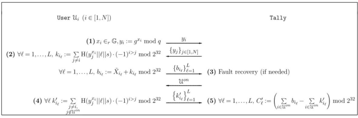
where the class is “female”. . . 64 4.1 Cryptographic layer of our private recommender system for

on-line streaming services. At setup (1), users compute their se-cret share and send their public key to the tally, who broad-casts them to the other users. During the encryption phase (2), each user computes the blinding factors, encrypts their Count-Min Sketch and sends it to the tally. In case not all

users have sent the data, the tally broadcasts Uon, the

sub-set ofusers that did (3). These compute new blinding factors and send them to the tally (4). Aggregate sketches are then recovered by the tally (5). . . 70 4.2 Execution time for increasing number of users (with 700

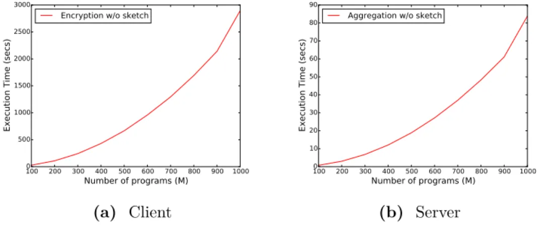
pro-grams). . . 74 4.3 Execution time for increasing number of programs (with 1,000

users). . . 75

4.4 Execution time for increasing number of programs (with 1,000

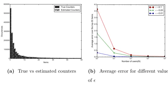
4.5 Visualizing the accuracy of the Count-Min Sketch for the most 50 frequent items (with 700 programs and sketch size 4,896). . . 78 4.6 Number of taxi locations over time. . . 79 4.7 Average error introduced by the Count-Min Sketch on the

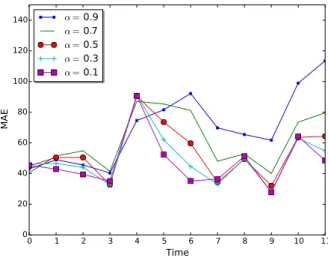
ag-gregate statistics for the top-100 locations. . . 80 4.8 Mean absolute error in the prediction for different values of

pre-diction algorithm’s parameter α. . . 81 4.9 Mean absolute error introduced by the Count-Min Sketch on

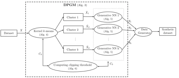
the prediction accuracy. . . 81 4.10 Count Sketch size versus estimation quality. . . 86 4.11 Quality versus differential privacy protection. . . 87 5.1 Overview of our differentially private generative model (DPGM)

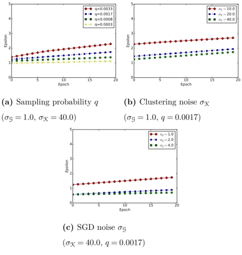
algorithm. . . 92 5.2 εvalue as a function of the number of SGD training epochs for

MNIST (δ= 10−5, T_K= 20) . . . 108 5.3 Clustering accuracy as a function of ε on MNIST (δ =

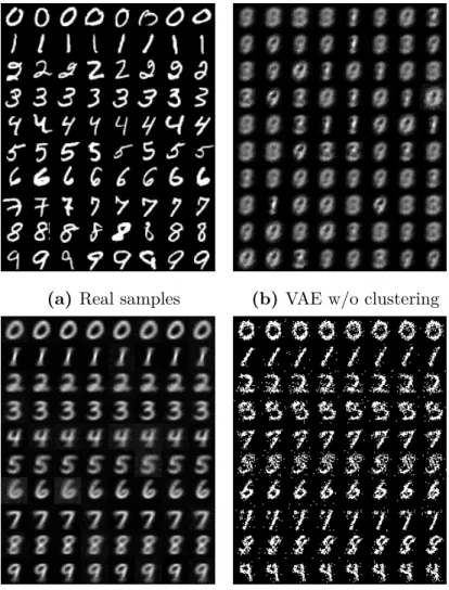
10−5, T_K= 20). . . 109 5.4 Real MNIST samples and samples generated from DPGM with

RBM and VAE after 20 epochs (ε= 1.74, T_K= 20). In (c) and (d), each row contains 8 samples generated from a cluster. . . . 110 5.5 Average relative error vs. ε for the CDR dataset (q = 2.2·

10−5, δ= 4.4·10−6) . . . 111 5.6 Average relative error vs. εfor the transit dataset (q= 10−4, δ=

10−6) . . . 112 5.7 Samples generated from a double layer VAE after 20 epochs.

Each row contains 8 samples generated from a cluster. . . 114 5.8 Average relative error with ε= 1.0 for the CDR and transit

datasets. . . 114 6.1 High-level Outline of the White-Box Attack. . . 118

6.2 White-Box Prediction Method: The attacker inputs data-points to the DiscriminatorD(1), extracts the output probabilities (2), and sorts them (3). . . 118 6.3 High-level overview of the (a) black-box attack with no auxiliary

knowledge, and (b)Discriminativeand (c)Generativeblack-box attack with limited auxiliary attacker knowledge. . . 119 6.4 Real samples. . . 122 6.5 Euclidean attack results for DCGAN target model trained on a

random 10% subset of CIFAR-10 and LFW. . . 125 6.6 Black-box attack results with 10% auxiliary attacker training set

knowledge used to train a DCGANshadow model for DCGAN target model trained on a random 10% subset of LFW. . . 125 6.7 Accuracy of white-box attack with different datasets and

train-ing sets. . . 126 6.8 Accuracy of black-box attack on different datasets and training

sets. . . 128 6.9 Membership inference accuracy using a discriminative model,

when the attacker has knowledge of (i) 20% of the test set, or (ii) 30% of both training and test sets. In (i), randomly guessing the training set corresponds to 14% accuracy, in (ii), to 12% accuracy. . . 130 6.10 Black-box attack results with 20% attacker training set

knowl-edge for DCGAN/DCGAN+VAE target models, trained on a random 10% subset of LFW, for different delays at which aux-iliary knowledge is introduced into the attacker model training. . 131 6.11 Black-box results when the attacker has (a) knowledge of 20% of

the training set or (b) 30% of the training set and test set. The training set is a random 10% subset of the LFW or CIFAR-10 dataset, and the target model is fixed as DCGAN. . . 132

6.12 Accuracy curves and samples at different stages of training on top ten classes from the LFW dataset, showing a clear correla-tion between higher accuracy and better sample quality. . . 133 6.13 Various samples from the real dataset, target model, and

black-box attack using the DCGAN target model on LFW, top ten classes. . . 133 6.14 Real and generated diabetic retinopathy dataset samples. . . 135 6.15 Accuracy curves of attacks against a DCGAN target model on

the Diabetic Retinopathy dataset. . . 136 6.16 Improvements over random guessing, in a black-box attack, as

we vary the size of the training set, and consider smaller subsets for training set predictions. . . 138 6.17 Improvement over random guessing for Weight Normalization

and Dropout defenses against white-box attacks on models trained over different number of classes with LFW. . . 141 6.18 Accuracy curve and samples for different privacy budgets on top

ten classes from the LFW dataset, showing a trade-off between samples quality and privacy guarantees. . . 142 7.1 Overview of inference attacks against collaborative learning. . . 145 7.2 Active property inference attack. . . 149 7.3 t-SNE projection of the features from different layers of the joint

model on LFW gender classification; 0 is female, 1 is male. The property (i.e., the blue points denoted by p-0 and p-1) is “race: black”, while the red points without the property are denoted by np-0 and np-1 . . . 156 7.4 AUC vs. the fraction of the batch that has the property on

FaceScrub and Yelp-author. . . 158 7.5 Detecting occurrence of a single-batch property. . . 158 7.6 Active property inference attack on FaceScrub. . . 160

7.7 Multi-party with synchronized SGD: attack AUC score vs. the number of participants. . . 161 7.8 Multi-party collaborative training with model averaging: box

plots show the distribution of the adversary’s scores in each trial. In the 8 trials on the left, one of the participants’ data has the property; in the 8 trials on the right, none of the honest participants have the data with the property. . . 162 7.9 Detecting when a participant whose local data has the property

of interest joins the training. K= 2 for rounds 0 to 250, K= 3 for rounds 250 to 500. . . 164 7.10 Uniqueness of user profiles with respect to the number of top

locations. . . 164 7.11 Attack performance with respect to the number of collaborative

List of Tables

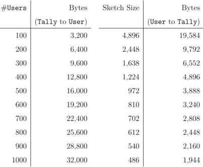
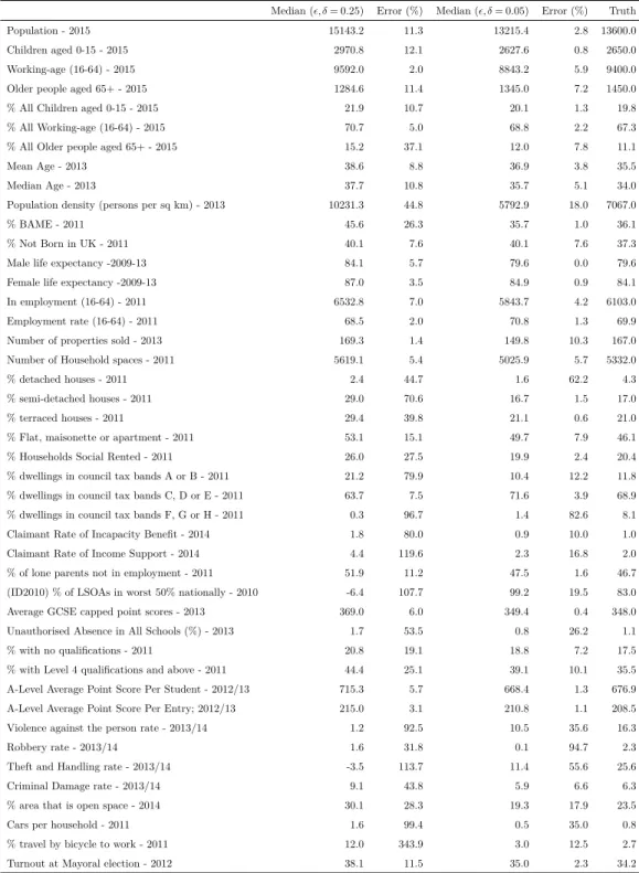
4.1 Bytes exchanged by user and tally for different #users and size of the Count-Min Sketch, considering 700 programs. . . 77 4.2 Median estimation with 22 ciphertexts (d = 2, w = 11, , δ =

0.25) and 165 ciphertexts (d= 3, w= 55, , δ= 0.05) on the London Atlas Dataset. . . 89 5.1 Notation and symbols used in this chapter. . . 93 5.2 The datasets used in our experiments: MNIST (images), CDR

(call detail records), and TRANSIT (transport records). . . 106 6.1 Accuracy of the best attacks on random 10% training set for

LFW and CIFAR-10, and for the diabetic retinopathy (DR) experiments. . . 136 7.1 Datasets and tasks used in our experiments. . . 151 7.2 Precision of membership inference (recall is 1). . . 153 7.3 AUC score of single-batch property inference on LFW. We also

report the Pearson correlation between the main task label and the property label. . . 155 7.4 Words with the largest positive coefficients in the property

clas-sifier for Yelp-health. . . 157 7.5 Inference attacks against the CSI Corpus for different fractions

of gradients shared during training. . . 165 7.6 Membership inference against the CSI Corpus and FourSquare

7.7 Inference of the top region (Antwerpen) on the CSI Corpus for different values of dropout probability. . . 167

List of Algorithms

1 Parameter server with synchronized SGD . . . 50 2 Federated learning with model averaging . . . 51 3 DPGM: Differentially Private Generative Model . . . 94 4 DPkmeans: Private kernel k-means with Random Fourier

Fea-tures . . . 96 5 Private Stochastic Gradient Descent . . . 100 6 DPNorm: Private Approximation of Average Norm . . . 101 7 Batch Property Classifier . . . 147

Introduction

With the widespread deployment of complex Internet-based services, large amounts of data, including sensitive information, are being constantly pub-lished, collected, and processed [45, 117]. This abundance of contextual in-formation makes it increasingly possible to extract value and knowledge from data. Examples include tracking GPS locations reported by mobile devices to generate live traffic maps (Google Traffic) and suggest more efficient routes [40]; analyzing social media content for disaster management [206], consumer confi-dence [161], and urban neighborhoods [181]; tracking disease inciconfi-dence through geographic analysis of web search queries on the use of specific key words over time [121]; generating artificially created multimedia content from real data, e.g., images [112] and videos [182]; enabling endpoint devices to jointly learn a common predictive model while keeping all the raw data in the device [143]. This dissertation focuses on the privacy challenges presented by two novel and demand-driven technological trends in data processing: (1)data collection, which is the process of gathering information from different input sources, and (2)machine learning (ML), which gives artificial intelligence systems the capability to acquire their own knowledge by extracting patterns from raw data [86].

First, the large-scale collection of user data raises serious privacy, confiden-tiality, and liability concerns, thus motivating the need for efficient and scalable techniques allowing providers to privately gather statistics. Rather than

re-leasing only specific aggregate statistics, such as certain counting queries or histograms, entities are often willing or compelled to publish their datasets, e.g., aiming to monetize it or allow third parties with the appropriate ex-pertise to analyze it. For instance, Call Detail Records (CDRs) collected by telecommunication companies are not only useful to capture interactions be-tween customers, but also to understand their behavior, e.g., for infectious disease spreading or migration patterns.1 As a result, telecommunications companies are often interested in releasing them in the form of “anonymized” datasets, which replace the original records in any data analytics without re-quiring any further interaction with the publisher.

However, as individuals usually have a unique combination of attribute values in these high-dimensional datasets, their exploitation and sharing are hindered by potential privacy breaches as well as implied monetary penalties. For instance, AOL released a detailed search logs dataset for research purposes, and Netflix released users’ ratings to allow an open competition for the best ML algorithm designed to predict user ratings for unseen movies. Personal identifiers such as names were removed from these datasets as a guarantee for the users in the datasets to remain anonymous. Nonetheless, Narayanan and Shmatikov [157] were later able to identify individual users by cross-referencing their data records, and both companies were sued for privacy breach.2,3

Second, over the past few years, ML has played a increasing role in data processing systems due to its capability of efficiently discovering valu-able knowledge and hidden information. Companies like Google, Microsoft, and Amazon provide customers with access to APIs that allow them to easily embed ML tasks into their applications. For instance, organizations provide Machine Learning as a Service (MLaaS) engines to outsource complex tasks, such as training classifiers, performing predictions, clustering, etc. They can also let other users query models trained on their data, possibly at a cost.

1_{See, e.g., http://www.flowminder.org}

2_{https://www.wired.com/2009/12/netflix-privacy-lawsuit/}

Among these techniques,generative modelsare an important emerging area in ML, as recent developments are paving the way for artificial generation of per-fectly plausible images and videos. They are used in a number of applications, e.g., compression [198], denoising [23], inpainting [221], super-resolution [125], semi-supervised learning [183], clustering [197], and deep neural networks pre-training [79] in cases where labeled data is expensive.

However, if malicious users can infer sensitive properties of data used to train these models, this leads to dangerous information leakage. More specifically, the ability of an adversary to ascertain the presence of a specific data point in a training dataset constitutes an immediate privacy threat if the dataset is sensitive per se. For instance, if a model was trained on the records of patients with a certain disease, learning that an individual’s record was part of the training data directly affects their privacy. On the one hand, users do not have much control over the kind of models and training parameters used by MLaaS platforms, and this might lead to overfitting (i.e., the model does not generalize well outside the data on which it was trained), thus making it easier for an attacker to perform inference attacks. On the other hand, this type of inference can also help enforce individual rights such as the “right to be forgotten”, demonstrate inappropriate uses of data (e.g., the use of health-care records to train ML models for unauthorized purposes [20]), and/or detect violations of data protection regulations such as the GDPR [81].

More recently, collaborative ML has emerged as an alternative to conven-tional MLaaS methodologies where all training data is pooled and the model trained on this joint pool. It allows two or more participants, each with his own training dataset, to work together to construct a joint model. More specif-ically, each participant trains a local model on his own data and periodically exchanges model parameters, updates to these parameters, or partially con-structed models with the other participants. Many architectures, systems, and protocols have been proposed for distributed, collaborative, and federated learning [63, 51, 215, 154, 129, 228]: with and without a central server, with

different ways of aggregating and averaging models, etc. Their typical goal is to improve the training speed and reduce overheads, but protecting the privacy of participants’ training data is an important motivation for several recent col-laborative learning systems [143, 190]. Because the training data never leaves the participants’ machines, collaborative learning may be considered as a good match for the scenarios where this data is sensitive (e.g., health-care records, private communications, personally identifiable information, etc.), and the par-ticipants want to construct a joint model without disclosing their datasets. Collaborative training, however, does disclose information via model updates that are indirectly based on the training data.

Together, these scenarios prompt a number of crucial challenges, including how to guarantee that the collected or published data are not misused; how to ensure that data processing does not lead to disclosure of sensitive information; and how to define privacy protection frameworks that allow usable and scalable services.

1.1

Research Questions

The broad goal of this dissertation is to tackle the following research problem:

Can we build and evaluate systems geared for privacy-friendly data process-ing, while enabling computational scenarios and applications where potentially sensitive data is needed to extract useful knowledge with strong privacy guar-antees?

Such goal entails addressing several open research questions, including: 1. Training ML models based on aggregate statistics gathered from many

data sources without disclosing fine-grained information about single sources and in an efficient manner.

2. Releasing synthetic datasets that resemble real datasets without incur-ring privacy breaches.

3. Evaluating if an adversary can infer information about the data used to train ML models.

1.2

Thesis Contributions

Overall, this dissertation investigates the design and evaluation of privacy-aware data processing mechanisms. The contributions of this dissertation in-clude:

1. We combine privacy-preserving aggregation with data structures sup-porting succinct data representation, namely,Count-Min Sketch [56] and Count Sketch [44]. Private aggregation is performed over the sketches, rather than the raw inputs. While an upper-bounded error in the ag-gregate is introduced, this allows us to reduce communication and com-putational complexity (for the cryptographic operations) fromlinear to logarithmic in the size of the inputs. We then use the resulting private statistics tools to instantiate protocols and build systems addressing real-world applications, where the error does not affect the overall quality of the computation. Specifically, we present and implement three protocols, (i) a privacy-preserving recommender system for on-line broadcasters, (ii) a private location prediction service, and (iii) a scheme for computing median statistics of Tor [65] hidden services in a private way.

2. We propose a novel approach, relying on generative neural networks, to model the data generating distribution of various kinds of data. It provides differential privacy [75] to each individual in the training data, thus, it can be used to effectively “anonymize” and share large high-dimensional datasets with any potentially adversarial third party. To this end, we present a Differentially Private Generative Model (DPGM), where data is first clustered, using the differentially private kernel k -means, and then each cluster is given to separate generative neural net-works which are trained only on their own cluster using differentially private gradient descent.

3. We study how generating synthetic samples through generative models may lead to information leakage, hence, to violating privacy of indi-viduals contributing their (sensitive) data to train these models. More specifically, given access to a generative model and an individual data record, we assess whether an attacker can tell if a specific record was used to train the model; this is also known as membership inference. Aiming to perform membership inference on generative ML models, we use Generative Adversarial Network (GAN) [87] models as a method to learn information about the target generative model, and thus create a local copy of the target model from which we can launch the attack. 4. We demonstrate that the training data used by participants in

collab-orative learning is vulnerable to a number of inference attacks. First, we show that an adversarial participant can infer the presence of exact data points of another participant’s training data (i.e., membership in-ference). We then propose passive and activeproperty inference attacks. These allow an adversarial participant in collaborative learning to infer properties of another participant’s training data that are not true of the class as a whole, or even independent of the features that characterize the classes of the joint model.

1.3

Thesis Structure

The remainder of this dissertation is organized as follows. Chapter 2 provides background about notions and main tools that are used throughout the dissertation. Then, Chapter 3 discusses relevant related work in the context of privacy-preserving data processing. Chapters 4 to 7 contain the technical contribution of this dissertation. In particular, Chapter 4 covers work done on privacy-preserving collection of statistics. Then, Chapter 5 presents the work done on the problem of automating the process of private data release. In Chapter 6, we tackle the problem of evaluating privacy leakage in generative ML models. Chapter 7 covers our work on the topic of inference attacks against

collaborative ML.

Finally, Chapter 8 concludes the dissertation with a discussion on our contributions, and offers some potential future directions.

1.4

Publications

The material in this dissertation has been submitted or published in con-ferences and journals, co-authored with several researchers. Specifically, work in Chapter 4 has been done in collaboration with George Danezis and Emil-iano De Cristofaro, and published in the proceedings of ISoc NDSS 2016 [147]. Chapter 5 presents the results of joint work with Gergely Acs, Claude Castel-luccia, and Emiliano De Cristofaro, and published in the proceedings of IEEE ICDM 2017 and in the IEEE TKDE journal [3]. Chapter 6 is the outcome of the collaborative work with Jamie Hayes, George Danezis, and Emiliano De Cristofaro, and currently under submission [94]. Finally, Conghzeng Song, Vi-taly Shmatikov, and Emiliano De Cristofaro have collaborated on the results presented in Chapter 7, and currently under submission [148].

1.5

Further Contributions

Besides the research included in this dissertation, we made further con-tributions with other researchers in the area of private network data process-ing. The associated research works have been published in the proceedings of the ACM CODASPY Workshop on SDN-NFV Security 2016 [149] and ACM SIGCOMM Workshop on Hot Topics in Middleboxes and Network Function Virtualization [13], in collaboration with Hassan Jameel Asghar, Mohamed Ali Kaafar, Cyril Soldani, Emiliano De Cristofaro, and Laurent Mathy.

Background

This chapter reviews concepts and tools in cryptography, succinct data structures, and machine learning that will be used throughout this dissertation.

2.1

Cryptography

We start by outlining some cryptographic primitives used in the rest of this dissertation.

2.1.1

Tools

Negligible function. A functionf(τ) is negligible in the security parameter τ if, for every polynomial p, it holds that f(τ)<_|p(1_t)|, for large enough t. Pairwise Independent Hash Functions. Let H be a family of random-lookinghash functions mapping values from a domain [D] to a range [R]. His pairwise independent if and only if ∀x6=y∈[D] and ∀a1, a2∈[R]:

Pr

h∈H[h(x) =a1∧h(y) =a2] =

1 R2.

Fully Homomorphic Encryption (FHE)A fully homomorphic encryption scheme (FHE) is a semantically secure cryptosystem that permits algebraic manipulations on plaintexts given their respective ciphertexts. More formally, a FHE scheme involves the following algorithms:

• Key generation: Given the security parameter k, generates public and private key pair (pk, sk).

• Encryption: Given plaintext m∈ {0,1}∗, outputs ciphertext c=E(m) encrypted under public keypk.

• Decryption: Given a ciphertext c, outputs the plaintextm=D(c) using the secret key sk.

• Homomorphic Addition (Add): Given two ciphertexts c1=E(m1), c2= E(m2), and the public key pk, produces a ciphertext c= Add(c1, c2) = c1+c2 such thatD(c) =m1+m2.

• Homomorphic Multiplication (Mult): Given two ciphertextsc1=E(m1), c2 =E(m2), and the public key pk, produces a ciphertext c as c= Mult(c1, c2) =c1·c2 such that D(c) =m1·m2.

A partial homomorphic encryption scheme only supports either addition or multiplication.

Homomorphic encryption schemes allow arbitrarily computations to be performed on encrypted data without decrypting it. For instance, homomor-phic encryption can be used to process encrypted DNA sequences in the cloud, or full text searching on encrypted data.

2.1.2

Assumptions

We now present some cryptographic assumptions used in the rest of this dissertation.

Computational Diffie Hellman Assumption (CDH). Let _G be a cyclic group of order q (|q|=τ, for security parameter τ), with generator g. We say that the Computational Diffie Hellman (CDH) problem is hard if, for any probabilistic polynomial-time algorithm ˆA and randomx, y drawn from _Zq:

PrhAˆ(_G, q, g, gx, gy) =gxyi is negligible in the security parameter τ.

Decisional Diffie Hellman Assumption (DDH). Let_Gbe a cyclic group of orderq(|q|=τ), with generatorg. We say that the Decisional Diffie Hellman

(DDH) problem is hard if, for any probabilistic polynomial-time algorithm ˆA0

and randomx, y, z drawn from _Zq:

Pr

ˆ

A

(

G

, q, g, g

, g

, g

) = 1

−

Pr

A

ˆ

(

G

, q, g, g

, g

, g

) = 1

is negligible in the security parameter τ.

These assumptions are based on problems involving discrete logarithms in cyclic groups. They are commonly used as the basis to prove the security of many cryptographic protocols, e.g., the ElGamal cryptosystem [78]. The DDH and CDH assumptions are related to each other. If it were possible to efficiently compute gxy from (gx, gy), then one could easily distinguish the two probability distributions in DDH. It is believed that DDH is a stronger assumption than CDH. DDH and CDH are variants of the more general Diffie Hellman problem (DHP) in which, given g, gx and gy, the problem is to find the value of gxy. The main motivation for this problem is that many security systems rely on one-way functions, i.e., operations that are fast to compute, but hard to reverse. In cryptography, one-way functions enable encrypting a message, while making it difficult to decrypt the same message without knowing some private information. If it were possible to efficiently solve DHP, then security systems that rely on DHP would be easily broken.

2.1.3

Differential Privacy (DP)

Differential privacy can be motivated by the impossibility result, for a statistical database, to achieve the privacy goal of preventing disclosure about any individual against adversaries with arbitrary auxiliary while still providing any useful information. We can further consider the following example taken from [69]:

Given a statistical database that provides the average height for pop-ulation subgroups, and the auxiliary information “Terry Gross is two inches shorter than the average Lithuanian woman”. An adversary with this auxiliary information and access to the database is able to recover Terry Gross’ height, whereas an adversary with only auxiliary information learns much less about

Terry Gross’ height. However, Terry Gross is not required to be part of the statistical database in order for this privacy breach to happen. Therefore, dif-ferential privacy notion aims tominimize the increased risk that an individual incurs by joining – or leaving – the database [69].

More concretely, differential privacy allows a party to privately release a dataset: using perturbation mechanisms, a function of an input dataset is modified, so that any information which can discriminate a record from the rest of the dataset is bounded [75]. Hence, any information that can be learned from the database with a record can also be learned from the one without this record. Consequently, for a record owner, it means that any privacy breach will not be due to participating in the database.

More formally, ε-differential privacy is defined as follows:

Definition 1(ε-Differential Privacy [75]). A privacy mechanismAguarantees ε-differential privacy if for any databaseX∈XandX0∈Xdiffering on at most one record, and for any possible output O∈Range(A),

e−ε×P r[A(X0) =O]≤P r[A(X) =O]≤eε×P r[A(X0) =O] where the probability is taken over the randomness of A.

Intuitively, this guarantees that an adversary, provided with the output of

A, can draw almost the same conclusions about any individual no matter if this individual is included in the input ofAor not [75]. The following definition of privacy loss can then be formally derived.

Definition 2 (Privacy loss). Let A be a privacy mechanism which assigns a value O ∈ Range(A) to a dataset X ∈ X. The privacy loss of A with datasets X ∈X and X0 ∈X at output O ∈Range(A) is a random variable

P(A, X, X0, O) = log_Pr[Pr[_AA₍(_XX0)=₎₌O_O]_] where the probability is taken on the

random-ness of A.

A relaxation of DP is probabilistic-DP, or (, δ)-DP, where privacy breaches may occur with very small probability.

Definition 3 ((, δ)-Differential Privacy [75]). A privacy mechanism A guar-antees(ε, δ)-differential privacy if for any databaseX∈XandX0∈X, differing on at most one record, and for any possible output S⊆Range(A),

P r[A(X)∈S]≤eε×P r[A(X0)∈S] +δ or, equivalently,

Pr

O∼A(X)[P(A, X, X

0_{, O)> ε]≤δ.}

This definition guarantees that every output of algorithm A is almost equally likely (up to ε) on datasets differing in a single record except with probability at most δ, preferably smaller than 1/|X|. Probabilistic-DP pro-vides higher utilities in practice thanε-DP (Definition 1) at the cost of weaker privacy guarantees.

A fundamental concept in DP is theglobal sensitivity of a function [75]. Definition 4 (Global Lp-sensitivity). For any function f :X→Rd, the Lp

-sensitivity of f is ∆pf = maxX,X0||f(X)−f(X0)||_p, for all X, X0 differing in

at most one record, where || · ||p denotes the Lp-norm.

There are a few ways to achieve DP, including the Laplace mechanism and the Gaussian mechanism. The Laplace mechanism (LPM) consists of adding noise sampled from the Laplace distribution to the true output of a function. Definition 5(Laplace mechanism (LPM) [75]). For any function f:X→_Rd_,

LPM is defined as

LP(X) =f(X) + [ˆY1(ˆs), . . . ,Yˆd(ˆs)]

whereYˆi(ˆs)are i.i.d Laplace random variables with scale parametersˆ= ∆1f /ε, and ∆1f is the L1-sensitivity off.

It can be proved that the above definition of LPM achieves ε-DP [75]. Instead, the Gaussian Mechanism (GM) consists of adding gaussian noise to the true output of a function.

Definition 6 (Gaussian Mechanism (GM) [75]). For any function f:X→_Rd_,

GM is defined as

G(X) =f(X) + [N1(0,∆2f·σ), . . . ,Nd(0,∆2f·σ)]

where Ni(0,∆2f·σ) are i.i.d. normal random variables with zero mean and variance (∆2f·σ)2, and ∆2f is the L2-sensitivity of f.

The above definition of GM is (ε, δ)-DP if σ ≥ ∆2f /ε for c2 > 2 ln(1.25)/δ [75].

The output of any randomized algorithm remains differentially private if all inputs are already differentially private. This is often referred to as the post-processing property of DP. Further, DP maintains composition.

Theorem 1 (Composition property of DP [145]). Let Ai each provide εi

-differential privacy. It holds:

1. A sequence of Ai(X) over the dataset X provides Piεi-differential

pri-vacy.

2. A sequence ofAi(Xi)over a set of disjoint1 datasetsXiprovidesmax(εi

)-differential privacy.

In the case of probabilistic-DP, if each ofA1, . . . ,Akis (ε, δ)-DP, then their

k-fold adaptive composition2 is (kε, kδ)-DP. However, a tighter upper bound can be derived on the privacy loss of the composite using a generic Chernoff bound. In particular, it follows from Markov’s inequality that

Pr[P(A, X, X0, O)≥ε]≤_E[exp(λP(A, X, X0, O))]/exp(λε)

for any outputO∈Range(A) and λ >0. This implies thatAis (ε, δ)-DP with δ= min_λexp(β_A(λ)−λε), whereβ_A(λ) = max_X,X0log_EO∼A(X)[exp(λP(A, X, X0, O))]

is the log of the moment generating function of the privacy loss.

1_{Two datasets are disjoint if they have no common records.} 2_{The output of A}

i−1 is used as input to Ai, i.e., their executions are not necessarily independent except their coin tosses.

This result is referred to as the moments accountant method, which we formally define as follows:

Theorem 2 (Moments accountant (Abadi et al. [1])). Let β_Ai(λ) be max

X,X0logEO∼A(X)[exp(λP(A, X, X 0_{, O))]}

and A_1:k the k-fold adaptive composition of A1,A2, . . . ,Ak. It holds:

1. β_A1:k(λ)≤Pk

i=1βAi(λ)

2. A_1:k is (ε,min_λexp(Pk

i=1βAi(λ)−λε))-differentially private

where A1,A2, . . . ,Ak use independent coin tosses.

Moreover, if an increase in theδterm is tolerated, the privacy parameterε degrades proportionally to√k, and the composite is (ε·O(qklog(1/δ0)), kδ+ δ0)-differentially private for all k <1/ε2 and δ0>0. This result is known as the advanced composition property of differential privacy [71].

Finally, we introduce the following useful Lemma.

Lemma 1. Let Gbe the Gaussian Mechanism. It holds: β_G(λ) = (λ2+λ)/4σ2

Proof. Letf:X→_R be a scalar function, f(X) =f(X0) + ∆1f, where ∆1f= ∆2f, and O=f(X) +x, wherex∼N(0, σ). Let ˆσ= ∆1f·σ Then, it holds:

P(A, X, X0, O) = ln Pr[G(X) =O] Pr[G(X0_{) =O]} ! = = ln Pr[f(X) +N(0,σ) =ˆ O] Pr[f(X0) +N(0,σ) =ˆ O] ! = ln exp(−x 2_/2ˆσ2₎ exp(−(x+ ∆1f)2/2ˆσ2) ! = = ln exp(−x 2_/2ˆσ2₎ exp(−(x+ ∆1f)2/2ˆσ2) ! = ∆1f ˆ σ · x ˆ σ ! +1 2 ∆1f ˆ σ !2

Sincexis drawn fromN(0,σ),ˆ P(A, X, X0, O) follows a normal distribution with mean (∆1f)2/2ˆσ2 and standard deviation ∆1f /σ, whose moment generatingˆ function is exp(λ2+λ)(∆1f)2/4ˆσ2

. The claim follows from the definition of β and ˆσ. For the high-dimensional case when f :X→_Rd (d >1), the proof is similar to that of Theorem A.1 in [75].

Figure 2.1: Update procedure for the Count-Min Sketch.

Given β_G(λ), the exact privacy cost ε (or δ) of the k-fold adaptive com-position of Gis computed based on Theorem 2.

2.2

Succinct Data Structures

This section introduces some succinct data structures, namely Count-Min Sketch and Count Sketch, for efficient query operations. These “sketching” data structures use minimal space to allow estimating the most frequent items in a large set of data. They are used in a number of applications, e.g., tracking Twitter’s most popular tweets, or counting the most visited pages of a website. Count-Min Sketch [56] is a data structure that can be used to provide a succinct sublinear-space representation of multi-sets. An interesting prop-erty is that they enable aggregation of the multi-sets represented by two or more sketches using a linear operation on the sketches themselves. Prior uses of Count-Min Sketch include summarizing large amounts of frequency data for sensing, networking, natural language processing, and database applica-tions [62].

Definition 7(Count-Min Sketch). A Count-Min Sketch with parameters(, δ) is a two-dimensional array (table) X, with width˜ w and depth d. Given pa-rameters (, δ), set d=dlnT /δe and w=de/e, where T is the number of items to be counted. Each entry of the table is initialized to zero. Then, d hash functions hj :{0,1}∗→ {0,1}w, are chosen uniformly at random from a

pairwise-independent family H.

Update Procedure. To update itemiby a quantityci,ciis added to one element

in each row, where the element in row j is determined by the hash function hj. The update is denoted as (i, ci). More precisely, to update the count for

item i toci∈N, for each row j of ˜X, set:

˜

X[j, hj(i)]←X[j, h˜ j(i)] +ci

This procedure is illustrated in Figure 2.1.

Estimation Procedure. To estimate the count ˆci for item i, we take the

mini-mum of the estimates of ci from every row of ˜X:

ˆ

ci←min j

˜

X[j, hj(i)]

Error Upper Bound. Given estimate ˆci, it holds:

1. ci≤cˆi

2. ˆci≤ci+PTj=1|cj| with probability 1−δ.

(whereci is the true counter).

Count Sketch [44] is a data structure which provides an estimate for an item’s frequency in a stream. Count Sketch has the same update procedure as Count-Min Sketch, but differs in the estimation. Specifically, given the table

˜

X built on the stream, the row estimate ofci (which is the counter of item i)

for rowj is computed based on two buckets: ˜X[i, hj(i)] and ˜X[i, h0j(i)], where

h0_j(i) is defined as:

h0_j(i) :=       

hj(i)−1 if hj(i) mod 2 = 0

hj(i) + 1 if hj(i) mod 2 = 1

The estimate ofci for row j is then

˜

X[j, hj(i)]−X[j, h˜ 0j(i)]

To estimate the count ˆci for itemi, we take the sum of the estimates ofcifrom

every row of X: ˆ ci←sum j ˜ X[j, hj(i)]−X[j, h˜ 0j(i)]

Both Count-Min and Count Sketch are linear: the element-wise sum of the sketches representing two multi-sets yields the sketch of their union.

Note that, although we use (, δ) to denote parameters for both Count(-Min) Sketch and differential privacy (see Section 2.1.3), it is clear from the context which one it relates to.

2.3

Machine Learning

In this section, we review machine learning concepts used throughout the dissertation.

2.3.1

Recommender systems

Recommender systems are used to predict the utility of a certain item for a particular user, based on their previous ratings as well as those of other “similar” users [180]. Consider a set of N users and a list of M items: for each user, a rating can be associated to each item, based, e.g., on the user’s explicit opinion about the item (e.g., 1 to 5 stars) or by implicitly deriving it from purchase records or browser history.

Machine learning can be used to predict the expected rating of an unrated item for a given user. TheK-Nearest Neighbor (KNN) classification algorithm finds the top-K nearest neighbors for a given item, so that ratings associated with these are combined to predict unknown ratings. A variant of KNN is called ItemKNN [185]. The algorithm is trained using an item-to-item simi-larity matrix (correlation matrix), where each element expresses the simisimi-larity between a pair of items, and the Cosine Similarity is computed between vectors of items (e.g., user ratings for each item).

If ratings are binary values (e.g., viewed/not viewed), the Cosine Similar-ity between items a and b is:

{Sim}_ab=√Cab Ca·Cb

(2.1) where C_ab, Ca, and Cb denote, respectively, the number of people who rated

neighbors for each item as the items with the highest correlation values. The final model then consists of the identity of the nearest neighbors and their correlation values (or weights) which are used in the prediction process, i.e., the items that should be recommended.

Note that, with ItemKNN, given the item-to-item matrix, each user could independently compare their ratings with the nearest neighbors of each item in the model. Upon finding a match, the weight is added to the prediction score for that item. The items are then ranked by their prediction scores and the top K are taken as recommendations. Predicting user ratings or interests in general has many applications especially in e-commerce systems (e.g. Amazon Web store).

2.3.2

Time-series data prediction

Time-series data prediction can be performed, among others, using Ex-ponential Weighted Moving Average (EWMA) models [192]. EWMA can pre-dict future values based on past values weighted with exponentially decreasing weights toward older values. Given a signal over time r(t), we indicate with ˜

r(t+ 1) the predicted value of r(t+ 1) given the past observations, r(t0), at time t0≤t. Predicted signal ˜r(t+ 1) is estimated as:

˜ r(t+ 1) = t X t0₌₁ α(1−α)t−t0r(t0)

where α ∈(0,1) is the smoothing coefficient, and t0 = 1, . . . , t indicates the training window, i.e., 1 corresponds to the oldest observation while t is the most recent one.

2.3.3

Kernel k-means with random features

Clustering is the task of grouping a set of objects in such a way that objects in the same group, or cluster, are more similar to each other than to those in other groups. k-means is one of the most popular clustering algorithms. Given a set of samples X ={x1, x2, . . . , xN}, k-means linearly separates X

Pk i=1

P

x∈Ci||x−ci||

2

2, where ci=Px∈Cix/|Ci| is the centroid of cluster Ci.

Although this problem is NP-hard, there are efficient heuristic algorithms (such as Lloyd’s algorithm) which iteratively refines clustering and converge quickly to a local optimum. However, k-means can provide very inaccurate clustering of linearly non-separable data, which are very common in practice.

To overcome this shortcoming, kernel k-means [187] first maps samples from input space to a higher dimensional feature space through a non-linear transformation Φ, then applies standardk-means on{Φ(x1),Φ(x2), . . . ,Φ(xN)}.

Hence, kernel k-means provides linear separators of clusters in feature space which correspond to non-linear separators in input space. Kernel k-means iteratively computes||Φ(x)−c0_i||2

2 for each sample x to decide which cluster a sample belongs to, where c0_i=P

x∈CiΦ(x)/|Ci|. To do so, the inner product

hΦ(x),Φ(y)i must be known for all x, y ∈X. Since Φ(·) is hard to explicitly compute due to its large, often infinite dimension, the kernel trick is applied; hΦ(x),Φ(y)i=κ(x, y), where κ is an easily computable kernel function. Still, this approach requires evaluating κ for all pairs of samples and store the results, which is not scalable for large datasets.

To make kernel k-means scalable, the kernel function can be approxi-mated with low-dimensional explicit feature maps. In particular, the samples are first mapped to a low-dimensional Euclidean inner product space using an explicit random feature map z:_Rm→_Rd _{so that hΦ(x),Φ(y)i ≈ hz(x), z(y)i.}

Then, standard k-means is applied on the low-dimensional mapped samples {z(x1), z(x2), . . . , z(xN)}inRd to approximate the result of the kernelk-means

with implicit feature map Φ and kernel κ. Although the approximation error decreases as d increases, quite accurate approximations can be obtained even for d < m. Explicit nonlinear feature maps have already been proposed for shift-invariant kernels (e.g., generalized RBF kernels) [207] as well as polyno-mial kernels [170] among others.

2.3.4

Neural networks

In recent years, a family of machine learning models known as deep neural networks (ordeep learning) has become very popular for many machine learn-ing tasks, especially related to computer vision and image recognition [186, 123]. Deep learning models are made of layers of non-linear mappings from input to intermediate hidden states and, finally, to output. Each connection between layers has a floating-point weight matrix as parameters. These weights are updated during training. The topology of the connections between layers is task-dependent and important for the ultimate accuracy of the model. To find the optimal set of parameters that fits the training data, the training al-gorithm optimizes the objective (loss) function L, which penalizes the model when it outputs a wrong label on a data point.

There are many methods to optimize the objective function. Stochastic gradient descent (SGD) and its variants (e.g., Adam optimizer [116]) are com-monly used to train artificial neural networks. SGD is an iterative method where at each step the optimizer receives a small batch of the training data and updates the model parametersθ according to the direction of the negative gradient of the objective function with respect to θ and scaled by the learn-ing rate η∈_R+_{. Training finishes when the model has converged to a local} minimum, where the gradient is close to zero.

Machine learning models include discriminative and generative ones. Given a supervised learning task, and given the features of a data-pointx∈X and the corresponding label y∈Y, discriminative models attempt to predict y on futurex by learning a discriminative functionf from (x, y); the function takes in input x and outputs the most likely label y. Discriminative models are not able to “explain” how the data-points might have been generated. By contrast, generative models describe how data is generated by learning the joint probability distribution of p(X, Y), which gives a score to the configu-ration determined together by pairs (x, y). Generative models based on deep neural networks, such as Generative Adversarial Networks (GAN) [87] and

Variational Auto-encoders (VAE) [115] are considered as the state-of-the-art for producing samples of realistic images [111].

We now briefly describe three generative neural networks models used in this dissertation in Chapters 5 and 6.

Restricted Boltzmann Machines (RBM). A Restricted Boltzmann Ma-chine (RBM) is a bipartite undirected graphical model composed of m visible and n invisible (or latent) binary random variables denoted by, respectively, v= (v1, v2, . . . , vm) and h= (h1, h2, . . . , hn). Visible variables represent the

at-tributes of x and their values are composed of records from X. Hidden vari-ables capture the dependencies between different visible varivari-ables. As the above model is a Markov random field with strictly positive joint probability distribution ˜p over the model variables, ˜p can be represented as a Boltzmann distribution defined as:

˜

p(v, h) = 1 Ze

−E(v,h) _(2.2)

whereZ=P

v,he−E(v,h) is the partition function, E(v, h) the energy function,

i.e., E(v, h) =−Pn i=1

Pm

j=1·Wij·hi·vj−Pmj=1bjvj−Pni=1cihi, with Wij being

real valued weights describing the inter-dependency between vj and hi, and

bj, ci real valued bias terms associated with the jth visible and ith hidden

units, respectively. Using matrix notation, E(v, h) =−v·W·h−b·v−c·h, where W ={Wi,j}, c={ci}, and b={bj}. The goal is to approximate the

true data generating distribution with the Boltzmann distribution ˜p, given in Eq. (2.2). To this end, we train the RBM model on dataset X to compute parameters (W, b, c).

There are a few algorithms to train RBMs, that approximate or relate to gradient descent on the log-loss of the data. If θ= (W, b, c), then we want to minimize the loss function L(X;θ) =−Q

x∈Xp(x|θ) given dataset˜ X, where

x∈ {0,1}m is a record from X and ˜p is the Boltzmann distribution defined in Eq. (2.2). The model parameters are updated until the log-loss converges using Persistent Contrastive Divergence [199].

Variational Autoencoder (VAE).A variational autoencoder [115] consists of two neural networks (an encoder and a decoder), and a loss function. The encoder compresses data into a latent space z while the decoder reconstructs the data given the hidden representation. Let x be a random vector of m observed variables, which are either discrete or continuous. Letz be a random vector of n latent continuous variables. The probability distribution between x and z assumes the form p_θ(x, z) =p_θ(z)p_θ(x|z), where θ indicates that p is parametrized by θ. Also, let qφ(z |x) be a recognition model whose goal

is to approximate the true and intractable posterior distribution p_θ(z |x). We can then define a lower-bound on the log-loss of x as follows: L(x;θ) = D_KL(q_φ(z|x)||p_θ(z))−_Eqφ(z|x)[logp_θ(x|z)]. The first term pushes q_φ(z|x) to be similar topθ(z) ensuring that, while training, VAE learns a decoder that,

at generation time, will be able to invert samples from the prior distribution such they look just like the training data. The second term can be seen as a form of reconstruction cost, and needs to be approximated by sampling from qφ(z|x).

In VAEs, we propagate the gradient signal through the sampling process and throughqφ(z|x) using thereparametrization trick. This is done by making

z be a deterministic function of φ and some noise ξ, i.e., z =f(φ, ξ). For instance, sampling from a normal distribution can be done like z =µ+σξ, where ξ∼N(0, I). The reparametrization trick can be viewed as an efficient way of adapting qφ(z |x) to help improve the reconstruction. We train the

variational autoencoder using stochastic gradient descent to optimize the loss with respect to the parameters of the encoder and decoder θ and φ.

Generative Adversarial Network (GAN).GANs [87] are neural networks trained in an adversarial manner to generate data mimicking some distribution. The main intuition is to have two competing neural network models. One model, the generator, takes noise as input and generates samples. The other model, the discriminator, receives samples from both the generator and the training data, and has to be able to distinguish between the two sources.

Figure 2.2: Generative Adversarial Network (GAN).

The two networks play a continuous game where the generator is learning to produce more and more realistic samples, and the discriminator is learning to get better and better at distinguishing generated data from real data, as depicted in Figure 2.2.

More formally, to learn the generator’s output distribution over data-points x, we define a prior on input noise variables pz(z), then represent a

mapping to data space asG(z;θg), whereGis a generative deep neural network

with parameters θg. We also define a discriminator D(x;θd) that outputs

D(x)∈[0,1], representing the probability thatx was taken from the training set rather than from the generatorG. Dis trained to maximize the probability of assigning the correct label to both real training examples and fake samples from G. We simultaneously train G to minimize log(1−D(G(z))). The final optimization problem solved by the two networksDandGfollows a two-player minimax game as:

min

G maxD Ex∼pdata(x)[logD(x)] +Ez∼pz(z)[log(1−D(G(z)))]

First, gradients ofD are computed to discriminate fake samples from training data, thenGis updated to generate samples that are more likely to be classified as data. After several steps of training, ifG and D have enough capacity and a Nash equilibrium is achieved, they will reach a point at which both cannot improve [87].

Larsen et al. [122] combine VAEs and GANs into an unsupervised gener-ative model that simultaneously learns to encode and generate new samples, which contain more details, sampled from the training data-points.

Figure 2.3: Collaborative Learning.

Recently, Lucic et al. [135] show that, despite a large number of proposed changes to the original GAN model [141, 25, 118, 12, 90], it is still difficult to assess if one performs better than another. They also show that the original GAN performs equally well against other state-of-the-art GANs, concluding that any improvements are due to computational budgets and hyper-parameter tuning, rather than scientific breakthroughs.

2.3.5

Collaborative learning

Training a deep neural network on a large dataset can take long time. A common approach to scale deep learning [51, 63] is to partition the train-ing dataset, concurrently train separate models on each subset, and exchange parameters via a parameter server which stores the global set of all model parameters (see Figure 2.3). During training, each local model pulls the pa-rameters from this server, calculates the updates based on its current batch of training data, then pushes these updates back to the server, which updates the global parameters.

Collaborative learning may involve participants who want to hide their training data from each other. We review two architectures for privacy-preserving collaborative learning based on, respectively, [190] and [143]. Parameter server with synchronized gradient updates. We con-sider collaborative learning with synchronized gradient updates, as proposed

Algorithm 1: Parameter server with synchronized SGD 1 Server executes:

2 Initialize θ₀ 3 for t= 1 to T do 4 for each client k do

5 g_tk←ClientUpdate(θ_t−1)

6 θ_t←θ_t−1−ηP_kg_tk .synchronized gradient updates 7

8 ClientUpdate(θ):

9 Select a batch B from client’s data 10 return local gradients ∇L(B;θ)

in [190]: see Algorithm 1. In each iteration of training, the participants down-load the global model from the parameter server. Each participant then locally computes gradient updates based on one batch of his training data and sends the updates to the server. The server waits for the gradient updates from all participants and then applies the aggregated updates to the global model using stochastic gradient descent (SGD).

Federated learning with model averaging. We also consider the federated learning framework proposed in [143]: see Algorithm 2. The parameter C controls the fraction of the K participants that update the model in round t. In each round, the k-th participant locally takes several steps of SGD on the current model using his entire local training dataset of size nk (i.e., the globally visible updates are based not on batches but on participants’ entire datasets). In the algorithm description, n corresponds to the total size of the training data, i.e., the sum of all nk. Each participant submits the resulting model to the server, which computes a weighted average of the models. The server evaluates the resulting joint model on a held-out dataset and stops training when performance stops improving.

Algorithm 2: Federated learning with model averaging 1 Server executes:

2 Initialize θ₀

3 m←max(C·K,1) 4 for t= 1 to T do

5 S_t←(random set of m clients) 6 for each client k∈S_t do 7 θk_t ←ClientUpdate(θ_t−1) 8 θ_t←P_kn

k

nθ k

t . averaging local models

9

10 ClientUpdate(θ):

11 for each local iteration do

12 for each batch B in client’s split do 13 θ←θ−η∇L(B;θ)

14 return local modelθ

depends on the specific learning task and the hyper-parameters (e.g., number of participants, batch size, etc.).

Related Work

In this chapter, we discuss prior work on privacy-friendly data processing, focusing on private statistics and privacy in machine learning.

3.1

Private Statistics

This section reviews prior work on privacy-preserving techniques applied to data aggregation, as well as efficient data structures for succinct represen-tation.

3.1.1

Privacy-preserving aggregation

Private aggregation schemes like ANONIZE [97] and PrivStats [173] rely on anonymizing networks, such as Tor [65], to protect privacy against net-work adversaries. Unfortunately, Tor-based schemes are vulnerable to traffic-analysis attacks [155]. Dining Cryptographers anonymizing networks, or DC-nets, are instead used in [58, 60, 61]. However, DC-nets require expensive operations at the servers side.

Other schemes [120, 39, 107, 59] provide strong privacy guarantees via secret-sharing based methods. In particular, Kursawe et al. [120] introduce a few cryptographic constructions to aggregate energy consumptions in the context of smart metering, relying on Diffie-Hellman, bilinear maps, and a “low overhead” protocol where meters’ encryption keys sum up to zero. Our schemes for the private recommender system and location prediction – pre-sented in Chapter 4 – rely on a protocol inspired by [120]’s “low overhead”

protocol, but perform private aggregation using succinct data representation rather than the raw inputs. Using C