San Jose State University
SJSU ScholarWorks
Master's Projects Master's Theses and Graduate Research
Spring 5-20-2019
Speaker Recognition Using Machine Learning
Techniques
Abhishek Manoj Sharma San Jose State University
Follow this and additional works at:https://scholarworks.sjsu.edu/etd_projects
Part of theArtificial Intelligence and Robotics Commons
This Master's Project is brought to you for free and open access by the Master's Theses and Graduate Research at SJSU ScholarWorks. It has been accepted for inclusion in Master's Projects by an authorized administrator of SJSU ScholarWorks. For more information, please contact
Recommended Citation
Sharma, Abhishek Manoj, "Speaker Recognition Using Machine Learning Techniques" (2019).Master's Projects. 685. DOI: https://doi.org/10.31979/etd.fhhr-49pm
1
Speaker Recognition Using Machine Learning Techniques
A Thesis
Presented to
The Faculty of the Department of Computer Science San José State University
In Partial Fulfillment
of the Requirements for the Degree Master of Science
by
Abhishek Manoj Sharma May 2019
2
The Designated Thesis Committee Approves the Thesis Titled
Speaker Recognition Using Machine Learning Techniques
by
Abhishek Manoj Sharma
APPROVED FOR THE DEPARTMENT OF COMPUTER SCIENCE
SAN JOSÉ STATE UNIVERSITY
May 2019
Dr. Robert Chun Department of Computer Science Dr. Thomas Austin Department of Computer Science Mr. Nishad Desai Oracle Corporation
3
ABSTRACT
Speaker recognition is a technique of identifying the person talking to a machine using the voice features and acoustics. It has multiple applications ranging in the fields of Human Computer Interaction (HCI), biometrics, security, and Internet of Things (IoT). With the advancements in technology, hardware is getting powerful and software is becoming smarter. Subsequently, the utilization of devices to interact effectively with humans and performing complex calculations is also increasing. This is where speaker recognition is important as it facilitates a seamless communication between humans and computers. Additionally, the field of security has seen a rise in biometrics. At present, multiple biometric techniques co-exist with each other, for instance, iris, fingerprint, voice, facial, and more. Voice is one metric which apart from being natural to the users, provides comparable and sometimes even higher levels of security when compared to some traditional biometric approaches. Hence, it is a widely accepted form of biometric technique and is constantly being studied by scientists for further improvements. This study aims to evaluate different pre-processing, feature extraction, and machine learning techniques on audios recorded in unconstrained and natural environments to determine which combination of these works well for speaker recognition and classification. Thus, the report presents several methods of audio pre-processing like trimming, split and merge, noise reduction, and vocal enhancements to enhance the audios obtained from real-world situations. Additionally, a text-independent approach is used in this research which makes the model flexible to multiple languages. Mel Frequency Cepstral Coefficients (MFCC) are extracted for each audio, along with their differentials and accelerations to evaluate machine learning classification techniques such as kNN, Support Vector Machines, and Random Forest Classifiers. Lastly, the approaches are evaluated against existing research to study which techniques performs well on these sets of audio recordings.
Key terms: Speaker recognition, human computer interaction, biometrics, internet of things, mel frequency cepstral coefficients
4
ACKNOWLEDGMENTS
I would like to thank my advisor, Dr. Robert Chun for his continuous support and guidance. His experience has greatly helped me during my research and I am truly grateful for getting an opportunity to work with him.
I would also like to thank my committee members, Dr. Thomas Austin and Mr. Nishad Desai for their valuable time, support, guidance, and feedback.
I also extend my gratitude to the Department of Computer Science and all the faculty members I have interacted with during my academic program. Thanks for enriching my knowledge and making it a memorable experience.
Lastly, I would like to thank my parents, relatives, and friends for always supporting me and believing in me.
5 TABLE OF CONTENTS 1. Introduction ... 7 1.1. Importance ... 8 1.2. Motivation ... 9 2. Existing Work... 10
2.1. Feature Extraction Techniques for Speaker Recognition ... 11
2.2. Vectorization Techniques in Speaker Recognition ... 12
2.3. Genetic Algorithms in Speaker Recognition... 14
2.4. SVM and Naïve Bayes Machine Learning Techniques for Speaker Recognition ... 15
2.5. Neural Network in Speaker Recognition ... 18
3. Feature Extraction ... 21
3.1. Audio Framing ... 22
3.2. Mel Frequency Cepstral Coefficients (MFCC) ... 23
3.3 MFCC Delta: Differentials... 24
3.4. MFCC Delta-Delta: Accelerations ... 25
3.5. Edge Trimming ... 25
4. Machine Learning Classifiers ... 27
4.1. Support Vector Machine (SVM) ... 27
4.2. Random Forest Classifier ... 30
4.3. k Nearest Neighbors ... 32
5. Dataset ... 33
5.1 VoxCeleb Dataset ... 33
5.2. Dataset Diversity ... 34
6. Tools and Libraries ... 36
6.1. LibROSA ... 36
6.2. python_speech_features ... 36
6.3. Scikit-learn ... 36
6.4. Other Python libraries: ... 36
7. Implementation ... 37
7.1. Ambient Noise Reduction ... 37
6
7.3. Audio Trimming ... 39
7.4. Audio Splitting ... 39
7.5. Feature Extraction ... 41
7.6. Machine Learning Classification ... 43
8. Evaluation Metrics ... 44 8.1. Confusion Matrix ... 44 8.2. Classification Accuracy ... 45 8.3. Precision ... 45 8.4. Recall ... 45 8.5. F-1 Score ... 46 9. Experiments ... 47 Experiment 1: SVM + MFCC Coefficients ... 47
Experiment 2: SVM + MFCC Delta Coefficients ... 49
Experiment 3: SVM + MFCC Delta Delta Coefficients ... 51
Experiment 4: Random Forest + MFCC Coefficients ... 53
Experiment 5: Random Forest + MFCC Delta Coefficients ... 54
Experiment 6: Random Forest + MFCC Delta Delta Coefficients ... 55
Experiment 7: kNN + MFCC Coefficients ... 56
Experiment 8: kNN + MFCC Delta Coefficients ... 58
Experiment 9: kNN + MFCC Delta Delta Coefficients ... 59
10. Results ... 60
11. Conclusion ... 62
12. Future Work ... 63
References ... 64
7
1. Introduction
Speaker recognition, also known as voice recognition or speech-based person recognition is the ability to distinguish between the human voice and identifying or verifying the identity of a person based on the voiceprints and acoustic features. It should not be confused with speech recognition which deals with converting audio to text. Both are a part of the same domain but serve very different purposes. Speech recognition provides more accessibility to the users by giving them an easier way of communicating with the system, whereas speaker recognition deals with verifying the identity of the person so that the system knows the person being conversed with. Before diving deep into the concept of speaker recognition, it is crucial to clearly understand the differences in speech and speaker recognition, their respective applications, and how machine learning can be used to achieve the goal of speaker recognition. As speech recognition deals with converting audio to text, it is heavily dependent on the language and corpus. However, speaker recognition disregards the language in most cases and focuses more on the raw audio percepts and its related data to identify uniqueness in the way people speak. The model for speaker identification is trained in a way which is able to understand the unique patterns and features of voiceprints and is able to differentiate it from the rest. This is where Artificial Intelligence (AI) and Machine Learning (ML) are useful, and researchers have started using these techniques to train their speaker recognition models for better results. A high-level approach to this is to gather samples of a person’s speech, extract features from the audio suitable for the classifier, train the classifier to build the model, and perform classification for recognition and/or identification. In this research, we will study how this approach is currently employed in different ways to achieve the eventual goal of speaker recognition and how can it be improved further in more challenging scenarios.
8
1.1. Importance
Speaker recognition is the process of identifying the person based on an audio containing the person’s voice. It is the ability of a machine to receive audio or voice as an input, perform computations on it, and determine who the speaker is. Researchers have been working on speaker recognition for many years, almost four decades, however, with the rapid advancements in technology and Internet of Things (IoT) booming unprecedentedly, smart devices, voice assistants, and home assistants have become increasingly popular. Speech, as discussed earlier, is the most basic method of communication for humans. Hence, it is safe to say that the most seamless integration of human-to-machine communication can also be achieved through speech. Additionally, speaker recognition provides more ease-of-use in an environment with multiple speakers. In the current IoT era, when multiple people talk to a smart device or a voice assistant, it is important for the assistant to not just understand what is being told to it, but also to know who the speaker is - so that relevant and customized information can be provided to the user. Thus, speaker recognition plays a vital role in the present world and the future technology. Active research is conducted by scientists working in the field of Human Computer Interaction (HCI) to infer the audio received by a machine [1]. The two primary areas of interests for HCI experts working on audio are speech recognition and speaker recognition. As discussed earlier, speech recognition is the art of training a machine to understand what a person is speaking, whereas speaker recognition is the art of identifying who is speaking. Together these two are of utmost importance in achieving a seamless voice-based communication and thus play a key role in human-to-machine interaction in the present world.
Speaker recognition is an active area of research in the field of biometrics too. Security researchers are constantly searching for new techniques to improve security, and biometrics is a key area of research for them. Passwords are commonly assumed to be unsafe and have several problems associated with them. As users usually keep passwords which are easier for them to remember, it is often seen that passwords are easy to crack using high performing machines and brute force techniques. Two-factor authorization was introduced as an attempt to resolve this issue and was implemented several years ago where the second factor usually was a physical card or hardware tokens such as an RSA token. They are good, but not convenient, as people are required to carry an extra piece of hardware along with them. Biometrics tries to reduce this inconvenience by authenticating and identifying people using the features that they already possess, such as face,
9
iris, voice, fingerprint recognition, and many more. This is the primary reason why a study on improving biometrics is crucial and demands extensive research to achieve higher accuracies.
1.2. Motivation
The interaction of humans with computers is ever increasing, and in the present world, most devices are becoming ‘smart’ to interact with humans effectively. The concept of biometrics thus becomes crucial to study and research in order to verify if the human is indeed the claimed identity. Several techniques of biometrics are being used since time immemorial. The most recent advancements, however, in this field have been recognition using face, fingerprint, iris, hand-geometry, voice, and a few more. While using smart devices myself, I often feel that voice is the most non-intrusive way of communicating with the machine and authenticating myself. Face and iris scanning are convenient too, but for that, the person needs to constantly be in front of the camera, whereas iris and hand-geometry require the user to hold the device physically. Voice does not have such limitations. A simple example of this could be unlocking the smartphone. Face, iris, or fingerprint - all require the user to be physically close to the hardware. However, the same is not true for voice-based unlocking. Due to the convenience it adds, companies and R&D departments are heavily studying this technique to stay relevant in the present face-paced tech world. Hence, voice identification and speaker recognition are widely accepted methods in biometrics for authentication and/or identification due to convenience, flexibility, and practicality they offer.
Also, several devices currently use voice as their primary mode of interaction, especially voice assistants such as Google Home, Amazon Echo (Alexa), Apple’s Siri, Microsoft’s Cortana, Samsung’s Bixby, and many more. These devices are often used in households where multiple people are expected to interact with them. With such devices and technology gaining immense popularity in the last few years, it is important for them to effectively distinguish between multiple speakers that could be talking to them. This is precisely why a research on speaker recognition is significant and thus we will discuss and study more about it.
10
2. Existing Work
Automatic Speech Recognition (ASR) can be broadly divided into two parts: speech recognition and speaker recognition. From the perspective of real-life applications and use-cases, it was logical for researchers to first build systems that understood the speech before trying to identify who the speaker was. Hence, research for speech recognition started almost a decade before the first known study in speaker recognition was performed. Davis et. al in 1952 at Bell Laboratories developed a system that was capable of recognizing the digits spoken by a speaker [2]. It used the formant frequencies measured in the vowels of spoken digits for recognition. It was a major breakthrough in ASR as it was the first successful attempt in speech recognition, however, it was limited to just digits. Words, sentences, or even numbers were not possible to detect using this approach. Also, due to the lack of computing resources at that time, the detection was relatively slow and limited.
Subsequently, a group of researchers started studying about speaker recognition, and in 1960, Pruzansky initiated a research in this domain at Bell Labs [3]. His theory was to correlate digital spectrograms for a similarity measurement to determine if the speaker is indeed the person he/she is claiming to be. This study kickstarted the research in speaker recognition, and several methodologies for feature extraction and similarity measurement have been studied and proposed since then. The first patent in this field was filed by Cavazza et al. from ‘Centro Studi e Laboratori Telecomunicazioni SpA’ (CSELT) in 1983 [4]. Their study focused on speaker verification and did not perform well in identification. They built a device that obtained multiple features from a sentence spoken by a speaker and then compared it with the average parametric values stored in the system for the same speaker. Based on this calculation, they obtained a probability score for the given input matching to the identity and compared this score to a threshold value. It was a simplistic approach but focused heavily on sentence segmentation to identify the start and end of a sentence using a noise-adaptive approach. This patent is regarded highly in speaker recognition history as this was the first of its kind study that could achieve automatic sentence segmentation.
As research in the field of speaker recognition increased, the area got divided into two further parts: text-dependent speaker recognition and text-independent speaker recognition. Text-dependent speaker recognition is a hybrid of speech recognition and speaker recognition. During the training phase of text-dependent speaker recognition, the user is expected to utter a fixed set
11
of values based on which the model is trained. Later, during the recognition phase, the model first performs speech recognition to identify the spoken value, and if that matches, proceeds it to speaker recognition to identify the speaker. This kind of model is quicker to train as it has a fixed set of inputs to validate. However, it is not convenient for the users as they are expected to utter the same thing each time. This limitation does not exist in text-independent speaker recognition; it is more convenient for the users as they are not required to speak the same set of digits, words, or sentences for verification and/or identification. However, the training phase for text-independent speaker recognition is relatively long and the verification phase is more challenging. This is because the model does not take into account ‘what’ is being spoken, instead it tries to convert the audio to relevant feature vectors that would be able to identify the speaker correctly without knowing the context of the speech.
As the desire to achieve higher accuracy rates in speaker recognition kept increasing along with the hardware and software capabilities, researchers started using several computer science techniques in ASR. Apart from classifying and/or clustering feature vectors or audio signals, an equally crucial step is to generate these feature vectors from the audio files. Thus, active research is conducted in feature extraction for ASR which leads to effective recognition and identification. Following are a few feature extraction and classification techniques researched upon in the field of ASR.
2.1. Feature Extraction Techniques for Speaker Recognition
Feature extraction has been a major issue in the area of text-independent speaker recognition systems. It is fairly challenging and often ignored, especially in text-dependent systems. But, considering how important audio percepts and vocals can be in recognition, it is critical not to overlook the feature extraction and selection phase and make it as effective as possible. Wanli et al. in October 2013 researched on how the Mel Frequency Cepstral Coefficients (MFCC) could be used more effectively in speaker recognition [5]. They studied the MFCC derived parameters and the MFCC obtained with Hidden Markov Models (HMM) and compared the results. They also studied a traditional feature extraction technique consisting of the following phases, namely, digitization, frequency promotion, framing, and silence removal. However, the research was primarily focused on MFCC and how the MFCC model represents a human ear model and can be very effective in speaker recognition when a large number of coefficients are extracted.
12
They also applied the techniques of weighted MFCC to increase the significance of important coefficients and to reduce the significance of the non-compelling coefficients.
Figure 2: MFCC feature extraction procedure from voice audio
Their experiment consisted of 20 male and 20 female speakers with 10 sentences for each speaker. The MFCC was derived at a frame rate of 10 milliseconds, where the length of each frame was 25 milliseconds and was windowed using a Hamming function. Their experiments concluded that using weighted MFCC increased the average accuracy by nearly 1%, and that was impressive considering their dataset was small and saturated but still showed a notable improvement.
2.2. Vectorization Techniques in Speaker Recognition
As discussed earlier, speaker recognition can be text-dependent, text-independent, or a hybrid of both. Text-independent recognition is currently considered to be the most widely accepted approach for speaker recognition, however, before this approach existed, extensive research was conducted on improving the dependent systems. Kekre et al. proposed that text-dependent speaker recognition can yield higher accuracies with a few limitations [6]. They proposed the identification using spectrograms and row mean vectors. For feature extraction, they convert the raw speech into a spectrogram and the distributional features of this spectrogram represent the speaking pattern. The spectrograms are formed using the logic of Short Time Fourier Transforms. Kekre et al. divided the sampled data into four chunks and applied Fourier transform on each chunk. Every chunk then shows up as a single line measuring the magnitude versus frequency. This spectrogram is then cut into half from the middle and row mean is calculated for it. The row mean vector is then composed as an array of the average values for every row. The same concept is then applied to the test audio, which is converted to an image of spectrograms and
13
the row mean vector is calculated. They then calculate the Euclidean distance with the row mean vector for each speaker, and the sample having the least difference is declared as the identified speaker. They performed their experiments on three sentences for multiple vector sizes, and the average accuracies they got were 87.5%, 91.30% and 91.30% per sentence respectively. This paper proposed a unique approach enabling image processing and statistical analysis for speaker recognition systems. However, a drawback of this study was that the sample set was too small and is not tested on a larger dataset. Also, because it is text-dependent, it works only for known words and sentences and would not work for new sentences.
Later, in 2014, Schmidt et al. conducted a research in MIT and Google to study how i-vectors and locality sensitive hashing can be used in large-scale speaker identification [7]. Similar to the previous studies in speaker identification, they selected cosine similarity as a metric. Apart from cosine similarity being a tried and tested metric for such a study, it was also the choice of metric due to its applications with i-vectors and locality sensitive hashing, namely, comparisons and approximations. A major challenge in speaker recognition systems has been eliminating the background noise or miscellaneous interruptions. Schmidt et al. attempt to tackle this problem using i-vectors by dividing the acoustic space into multiple subspaces. The i-vectors are the lower dimensionality vectors in the Total Variability Model [8] and are sufficient enough to contain a significant difference between various utterances. In this way, the speaker information needed by the model is separated from external noise. This is still not a foolproof method of doing so, but proved to be a good stepping-stone in the area of noise removal for speaker recognition. Once the i-vectors generated, Schmidt et al. used locality sensitive hashing for fast speaker retrieval. As discussed earlier, cosine distance was used as the distance function for retrieval. The hash function for the locality hashing used was x.r where r is a random Gaussian vector. For a negative value of x.r the hash value assigned is 0, and for a positive value it is assigned 1. Using this hash function and the cosine distances, and overall distance is calculated and the speaker’s vector with the minimum distance is the model’s predicted speaker. The dataset used for this evaluation was a collection of videos from Google Tech Talk’s channel on YouTube containing more than 1800 speakers. This dataset was cleaned in the interest of this research and eventually consisted of 998 speakers. The researchers conducted two types of experiments on this dataset, the first experiment was conducted by taking snippets from videos to form the query set, and the second experiment was conducted by taking one random video for every speaker to form the i-vector query, and the
14
other videos for the training set. The accuracies achieved on these experiments were 91% and 50.1% respectively. The second experiment has understandably lower accuracy as this approach had a significant challenge of ignoring multiple channels or channel-mismatches in multiple videos. This is a challenge still being explored actively by researchers worldwide.
Building up on the research by Schmidt et al., Campos et al. in 2016 studied vector quantization and unsupervised learning for speaker recognition [9]. Vector quantization is defined as generating a set of multiple clusters to represent a huge set of data. Their approach extracts feature using MFCC and a model of vector quantization to calculate the distance between multiple audio objects. Depending upon these distances, they generated a ranked list of the audio objects. Further, they used an unsupervised learning approach to enhance the output of the results. This generated another ranked list based on the RL-Sim algorithm, and a third new ranked list was generated based on the two lists created earlier. The RL-Sim algorithm is an unsupervised distance learning method that was originally proposed for image retrieval using the approach of re-ranking. The same technique was used in re-ranking the correlation measures in this study. The experiments were conducted on multiple datasets, one of which was a dataset based on a collection of YouTube videos of the Google Tech Talk series. This was the same dataset used in the previous study by Schmidt et al. Using the techniques of MFCC and Vector Quantization, they got an accuracy of 70.12%, however, on using the RL-Sim algorithm with it, the accuracy jumped up by 22.11% to become 85.62%. This research proposed a novel idea of using unsupervised distance measurement along with the traditional approaches in speaker recognition, and the rise in accuracy was significant. As the datasets of this and the previously discussed research are same, it is sensible to make a direct comparison of both results and unsupervised learning ended up performing better than locality sensitive hashing using a single channel. However, unlike locality sensitive hashing, this study by Campos et al. did not focus on noise elimination for speaker recognition. Noise elimination or removal still remains a major hurdle for voice-based person identification.
2.3. Genetic Algorithms in Speaker Recognition
One limitation that existed in most speaker identification studies was that those studies were done on closed-set systems. A closed-set system assumes that there are a fixed number of speakers, whereas an open-set system does not have such an assumption. An open-set system is able to add new speakers to its model dynamically. Park et al. researched on implementing an
15
open-set speaker recognition system using a Genetic Learning Classifier System (LCS) [10]. They also claim it to be the first open-set system study in speaker recognition. They used the LPC model for feature extraction sampling the speakers for 4 seconds before sending it to the LPC algorithm. The LPC algorithm generates a 14-number long vector representing the feature vector per speaker. To achieve the open-set concept, they sorted the values in the prediction array at each classification phase and the action of the top-ranked entry in the array was chosen as the next step. They performed these experiments on DARPA’s TIMIT voice dataset that provides 20 feature vectors per speaker [11]. For their open-set testing, they trained the model on 10 randomly chosen males, and tested it on twenty speakers, ten out of which speakers were newly introduced to the model. Using their approach, they got an average false reject value of 14% and an average false acceptance rate of 28.125%.
False Reject False Acceptance
Set 1 29 (14.5%) 48 (24.0%)
Set 2 25 (14.5%) 65 (32.5%)
Set 3 25 (12.5%) 59 (29.5%)
Set 4 29 (14.5%) 53 (26.5%)
2.4. SVM and Naïve Bayes Machine Learning Techniques for Speaker Recognition
Support Vector Machine (SVM) is an important classification technique in statistical learning. As speaker recognition is primarily a classification problem, researchers have studied SVM as a potential classifier in this domain. Fenglei et al. in 2001 experimented on how SVM can be applied effectively as a training method and classifier on large-scale samples [12]. Their approach is text-independent which makes the training phase more challenging as the model is expected to identify the speaker without relying on the spoken corpus. They claimed that most studies in speaker recognition were based on Bayes decision or neural network classifiers which require cross-validation to limit over-training the model. Hence, to avoid this issue, they researched using SVM for speaker recognition.
16
Their methodology involves training the SVM by optimizing the Quadratic Lagrangian and thus most techniques of Quadratic Programming (QP) are applicable in their study. One drawback they had with this approach is that the kernel matrix Q is stored in memory, and that is not suitable for larger datasets. As training samples are in large numbers for speaker recognition, it is important to find techniques that optimize the training phase of the SVM. Hence, they split QP into two parts, an active part B and an inactive part N, where B is called the working set. This is analogous to the classical divide and conquer technique in algorithms; here, the bigger QP problem is solved by solving the smaller QP sub-problems. Also, as SVMs are optimal but not limited to binary classifications, every SVM in the study was trained to classify between two speakers to maximize the efficiency. Thus, for N speakers, a total of N*(N-1)/2 SVMs are required altogether for classification. All N speakers are arranged in pairs and a winner is determined from those pairs, which then forms a pair with the winner of the next pair. This process continues until the algorithm reaches a single winner, and this is considered as the identification result.
Based on this technique, they conducted several experiments on 8kHz, 16-bit digital signals that contained audio for 30 speakers consisting of 23 males and 7 females, and each audio being of about 15 seconds. The test utterances were of about 2 seconds in length. Using their proposed approach on this dataset, they got an accuracy of 91.4% using SVM, which was higher than their baseline of 90.8% which was achieved using an MLP neural network approach.
Bao et al. further researched using SVM for speaker recognition alongside the Gaussian Mixture Model (GMM) in 2012 [13]. One of their primary objectives was to tackle the issue of reducing accuracies with more speech data in SVM. GMM was a commonly used model in the area of speaker recognition, however, it performed poorly when the training or testing data was not enough. SVM, on the other hand, can solve the issue. But, as discussed above, even SVM tends to perform poorly with a large amount of data. Bao et al. attempted to use the advantages of SVM and GMM to build their speaker recognition system. They trained and built the GMM using the Expectation Maximization (EM) algorithm on a large dataset. The resultant model is claimed to have a decently accurate representation of the distribution of voice in a compressed form which will be suitable for SVM. The experiments were done on a dataset consisting of 23 people with the length of audio samples being 15 seconds and the GMM being of the order of 32. For training durations ranging between 5 and 18 seconds, they got accuracy rates between 73.2 and 96.7%.
17
This was a novel approach as they used GMM with SVM to restrict the limitations of SVM noticed in previous works. However, the training data was relatively smaller, and it would have been interesting to see how well the approach scales with a larger dataset.
A few months later in December 2012, Kundu et al. explored a completely text-dependent approach for speaker recognition [14]. Their approach was to extract unique features using the parts-of-speech (POS) information from a set of film dialogues and apply classifiers to identify the speaker from a given text dialogue. Unlike most text-dependent speaker identification systems which are a mixture of audio feature extraction, data cleaning, and natural language processing (NLP), this approach was entirely based on NLP. They used Naïve Bayes, k-Nearest Neighbors (kNN) and conditional random field (CRF) classifiers for their study. For their dataset, extracted a corpus from Internet Movie Script Database (IMSDb) and use a subset of it to have around 135 movies for their study. As their study focused entirely on text-based recognition, they extracted features like ratios of words per sentence, punctuations per word, adjectives per word, emotion words per sentence, and a few more. In sum, they extracted a total of 9 features labeled from f1 to f9. Post feature extraction, they ran their three classifiers, namely kNN, Naïve Bayes, and CRF. For kNN, they chose normalized cosine distance as the similarity metric as that is widely used for text similarity measurement. For Naïve Bayes, the calculated the prior probabilities for speakers as the ratio of the number of turns spoken by the speaker and the number of turns in the training set. Based on their experiments, they got average accuracies of 30.39%, 23.59%, and 27.14% using kNN (k=15), Naïve Bayes, and CRF. This approach was new as it only considered POS for feature extraction, however, it was not as comprehensive as it totally ignored the acoustics and speech percepts. An implementation of the text-based identification found in this paper when combined with feature extraction from audios can give a better text-dependent speaker recognition model.
The most recent work in speaker recognition using Support Vector Machines was done by Chakroun et al. in 2015 [15]. Most speaker recognition techniques leveraging SVMs were studied using the linear kernel. Although this is a relatively good approach, unstructured data like audio is more likely to be comprehended better using a SVM kernel trick. Thus, they focused on other complicated kernels beyond the linear kernel for their research. However, before beginning their classification phase, they initially explored different feature extraction techniques for speaker recognition and concluded that MFCCs along with their second order derivatives (delta-delta
18
coefficients) were ideal to extract features from constrained audio recordings. Hence, leveraging the MFCC + delta-delta coefficients, they designed a SVM model to perform the classification task. Additionally, as their research was to study how effective a non-linear SVM kernel is in speaker recognition, they first applied a linear SVM on their dataset to get the baseline. Later, they used SVM’s Radial Basis Function (RBF) kernel for the classifications. Although they used the TIMIT dataset, they did not use the entire dataset for their research but a subset of it. Their dataset is not public, and thus we do not know the split of genders, languages, and other related components of their audios. However, their approach of using the RBF kernel showed great improvements as they were able to reduce equal error rate by almost half as compared to the linear kernel. This study was thus a major breakthrough in terms of how SVMs can be used for speaker recognition and most speaker recognition activities in the present are done using a non-linear SVM kernel such as RBF or Polynomial.
2.5. Neural Network in Speaker Recognition
Deep Learning has risen heavily in the past few years, and Tirumala et al. in 2016 researched the applications of deep learning in speaker recognition [16]. They believed that deep learning is extensively used in several areas such as natural language processing, image recognition, and computer vision, however, its applications are limited in the areas of speaker recognition due to the knowledge gap. With this research, they have tried to reduce the knowledge gap between deep learning and the group of researchers using traditional approaches for speaker recognition. Artificial Neural Networks (ANNs) are effective for such research, however, as the training mechanism is dependent on multiple layers, it can often be time-consuming. In order to resolve this issue, Tirumala et al. used deep learning, a greedy-wise layer for training and reduce the training time.
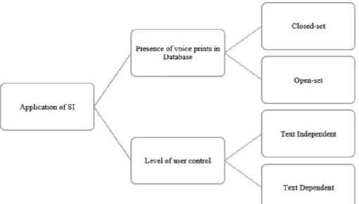
For this study, Tirumala et al. considered a simple classification of speaker identification techniques. The first level is divided into two parts – based on voiceprints and based on a new speaker with no voiceprints in the database. As shown in the fig 3, they are further divided into closed/open sets and text-dependent/independent approaches.
19
Figure 3: Types of speaker recognition
Along with classification, one major field of research in speaker recognition has always been the feature extraction phase. This is the phase where the enrollment of a speaker takes place and a copy of all data related to the speaker’s voiceprint is stored. As this can often be limited, the feature extraction phase becomes crucial in the overall speaker recognition model. Tirumala et al. have focused heavily on how deep learning can be used to overcome the difficulties faced in this phase. They designed a deep neural network (DNN) topology where every level works at the acoustic level. The training audio is fetched frame-by-frame and is fed to the DNN. Using this, the previous layer’s output is used as a representation for the particular speaker, called as the d-vector. These d-vectors are further used in DNN classifiers for speaker identification. Tirumala et al. proposed an architecture of using two DNNs with d-vectors and multiple hidden layers. This research does not showcase concrete results to compare their approach with traditional approaches, however, it serves as an initial stepping stone towards utilizing neural networks for feature extraction and classification in speaker identification.
Building upon the deep learning techniques discussed above for speaker recognition, Ge et al. researched further on how a feed-forward neural network could be effectively sued for text-independent speaker recognition [17]. They focused on using a unique technique of Voice Active Detection for feature extraction instead of the traditional techniques as this helps in eliminating the discrepancies that may be present in different audio samples for the same speaker. Additionally, they used MFCC on the preprocessed speech for normalization and concatenation.
20
They normalized the features using the mean and variance of the speaker with itself instead of using the values obtained on the entire dataset. This is known as Speaker Level MVN. For classification, they used the features comprising nearly 400-dimension vectors as inputs to the neural network and used Andrew Ng’s famous approach of considering a multi-class classification as n different binary classification, where n is the number of classes [11]. They ran their experiments on the TIMIT dataset using the first 200 male speakers for the training phase and used thresholding and ROC plots for verification. With this approach, they obtained decent accuracy rates and an Equal Error Rate of less than 6% which is impressive. The research marks a key progress in the usage of neural networks for speaker recognition, however, it is not evaluated on real-work natural environment sounds. Also, the training process is much slower as it requires more processing power and trains the model individually instead of considering a group of speakers as a whole.
21
3. Feature Extraction
As discussed earlier, speaker recognition is the process of recognizing who the person is using the person’s voiceprint. Thus, this research revolves heavily around sound processing and sampling of audio files. Any sound is composed of different frequencies, amplitude, wavelength, and many such related features - and it is important to quantify these characteristics of sound to perform experiments on them. However, it is also crucial to understand different sound features and the impact they have on the audio generated out from them.
In order to determine the sound features relevant to speech processing for speaker recognition, we first need to understand the different type of audio features. Audio features can be broadly classified into three types:
• Rhythmic features • Temporal features • Spectral features
Rhythmic features primarily deal with features related to musical notes and are heavily used in applications related to music information retrieval (MIR). Temporal features describe an audio signal over a sampled period of time. Few examples of temporal features are zero-crossing rate, minimum amplitude, or maximum frequency. These features are generally used in applications which deal with understanding the continuity of the audio signal – for instance, detecting a sudden change in oceanic wave sounds. Temporal features are sometimes also used in MIR while performing genre classification.
For speech processing, spectral features are considered to be most effective. Spectral features are based on the frequencies of the audio waves and are used for converting temporal features to equivalents domain of frequency [18]. This is very similar to how the human ear treats audio signals. The human ear receives the temporal signals, which are then converted to their frequency domains resulting in corresponding vibrations in the human ear giving us the ability to hear and comprehend an audio signal. Precisely for this reason of being very similar to how humans perceive audio, spectral features are the most widely used features in speech and speaker recognition systems.
There are several methods used for generating frequency domains for spectral features. Few of the notable ones used in speaker recognition are Linear Predictive Coding (LPC), Rastafilter, and Mel Frequency Cepstral Coefficients (MFCC). Studies suggest that MFCCs
22
represent the closest relation to the human earing model and are becoming increasingly popular in speech recognition. We shall thus have a look at MFCC in a bit more detail to understand know more about them and their respective variations. However, before studying about MFCCs, we first need to understand what framing an audio file means and why it is useful in feature extraction.
3.1. Audio Framing
As discussed earlier, an audio signal is a continuously changing collection of different frequencies bounded together. Hence, it is impractical to generalize the entire band of changing signal as one entity and to perform calculations on it. Instead, it is assumed that an audio signal does not change much over small intervals of 20 – 40 milliseconds. Thus, in an ideal scenario, the number of frames of an audio with frame length 20 milliseconds would be n = L / 20 where L is the length of audio in milliseconds and n is the number of frames. However, this is usually not the case. When an audio signal is framed, the edges become sharp and lose their true and harmonic nature. This is acceptable in learning about the short-term features and the frequencies of the frames, but we lose the continuity between adjacent frames which can misrepresent the audio frequencies. Thus, a concept of overlapping is used while framing audios. The overlapping length is usually defined by the hop size of the framing function. For instance, if a framing length of 25ms and hop length of 10ms is selected, the first frame would contain information about the frequencies between 0 – 25ms, the second frame would contain information about 10 – 35ms, the third will contain between 20 – 45ms and so on. Thus, as illustrated in the figure below, each frame has information about the latter half of the previous frame and the initial half of the next frame [19].
23
3.2. Mel Frequency Cepstral Coefficients (MFCC)
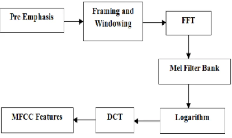
Mel Frequency Cepstral Coefficients are a set of spectral audio features which are effective in speaker recognition systems. P. Mermelstein, J.S. Bridle, and M.D. Brown are primarily credited for coming up with the idea of MFCCs [20]. MFCCs are a list of coefficients that in totality represent a Mel Frequency Cepstrum (MFC) [20]. The steps to identify the MFCCs are as follows:
1. Frame or window the signal into blocks that usually range between 20 - 40ms.
As discussed earlier, framing is essential before extracting features from the audios. However, unlike most application where a frame length of 20-40ms is considered fine, for speaker recognition systems, scientists have studied the frame length of up to 250ms can yield good results. Taking wider frames makes the frames less specific but also greatly reduces the total number of frames, thereby speeding up the overall process of feature extraction.
2. Perform a Discrete Fourier Transform (DFT) on this framed signal and calculate the powers of the spectrum.
Fourier transform is used to split the time-signal function into the multiple frequencies it is composed of. This step is motivated by the fact that the cochlea in human ear vibrates in different patterns and in multiple spots depending on the incoming frequency [21]. Assuming Si (k) denotes the DFT for the framed signal i and k denotes the DFT length, then the formula is:
S
i(k) =
∑
𝑵𝒏=𝟏s
i(n)h(n)e
-j2πkn/NWhere h(n) is an analysis window for the Nth sample.
Further, the spectrum power is calculated as Pi (k) = (1/N) | Si (k) |2
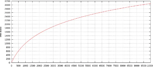
3. Map the above calculated power spectrums to the mel-scale.
The mel-scale represents the multiple pitch scales that an audio receiver or listener interprets. The formula to convert the hertz to mels is given as:
m = 2595 log
10(1 +
𝒇
𝟕𝟎𝟎
) = 1127 ln (1 +
𝒇 𝟕𝟎𝟎
)
24
Additionally, triangular overlapping filters are also used for the mapping. These are a set of 26 vectors and each is 257 in length. Every value of this filterbank is multiplied with the spectrum power calculated in the previous step followed by adding up the coefficients [21]. The mapping of these values is commonly called as the mel-scale as represented in the figure below [22].
Figure 5: Mel Scale
4. Compute the logarithm of energies
This step gives us the values of the filterbanks. It is obtained by taking the logarithms of the energies obtained in the previous step.
5. Finally, compute the discrete cosine transform (DCT) of the filterbank energies to get the MFCCs.
3.3 MFCC Delta: Differentials
Apart from the standard set of coefficients known as the MFCCs, there are variations of it that exist too. The most prominent ones are those which are obtained by calculating the deltas of the coefficients. They represent the path that the MFCCs encounter, which is known to increase
25
the accuracy of speech recognition researches in general. The first order MFCC deltas are sometimes also referred to as differentials.
The formula for calculating the MFCC delta coefficients is:
d
t=
∑𝑵𝒏=𝟏 𝒏(𝒄𝒕+𝒏− 𝒄𝒕−𝒏 ) 𝟐 ∑𝑵 𝒏𝟐
𝒏=𝟏
where, dt is the delta value coefficient for the window t, and c represents the MFCC coefficients.
3.4. MFCC Delta-Delta: Accelerations
Similarly, the MFCC delta-delta coefficients are calculated when the formula is applied on the MFCC delta coefficients. These are called as MFCC Delta-Delta coefficients, sometimes also referred to as accelerations. The formula for calculating the MFCC delta-delta coefficients is the same as MFCC delta coefficients with the only change being that here we use the delta coefficients instead of the original MFCC coefficients. Thus, the formula is
dd
t=
∑𝑵𝒏=𝟏 𝒏(𝒅𝒕+𝒏− 𝒅𝒕−𝒏 ) 𝟐 ∑𝑵 𝒏𝟐
𝒏=𝟏
where ddt is the delta-delta coefficient for window t, and dt represents the MFCC delta coefficients. For simplicity, the MFCC delta-delta calculation can also be represented as follows:
MFCC delta-delta = Δ (MFCC delta) = Δ (Δ (MFCC))) where Δ represents the delta function.
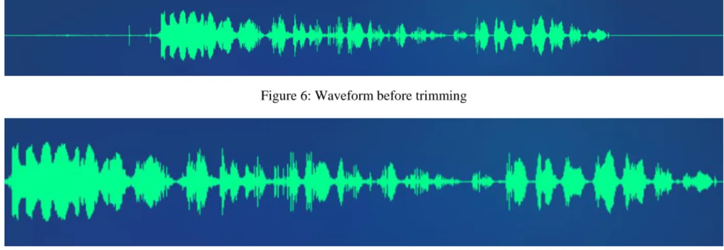
3.5. Edge Trimming
As discussed earlier, MFCCs and their derivates are obtained by dividing an audio into small frames ranging from 20ms – 250ms. While this approach sounds effective, it presents one major problem of calculating coefficients of unwanted frames. Unwanted frames are simply the frames, often at the beginning and at the end of a sentence which do not contain any useful information. This usually happens due to the delay in the time taken to stop the recording after a speaker completes his sentence. To compensate for this, the concept of audio edge trimming is adopted by researchers. Edge of an audio is defined as the starting and the ending part of it, similar to trailing and leading spaces in textual data. There are different ways to remove the unwanted trailing, but usually a threshold value in decibel is set and a value below that is considered silence. The average decibel value for each frame is calculated and if the value is below the threshold, the
26
edge is trimmed. Fig 6 represents a sample waveform containing the silent edges and Fig 7 shows the waveform after edge trimming.
Figure 6: Waveform before trimming
27
4. Machine Learning Classifiers
Similar to the feature extraction techniques, the machine learning classifiers also play a vital role in determining the overall effectiveness of speaker recognition model. As we have an intention to classify audios and determine the speaker in them, this is a classification problem and hence we shall discuss about some effective supervised classification machine learning algorithms.
4.1. Support Vector Machine (SVM)
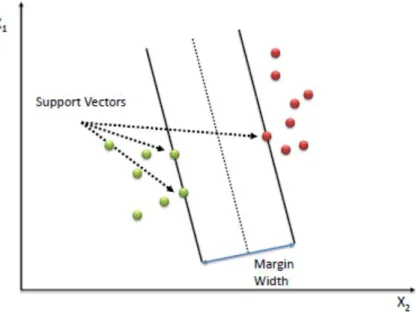
Support Vector Machine, sometimes abbreviated as SVM or SVC (Support Vector Classifier) is a well-known supervised machine learning classification technique. The objective of a SVM algorithm is to construct an n-dimensional hyperplane which can be used for classification or regression. Ideally, a good hyperplane is the one that achieves the largest distance to the closest data point of a particular class [23]. This can be better explained with the help of fig 8 [24].
Figure 8: Sample hyperplane for binary classification
Here, the red and green dots represent two different classes of the dataset. The support vectors are the points which help in identifying the hyperplane, and in this scatterplot, the green class provides two support vectors and the red class provides one. Using these support vectors, we draw lines passing through them that would distinguish the data from the other class.
28
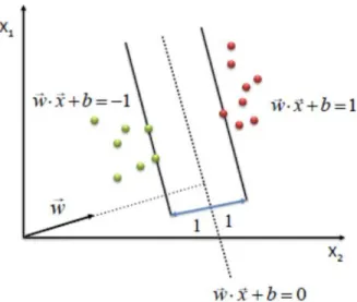
Figure 9: Generation of the hyperplane using support vectors
Doing this, we get the two lines w*x + b=1 and w*x + b=-1. Additionally, these two classes are linearly separable and plotting the hyperplane is straightforward in this case. A hyperplane is simply a straight line which divides the two classes with a maximum distance from the points closest to the line, also known as the support vector. However, the essential part of a SVM is to define an optimal hyperplane that would maximize the margin width (w). In an ideal scenario, the maximum width is obtained by the formula 2
∥𝑤∥ .
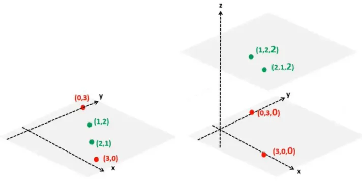
However, for most scenarios, the data is not scattered in a manner that would be linearly separable. Also, a line might not be used for always defining the hyperplane. A plane can be used as the hyperplane in spaces with higher dimensions. Additionally, the data might not always be linearly separable. For a non-linear distribution of data, SVM has a concept of kernel trick which is used for defining the optimal hyperplane. The kernel trick converts the given data into a higher dimensionality space to achieve a linear separation between the points. Fig 10 shows how the hyperplane changes from a line (x,y) to a plane (x, y, xy) depending on the dimensionality space.
29
Figure 10: Linear hyperplane vs hyperplane generated using a kernel trick
Fig 10 represents a simple kernel function which used the formula x,y,x*y to obtain a linear separation of data. This is a simple representation of how kernel tricks work. The Gaussian Radial Basis Function (RBF) is the most widely used kernel trick in SVM and it is defined by the following equation:
SVMs were primarily used for binary classification problems, however, the recent developments in kernel tricks have made them efficient for multiclass classifications too. They use the ‘One vs All’ (OvA) technique while performing the classification on each class during a multiclass classification. For instance, let us assume there are three classes – A, B, and C and an input x is to be determined. The SVM will first check x for class A as ‘A vs non-A’ and calculate a score. Similarly, it does the same for ‘B vs non-B’ and ‘C vs non-C’ to get multiple scores. These scores are then ranked to determine the classification of the input x.
30
4.2. Random Forest Classifier
Random Forest Classification (RFC) is another supervised classification technique based on decision trees used in machine learning. A decision tree algorithm builds a tree-like model of the dataset where each node is split further based on several customizable criterion [25]. A Random Forest is a collection of unbiased, unrelated, and de-correlated decision trees and hence are named as a ‘random forest’. Before we discuss about random forests, we first need to understand what a decision tree and how it works.
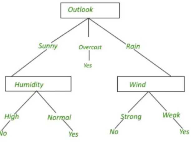
A decision tree is a collection of connected nodes where each node is reachable from the previous node depending on certain criteria. For instance, assuming a person wants to go for a picnic but is unable to determine if the day is suitable for it, then a decision tree might look like Fig 11 [26].
Figure 11: A simple decision tree illustration
The first node ‘Outlook’ is split into three conditions, namely ‘Sunny’, ‘Overcast’, and ‘Rain’ followed by more nodes below them. This is a very simple representation of the decision tree. Once a decision tree is created, it is fairly straightforward for the algorithm to classify the provided input sample by simply traversing the tree. However, there is no perfect decision tree that exists for a dataset. There are different methods using which the splits at every node can be mode and that largely affect the decision tree formation. For instance, the decision tree would look very different if the first node was ‘Wind’, instead of ‘Outlook’. The performance of the decision tree would also change significantly based on this design change. Hence, it is imperative to know the factors that affect determining the current node and the splitting criteria.
31
The two most significant concepts that are widely used for this determination are Gini and Entropy values. Gini is used to calculate the impurity and Entropy is used for calculating the information gain of the node. Hence, while calculating the Gini impurity, the node that provides the least Gini impurity is selected for the split. The formula for calculating the impurity from the Gini value is defined as 1 minus the square of the probability of each class. Symbolically, it can be represented as: . A perfect split would result in the Gini score of 0, which would always be the case at the leaf nodes.
Similarly, while using Entropy, the goal is to split at the node which provides the maximum information gain. At the leaf node of three, Entropy gain is 1 which means full information gain and is thus is a perfect split. Entropy is calculated using the formula E(S) = ∑𝑐𝑖=1− pi log2 pi. Based on this value, we calculate information gain as the difference between the other classes and the calculated entropy. The information gain for each is then compared the split providing the maximum gain is selected as the splitting criteria.
The primary difference between Gini and Entropy is that Gini is usually used to minimize misclassifications whereas Entropy is used more for exploratory purposes. Hence, Gini is usually considered a good measure for classification problems. Another difference is that Entropy is usually slower to compute due to logarithmic operations.
Furthermore, all these computations are performed to determine just one decision tree. As discussed earlier, Random Forest is a collection of unrelated decision trees which can be created either by using the Gini or the Entropy values. Based on these specifics, the algorithm builds a forest of n trees. Assuming there are 3 classes – A, B, and C in a dataset and the forest contains 10 trees. Let us assume three trees predict the class as A, five trees predict the class as B, and remaining two trees predict the class C. In this case, the overall prediction of the Random Forest would be class B as that has the highest number of votes - five.
However, this problem can also sometimes lead to overfitting as those five trees might be biased towards class B, resulting in most predictions of the forest in B. Thus, increasing the number of trees greatly reduces the problem of overfitting in Random Forest Classification.
Thus, Random Forests are considered one of the best supervised classification algorithms as they make use of multiple decision trees that not only provides better classification but also avoid overfitting.
32
4.3. k Nearest Neighbors
The k Nearest Neighbors (kNN) algorithm for classification is one of the simplest machine learning classification algorithms. As opposed to most techniques, kNN is a lazy technique which means that it does the evaluations only when needed. This makes this algorithm fast at the cost of some accuracy. When an input is provided, kNN computes its distance with each vector in the dataset and then determines k vectors with the smallest distances. The classes of these kvectors are then compared and the class that was is predicted the most is returned. Although this approach sounds simple, it is effective in a lot of machine learning algorithms. The two most important decisions in this algorithm are the k value estimation and the distance metric.
The kvalue estimation is usually done using the elbow method which tries to find that value of k after which the accuracy does not increase much. The elbow method k value estimation thus gives a good k value with respect to time vs accuracy. Additionally, the two most widely used distance metrics for kNN are Euclidean Distance and Cosine Similarity. Usually, with continuous numbers such as the MFCC coefficients, the Euclidean distance is a more effective metric to choose as that compares the magnitude of difference between the vectors. Cosine similarity also calculates the difference in the vector direction which is not required for most studies. Mathematically, Euclidean distance is calculated as:
33
5. Dataset
When working on a speaker recognition study, the dataset is of utmost importance as the audios must be of a certain quality in order to perform experiments. Thus, most publicly available audio datasets are usually recorded in constraint sound-proof environments to maximize the effectiveness of the study. However, this is not the case in real life, especially when people use handheld devices such as mobile phones or tablet PCs to interact with the computer. Real life scenarios would often have background noise in the background. Noise need not always be a different sound, but just the ambient noise in the background is sufficient enough to reduce the effectiveness of feature extraction and subsequent classification techniques. However, although the ambient noises are a major hurdle in sound related studies, they are an inevitable reality and thus we wanted to focus on such scenarios for this research purpose. The primary motivation behind this is to simulate real life-like audio samples for the training and testing phases.
5.1 VoxCeleb Dataset
VoxCeleb is a recently published publicly available dataset which serves this purpose appropriately [27]. J.S. Chung, A. Nagrani, and A. Zisserman from the University of Oxford in UK published the dataset in 2017. As the dataset is not even more than 2 years old, it remains pretty unexplored and thus makes this research more interest. Moreover, the fact that it does not try to simulate an unconstrained environment but instead uses actual real-life footage makes this dataset more practical to work on. Thus, to summarize, the two primary reasons we believe that this is an appropriate dataset for this study are its freshness and its closeness to real-world scenarios.
The two most common audio formats that exist presently are WAV and MP3. For most researches, WAV files are considered more useful as they cover the entire range of frequencies that are audible to the human ear. On the other hand, MP3 files are compressed and hence do not contain all the information that is usually encompassed in a WAV file of the corresponding audio. Additionally, feature extraction from these WAV files is extremely crucial. This phase essentially forms the basis of the machine learning algorithms to be used for classification. Thus, WAV files are largely preferred audio studies, and VoxCeleb does a great job of providing WAV files at constant sampling rates. Sampling rate is defined as the absolute number of audio samples present in one second [28]. Consistency in sampling rate is very important in an audio study to ensure that
34
the extracted coefficients represent the same underlying calculations. Hence, this is another reason why VoxCeleb dataset is apt for this study as it has sampled all audios to a constant sampling rate of 16000 Hz.
5.2. Dataset Diversity
For the purpose of this study, we have selected 40 speakers to evaluate our models on. The primary factors behind the selection of these 40 speakers were:
1. To have an equal number of male and female speakers: This avoids overfitting the training and testing techniques for a particular gender.
2. To have different accents: We have selected people from different nationalities to obtain a variation in the accents they speak in.
3. To have multiple languages: As the research is based on text-independent approach, we can not only have people with different accents but can have people speaking altogether different languages. This simulates a more real-life scenario as the model will not be evaluated on just one specific language.
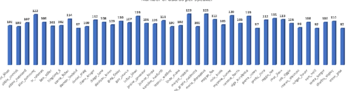
Keeping these factors in mind, we obtained more than 4300 audio files to train the model on. Each audio file ranges between 5 seconds to 20 seconds, with approximately 100 audios per speaker. However, when a speaker recognition system is developed in real-life, the case may not be so perfect. It is common to have more samples of audios for one speaker and lesser number of samples for another. Hence, to simulate this real-life imbalance which is extremely common, we have ensured that we have a slightly varying number of audio samples for each person to train the model on. This not only enables us to test the flexibility of the models but also gives us an idea if the true positive rate for a speaker changes with the number of samples, and if yes, then by what extent.
Fig 12 shows the number of audio files used per speaker for the study.
35
Figure 13: Nationality distribution of speakers
Below is a brief overview of the diversity of the dataset: 1. Genders: 50% Male, 50% Female
2. Nationalities: Australia, Austria, Canada, China, Germany, India, Italy, Mexico, Netherlands, New Zealand, Norway, Philippines, Poland, Russia, South Africa, Spain, Sweden, United Kingdom, United States of America
3. Languages: English, French, German, Hindi, Russian, Serbian, Spanish, Tamil
Additionally, the dataset also contains several types of background noise in the collected 4300 audio files. Ambient noise is the most common of them all, however, there are cases of motor-vehicle sounds, speeches of other people, music, applause, motor-vehicle honking sounds also present in the audio files. This makes up for an interesting study as the ambient noise removal algorithm that we have implemented will be evaluated on different kinds of background noises.
36
6. Tools and Libraries
6.1. LibROSA
LibROSA is a Python library built for sound analysis [29]. It is considered as one of the most versatile libraries for audio processing in Python. It provides a plethora of useful sound processing features as waveform visualization, feature extractions, math operations, and a few more. It also has in-built IPython sound widgets which make it easier to debug the sound processing phase.
6.2. python_speech_features
Similar to LibROSA, even python_speech_features is a library having multiple built-in audio processing methods related to feature engineering [30]. It provides methods to extract the MFCCs, filterbank energies, spectral centroids, and also logarithmic filterbank energies. The spectral centroids computing method is very effective in the approach we have taken to eliminate ambient noise during the audio pre-processing phase.
6.3. Scikit-learn
Scikit-learn (also known as sklearn) is an efficient and well-known library built for Machine Learning in Python. It provides methods for several machine learning and data mining tasks such as regression, classification, clustering, modelling, and several other machine learning activities. We have used sklearn for several tasks such as normalization, scaling the data, building classification models, generating cross-validations, evaluating the model performance, and visualizing the results.
6.4. Other Python libraries:
Apart from the libraries mentioned above, few other third-party Python libraries used for the implementation are: Scipy, NumPy, Pandas, Matplotlib, Seaborn, and Pysndfx.
37
7. Implementation
As discussed in the feature extraction part of the report earlier, the phases related to audio pre-processing and feature extraction are critical in designing a good speaker classification model. Also, as discussed in the dataset part of the report earlier, the audio files used for this dataset are not recorded in a constrained environment and contain some noise, usually ambient, and some abrupt pauses between words sentences which are not useful for the feature engineering of audio. Hence, we first pre-process the audio and do the MFCC feature extraction in order to ensure that our extracted features represent the audios with higher accuracy.
Fig 14 represents the steps we have taken during the feature extraction phase. They include processes such as:
• Ambient noise reduction • Vocal enhancements • Audio trimming • Audio splitting
• MFCC Feature Extraction
Figure 14: Audio pre-processing and feature extraction
7.1. Ambient Noise Reduction
Ambient noise is defined as any noise which exists in the background of the environment. Although present in the background, these ambient noises can have severe ill effects in understanding the features of the audio. Hence, it is essential to reduce the ambient noise as much as possible to ensure better feature engineering.
38
1. Divide the audio in frames of 25ms with hop length of 10ms.
2. Calculate the spectral centroids for each window. This is achieved by using the method features.spectral_centroid() of LibROSA.
3. Determine the maximum and minimum centroid value from the values calculated in the previous step. Let us call them the upper and lower thresholds respectively.
4. Apply a lowshelf filter for gain=-30 and frequency as the lower threshold. The lower threshold points towards the noisy part of the audio, and setting the gain to -30 significantly reduces those volumes which eventually helps in reducing those signals in the audio. Lesser gain reduces volume, eliminates insignificant noises.
5. Now, apply a highshelf filter for gain=-30 and higher threshold. This step is practically useful in reducing the foreground noises that might exist in the audio. For example, a person clapping close the mic between the speech of a person can be classified as a foreground noise.
6. To compensate for the volume loss in steps 4 and step 5, we apply limiter with a gain of +10 to increase the volume.
7.2. Vocal Enhancement
Unlike ambient noise, vocal and voice signals are the features that we want our feature extraction phase to focus more on. These are the significant parts of the audio that we wish to use to extract features from and build machine learning classifiers. Hence, enhancing these parts of the audio can greatly increase our accuracies. We can do this by using the concepts of MFCCs again. Following are the steps we took to enhance the vocal enhancements.
1. Divide the audio in frames of 25ms with a hop length of 10ms. 2. Calculate the MFCC coefficients for each frame.
3. Take the sum of squares of MFCC. Squaring the coefficients greatly helps in summarizing the spread of data. Additionally, MFCCs might not always be positive, squaring makes sure that all comparisons are made in the positive space of numbers. Although this can be achieved by absolute values too, squaring helps in summarizing the spread in a better way. 4. Find the strongest frame. The strongest frame is the frame which has the maximum sum of squares for its MFCCs. The reason for taking the strongest frame is that would indicate a certain vocal utterance. This is because we do this step after ambient noise removal, which