A University of Sussex PhD thesis
Available
online
via
Sussex
Research
Online:
http://sro.sussex.ac.uk/
This
thesis
is
protected
by
copyright
which
belongs
to
the
author.
This
thesis
cannot
be
reproduced
or
quoted
extensively
from
without
first
obtaining
permission
in
writing
from
the
Author
The
content
must
not
be
changed
in
any
way
or
sold
commercially
in
any
format
or
medium
without
the
formal
permission
of
the
Author
When
referring
to
this
work,
full
bibliographic
details
including
the
author,
title,
awarding
institution
and
date
of
the
thesis
must
be
given
Features
Joseph Gerard Taylor
Submitted for the degree of Doctor of Philosophy University of Sussex
Declaration
I hereby declare that this thesis has not been and will not be submitted in whole or in part to another University for the award of any other degree.
Signature:
UNIVERSITY OF SUSSEX
Joseph Gerard Taylor
Submitted for the degree of Doctor of Philosophy
Privileged Learning Using Unselected Featurers
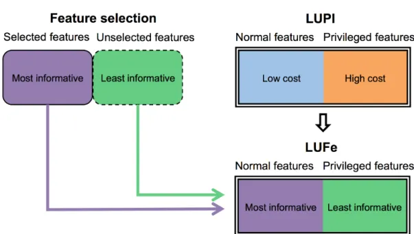
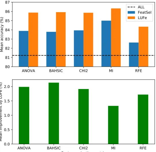
This thesis proposes a novel machine learning paradigm called Learning using Unselec-ted Features (LUFe), which front-loads computation to training time in order to improve classifier performance, without additional cost at deployment. This is achieved by re-purposing and combining techniques from feature selection and Learning Using Privileged Information (LUPI). Feature selection is a means of reducing model complexity, which enables deployment in devices with limited computational power, but this can waste addi-tional resources which may be available at training time. LUPI is a paradigm that allows extra information about the training data to be harnessed by the learner, but this requires an additional set of highly informative attributes. In the LUFe setting, feature selection is used to partition datasets into primary and secondary subsets, instead of discarding the features which are unselected. Both datasets are then passed to a LUPI algorithm, enabling the secondary feature-set to provide additional guidance at training time only, in place of ‘privileged’ information. Only the selected features are used at train time, maintaining low-cost deployment while exploiting train-time resources.
Experimental results on a large number of datasets demonstrate that LUFe facilitates an improvement in classification accuracy over standard feature selection approaches in a majority of cases. This performance boost is consistent across a range of feature selection approaches, and is largest when the SVM+ algorithm is used for implementation. This effect is shown to be partially dependent on the usage of information in the unselected features, as well as resulting from the presence of additional constraints on the function space searched for the model. The enhancement by LUFe is shown to be inversely cor-related with the performance of standard feature selection and mediated by a further reduction in model variance, beyond that provided by standard feature selection. Aside from demonstrating the direct practical benefit of LUFe, this work makes the contribution of broadening the scope of applications for the LUPI framework.
Acknowledgements
I would like to start by thanking my family for all their constant encouragement: my parents Ged and Marian, my sister Dee, my niece Hannah, and my nephews Alfie and Alex. Thank-you to my wonderful partner Clemy who has been amazing and supportive of me. Thanks to everyone I have shared an office with, and last but not least, thanks to my supervisors Novi and David.
Contents
1 Introduction 2
1.1 Classification with limited resources . . . 2
1.2 The basis for this research: LUPI and feature selection . . . 3
1.2.1 Limitations of current work . . . 4
1.3 Introducing LUFe: hypothesis and research questions . . . 4
1.4 Outline . . . 5
1.5 Summary of contributions . . . 6
1.6 Outline of publications . . . 7
2 Background 8 2.1 Learning Using Privileged Information . . . 8
2.1.1 Motivation for Learning Using Privileged Information . . . 9
2.1.2 LUPI in context . . . 11
2.1.3 Technical explanation of LUPI . . . 11
2.1.4 SVM . . . 12 2.1.5 Oracle function . . . 16 2.1.6 SVM+ . . . 17 2.1.7 dSVM+ . . . 22 2.1.8 SVM∆+ . . . 23 2.1.9 Margin Transfer . . . 25
2.1.10 Beyond supervised learning: GPC+ . . . 27
2.1.11 Beyond classification: unsupervised LUPI . . . 27
2.1.12 Assessing SVM+ performance. . . 28
2.1.13 Questioning the mechanism of LUPI . . . 29
2.1.14 Comparison to other approaches . . . 30
2.2 Feature Selection . . . 32
2.2.2 Wrapper methods . . . 34
2.2.3 Embedded methods . . . 35
2.2.4 Combining methods . . . 36
2.2.5 Comparing approaches in the context of this thesis . . . 36
3 Related work 38 3.1 Using the variables that machine learning discards . . . 38
3.1.1 Unselected features in multi-task learning . . . 38
3.1.2 Comparison with LUFe . . . 39
3.1.3 Experimentation . . . 39
3.1.4 Concluding remarks . . . 41
3.2 Other approaches to front-loading training . . . 43
3.2.1 Model compression . . . 43
3.2.2 Distillation . . . 44
3.2.3 Unifying distillation and privileged information . . . 45
3.3 Other approaches with different information at train and test times. . . 46
3.3.1 Domain adaptation. . . 47
3.3.2 Transfer learning . . . 49
3.3.3 Multi-view learning . . . 51
4 Learning using Unselected Features 53 4.1 Overview . . . 53
4.2 Motivation . . . 54
4.2.1 Use cases . . . 55
4.2.2 Feature selection revisited . . . 57
4.2.3 Rethinking feature selection . . . 59
4.2.4 Comparison with LUPI and conventional feature selection . . . 61
4.3 Experimentation . . . 62 4.3.1 Dataset . . . 63 4.3.2 Experimental protocol . . . 64 4.3.3 Implementation. . . 66 4.3.4 Results . . . 66 4.3.5 Discussion of results . . . 76
4.4 Further analysis of results . . . 77
4.4.2 Dataset topics and distance . . . 80
4.5 Further experimentation 1: Altering the number of selected features . . . 84
4.5.1 Experimentation . . . 84
4.5.2 Results and discussion . . . 84
4.6 Further experimentation 2: Comparison with Existing Method to Utilise Discarded Features . . . 86
4.6.1 Experimental procedure . . . 87
4.6.2 Results . . . 89
4.6.3 Discussion. . . 89
4.6.4 Closing remarks . . . 94
5 Further Investigating Unselected Features 95 5.1 Feature selection methods . . . 96
5.1.1 Comparison of filter and wrapper methods. . . 96
5.1.2 Experimental procedure . . . 97
5.1.3 Results . . . 98
5.1.4 Discussion. . . 101
5.1.5 Further analysis of results . . . 102
5.1.6 Further experimentation A: Comparison with multi-task learning . . 110
5.1.7 Further experimentation B: RFE step-size parameter . . . 111
5.2 Alternative implementations of LUPI . . . 114
5.2.1 SVM∆+ . . . 114
5.2.2 dSVM+ . . . 115
5.2.3 Experimentation with different implementations . . . 116
5.2.4 Experimental procedure . . . 116
5.2.5 Results . . . 116
5.2.6 Discussion. . . 117
5.3 Using subsets of unselected features . . . 119
5.3.1 Methodology . . . 120
5.3.2 Results . . . 121
5.3.3 Discussion. . . 121
6 Investigating the mechanism of action for LUFe 125 6.1 Is LUFe dependent on Unselected Features? . . . 126
6.1.1 Experimentation . . . 126
6.1.2 Results . . . 128
6.1.3 Discussion. . . 131
6.1.4 Further experimentation: Random feature selection. . . 132
6.2 Assessing the value of unselected features . . . 134
6.2.1 Informativeness between feature sets . . . 134
6.2.2 Informativeness of individual feature sets . . . 135
6.2.3 Experimentation . . . 136
6.2.4 Results . . . 138
6.3 How does the LUFe setting improve performance? . . . 148
6.3.1 Learning curves. . . 148 6.3.2 Experimentation . . . 148 6.3.3 Discussion. . . 150 7 Conclusion 153 7.1 Summary of results . . . 153 7.2 Limitations . . . 154
7.2.1 Limitations to the scope of findings. . . 154
7.2.2 Limitations of applications for LUFe . . . 155
7.2.3 Limitations of assessment methods . . . 155
7.3 Further work . . . 156
7.3.1 Further work to address limitations. . . 156
7.3.2 Other areas for further work . . . 156
7.4 Closing remarks. . . 157
Preface
This thesis is the result of work carried out in the Text Analytics Group and Predictive Analytics Laboratory, in the Department of Informatics at the University of Sussex. An
earlier version of Chapter4 was published as Learning using Unselected Features (LUFe),
in the proceedings of the Twenty-Fifth International Joint Conference on Artificial Intel-ligence, IJCAI 2016, New York, NY, USA, 9-15 July 2016.
Chapter 1
Introduction
1.1
Classification with limited resources
The modern world is a data-rich environment, and suitable tools to understand, categorise and classify this data are more necessary now than ever. One general approach is machine learning. This broad term encompasses methods that enable systems to learn to perform a task from data, without requiring specific instructions. As computing becomes more pervasive, more devices and sensors require the capability to perform ‘intelligent’ tasks. Training the model may be centralised, and have access to great computational resources,
but at deployment, the model may have access to limited resources only (Hinton et al.,
2015). The need therefore rises for ‘asymmetrical’ systems, which allow a model to exploit
additional train-time resources, which are not required at deployment time — effectively ‘front-loading’ the burden of computation.
As an illustrative example, consider the case of a sensor array on an autonomous robot, which performs some initial processing to inform the robot’s actions — such as identifying and classifying an object. In this environment, each sensing unit must be able to respond to a constant stream of data and produce output with very low latency. The model in this scenario therefore requires the ability to handle high data velocity with a fast response rate. A smaller, less complex model built on fewer features would typically provide this, but it may be at the expense of accuracy. However, if this lighter-weight model were trained on a larger feature set offline before deployment, perhaps the accuracy could be improved while maintaining the rapid deployment time. It is this insight which motivates the work in this thesis. The purpose of this work, then, is to introduce, validate and examine a new learning paradigm called Learning using Unselected Features (LUFe), which is designed to improve classifier performance without increasing computational cost
at deployment time.
This thesis will focus on the task of classification, which is among the most common types of function that can be accomplished via machine learning. Classification involves learning to correctly assign a label indicating class membership to data points. and can
be applied to countless domains, including textual data, images, or financial data (Bishop
et al., 2006). Machine learning is typically categorised into two broad categories: su-pervised learning which learns from examples of input-output pairs, and unsupervised learning, which finds structure from input data without an associated output. Classifica-tion is usually handled as a supervised learning task, which takes pairs of training input feature vectors with output class labels, and learns a function that attempts to map each input vector to its corresponding label. Once learned, the function can then be applied to classify a new data point, by assigning it a label.
Recently, methods such as model distillation (Hinton et al., 2015) and model
com-pression (Bucilu˘a et al., 2006) have been developed in order to allow a relatively small
neural network to learn from a larger, more complex neural network-based model. These approaches allow the usage of a high-performing model with low deployment cost. This thesis presents a related but novel manner of front-loading the computational cost of a model, with a focus on SVM-based classification.
1.2
The basis for this research: LUPI and feature selection
This thesis builds upon two existing machine learning methods: Learning Using Priv-ileged Information (LUPI) and Feature Selection. Learning Using PrivPriv-ileged Information is a relatively novel paradigm that allows additional, highly informative (‘privileged’) in-formation about training instances to be harnessed during training, even though equivalent
information will not be accessible for unseen instances at deployment time (Vapnik and
Vashist, 2009). The privileged information is typically from a different domain and rep-resented in a separate feature space. Given that the privileged information is not available at deployment time, it is harnessed through a ‘teacher function’ that guides the ‘student function’ to learn a better decision function in the standard feature space. This is accom-plished by improving the student function’s convergence rate to the optimal solution. For a given amount of training data, a faster-converging solution will get closer to the optimal solution.
Feature selection is a widely-used approach to reduce model size, that is employed in a
involves selecting a subset of the most relevant attributes from the available dataset, and typically using only this subset in modelling of the problem. Feature selection produces benefits including improvements to human interpretability, to the cost of storage and data collection, and to the computational cost of training and deploying the model. It can also improve model performance by reducing variance, and preventing overfitting to noisy or irrelevant attributes. Approaches to feature selection are usually grouped into ‘filter’, ‘wrapper’ and ‘embedded’ types, based on how they approach this task.
1.2.1 Limitations of current work
Existing research on LUPI and feature selection approaches has certain limitations, which are addressed by the work in this thesis. LUPI is an exciting and powerful method of boosting performance compared to conventional supervised learning, but requires a spe-cific scenario: a supervised learning task to be performed, with a standard dataset, and an additional, highly informative dataset which is available for all training instances. Its application has therefore been limited to those settings where a secondary dataset, provid-ing an alternate ‘view’, is accessible for trainprovid-ing instances. However, as a relatively new learning setting, there remains a lack of empirical work to validate that LUPI actually requires a highly-informative secondary data set, as the literature describes.
Feature selection is effective at reducing model complexity but may lose information contained in the discarded features. This is particularly an issue in filter and wrapper approaches, which discard all attributes that are not included in the selected subset passed
to the learner. Feature selection is an NP-hard problem (Weston et al., 2003), so most
approaches tend to generate a sub-optimal feature set, and therefore lose information in the unselected features. Even if feature selection were to perform optimally, there remains a trade-off between size of the selected subset and model performance.
1.3
Introducing LUFe: hypothesis and research questions
This setting involves a novel combination of LUPI and feature selection, based on the insights from the previous section that (a) the LUPI framework may be under-used and more broadly applicable and (b) standard feature selection approaches tend to be sub-optimal. This is used to address the previous observation that front-loading computation has practical benefits. To summarise this approach: a standard feature selection algorithm is performed to partition the dataset into ‘selected’ and ‘unselected’ subsets, which are both then supplied to an implementation of LUPI. The selected features are supplied as
the primary feature set, to be used at both train time and deployment time, and the unselected features are passed in place of the ‘privileged’ features, for training data only. In this manner, both LUPI and feature selection are repurposed: feature selection is now used to split the data into subsets of ‘primary’ and ‘secondary’ importance, rather than being used to assign useful and discarded feature sets. The LUPI framework is broadened in scope, and its use-case extended; the secondary dataset may now consist
of features which have been assigned as less informative attributes of the same domain
by the feature selection process, rather than more informative attributes from a different domain.
The benefit of this research is twofold. Firstly, the practical application of LUFe allows model accuracy to be boosted with no additional cost at deployment time. This effectively allows computation to be ‘front-loaded’, with more computational resources exploited at training time in order to learn a better model, but without additional cost when the model is being deployed. The second benefit is to question the theoretical underpinning of the
LUPI framework. The expansion of this paradigm by using a less informative secondary
feature set to improve performance demonstrates that the LUPI model is not entirely dependent on the availability of highly informative ‘privileged’ information, as described in the majority of literature on this topic.
The research asks the following questions. Firstly, whether the LUPI framework can be re-purposed to improve model performance by using unselected features — rather than privileged information. Secondly, whether the performance of LUFe is consistent when implemented using different LUPI algorithms, and when the primary and secondary inputs are assigned by different feature selection algorithms. Thirdly, whether any improvement due to LUFe is actually dependent on information contained in the unselected features, and how this benefit is accomplished.
1.4
Outline
This thesis begins with a two-part chapter which summarises the main areas of background work which LUFe builds upon. The first part describes the state of current research on LUPI, describing the motivation for this framework, the technical details of various LUPI implementations, and reporting some experimental results achieved using this paradigm. The second part describes the three main categories of established approaches to feature selection, and describes the benefits and challenges associated with each. The second chapter then continues to review the literature, describing other related work: namely,
existing approaches taken to front-load computation, and more broadly, other work which takes an asymmetric view of the data at train time and deployment time.
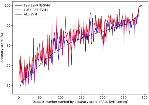
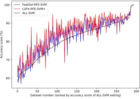
The following three substantive chapters each then contain the main contributions of this work. Firstly, the LUFe paradigm is introduced, along with motivation and theoretical justification, and an experimental framework to test its efficacy is described. This is used to provide proof-of-concept experimentation, where LUFe is shown to provide a performance boost in a majority of classification tasks on 295 datasets.
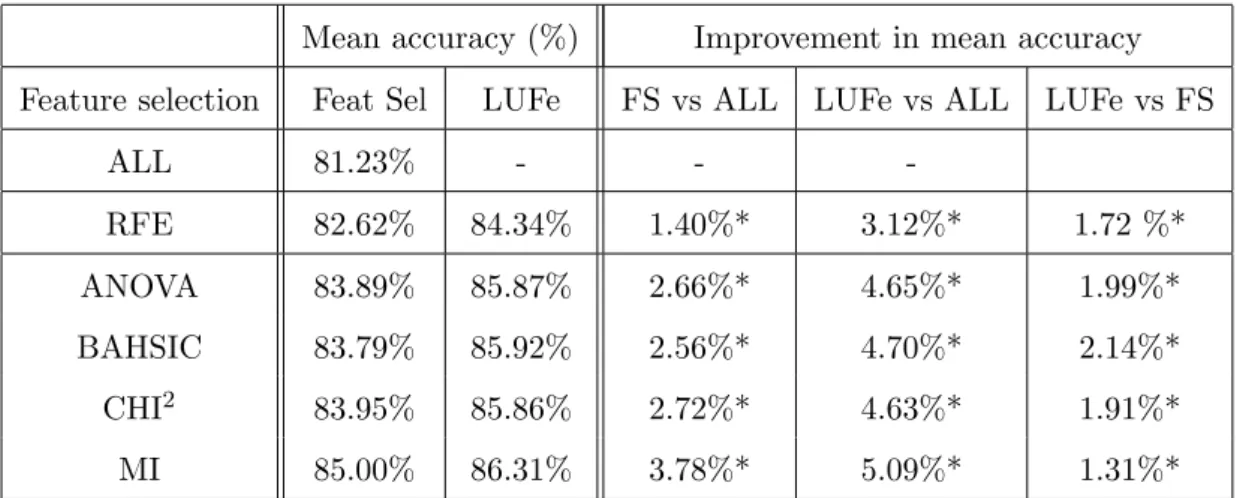
Secondly, the LUFe framework is examined in a wider range of settings: its perform-ance is assessed in combination with a range of feature selection methods, with different implementations of the LUPI paradigm, and with different subsets of unselected features. The performance boost due to LUFe is shown to be robust across a range of different feature selection methods, but performance is affected by the choice of LUPI algorithm for implementation.
The third substantive chapter then investigates the mechanism by which LUFe works. LUFe is compared with performance using ‘dummy’ datasets to assess the impact of the
unselected features. Metrics to predict the LUFe performance boosta priori are described
and tested. Learning curves are used to investigate the effect of LUFe on the bias-variance trade-off. The implications for the LUPI framework are discussed.
Conclusions, interpretations, limitations, and areas for future work are then discussed in a final chapter.
1.5
Summary of contributions
The contributions of this thesis are summarised as follows:
1. The introduction of the Learning using Unselected Features (LUFe) paradigm, to improve classifier performance in scenarios with limited resources at deployment, by front-loading computation to training time
2. The novel combination of Learning Using Privileged Information (LUPI) with feature selection, which repurposes LUPI algorithms to use a less informative secondary feature set
3. Validation of LUFe performance from experimental results on 295 datasets, demon-strating a robust improvement that is dependent on the implementations of feature selection, and of LUPI
4. Experimentation that investigates the mechanism of action for LUFe, demonstrating a dependence on the efficacy of feature selection
1.6
Outline of publications
The following publication resulted from this thesis:
• Taylor, J., Sharmanska, V., Kersting, K., Weir, D., and Quadrianto, N. (2016).
Learning using Unselected Features (LUFe). In Proceedings of the Twenty-Fifth International Joint 144 Conference on Artificial Intelligence, IJCAI 2016, New York, NY, USA, 9-15 July 2016. AAAI Press/International Joint Conferences on Artificial Intelligence. 56
Chapter 2
Background
The work in this thesis bridges a gap between two distinct topics in machine learning:
Feature Selection and Learning Using Privileged Information. The intersection
of these fields is a novel area of research, so the background material will be described in terms of these topics as two discrete sections.
2.1
Learning Using Privileged Information
Learning Using Privileged Information (LUPI) is a machine learning paradigm that can improve performance by incorporating some additional information when training a model,
which is not available at test time (Vapnik and Vashist, 2009).1 This section will first
provide a high-level description of the motivating concepts for the LUPI framework, with particular focus on its usage in the supervised classification setting which is most relevant to this thesis. Then the technical details underlying LUPI will be tackled in more depth: firstly, the general principles of supervised classification and specifically the support vector machine (SVM) classifier are reviewed. This will lay the groundwork to then explain how the SVM+ instantiation of the LUPI paradigm can employ additional information to improve upon this performance. Alternative LUPI implementations are discussed, such
as dSVM+, SVM∆+ and GPC+. Finally, some experimental results using LUPI are
described.
1
This kind of learning was first described in the afterword ofVapnik(2006) as ‘Learning Using Hidden Information’ but is referred to as ‘Learning Using Privileged Information’ in all subsequent work, to stress the informativeness and limited accessibility of the secondary dataset.
2.1.1 Motivation for Learning Using Privileged Information
Supervised machine learning typically involves learning from training data that consists of paired inputs and outputs. Training consists of learning a function that maps each input instance to its corresponding output; this function can then be applied to unlabelled data to predict an output value. In a supervised classification task, the output consists of a label indicating class membership, whereas in regression, the output is a continuous variable.
The standard supervised learning framework requires that a given set of attributes are available both for the training data, and for the testing data, as the model which is learned on the training data then requires similar input to make predictions. This is
restrictive, as additional information which is available for only the training data cannot
be incorporated into the classification rule. Even if some highly-informative ‘privileged information’ were available to describe training data, it could not be harnessed to improve performance. Learning Using Privileged Information (LUPI) is a framework that expands the supervised learning setting by lifting this restriction, allowing extra information at training time to be incorporated into the learning process — even though corresponding
information will not be available for test data points (Vapnik and Vashist,2009).
‘Privileged information’ — defined as highly informative and available only for train
data — is ubiquitous in real-world, applied machine learning settings (Vapnik and Vashist,
2009). The feature set which is used to train a model is a single representation of some
underlying ground truth, which also can be represented in other modalities. However, these other representations may be difficult or impossible to acquire, for reasons including temporal, computational, or financial constraints. As such, this extra information would only be available for the training data. The following hypothetical examples demonstrate the motivation for LUPI, by illustrating how potential privileged information is frequently available for assistance in binary classification tasks:
• Task: Binary image classification task to identify whether there is a cat present in a photograph.
Standard information: Set of 2D visual-spectrum digital images.
Privileged information: Additional infra-red images of the same scenes, available for training set only.
• Task: Predicting whether a business is in profit after one year.
Standard information: A numerical dataset listing financial and operational in-formation for each business
Privileged information: An auditor’s report written in technical language, avail-able for training data only.
• Task: Labelling whether a patient has a particular neurological condition.
Standard information: Bag-of-words representations of doctor’s notes
Privileged information: an MRI scan of the patient’s brain, available for training cases only.
In each of these cases, we can see that the desired function would map from the stand-ard feature-space to the corresponding label, and also see that the additional ‘privileged’ information is highly informative about the training instances. However, despite being useful, it is not available at deployment time because it requires further efforts to collect, using additional equipment and/or expert knowledge. These use-cases therefore demon-strate the need for a novel method that could incorporate the extra data at training time
only. Having seen the motivation for LUPI, we now turn to the next question, ofhow this
could be implemented.
Vapnik and Vashist (2009) use the analogy of human learning to explain how LUPI can use the additional information. They propose the concept of a ‘teacher function’ that could be used to inform the learning process of a ‘student function’ and improve its rate of convergence to an optimal solution. In this case, the privileged information can be described as analogous to the assistance provided by a teacher: “explanations, comments, comparisons, and so on” which are provided to assist understanding of training cases but
are not available at test time (Vapnik and Izmailov,2015). Expanding on this comparison
with human learning, they reference a Japanese proverb to explain the benefit of using a teacher function: “Better than a thousand days of diligent study is one day with a great teacher.”
This is the means by which privileged information can be useful despite its limited availability. The predictive model still learns to map from only the standard feature set to an output label, and can therefore still be applied to test cases for which only the standard
features are available. However, the additional information is used to guide the learning
process at train time. In other words,the privileged information helps a better model to be
learned on the standard information. Just as a human teacher instructs the student during lesson time, but the student has to then apply the learned knowledge without assistance, so too does the teacher function only assist the student at training time; at deployment there is no extra information to serve as a teacher.
2.1.2 LUPI in context
We have seen how LUPI is a method to incorporate extra information at training time, thereby front-loading computation and boosting performance. Two other techniques that take a similar approach are model compression and model distillation, which will be
de-scribed in more detail in 3.2. Model compression involves training a complex ‘target’
system on the dataset, to label some unlabelled data, then training simpler ‘mimic
mod-els’ on the target model’s predictive output (Ba and Caruana, 2014). In that work, the
logits from a target neural network were used, allowing a more robust mimic model to be learned than if it were trained directly on binary output labels.
Model distillation similarly trains a mimic model to learn the generalisations made
by a target model (Hinton et al., 2015), but the mimic learns the probabilities from
softmax, rather than the logits. Lopez-Paz et al. (2015) unite the concepts of distillation
and LUPI into a unified framework, and define a learning learning model which describes both paradigms. In this framework, LUPI and distillation are both defined as a trade-off between two loss functions: firstly between the student model output and the true labels, and secondly between the student model logit and the output from the learner. This defines LUPI’s similarity to distillation, and by extension to compression. However, they differ in that the second error term for LUPI is calculated using the privileged features, but for distillation it is the same primary feature set.
LUPI can also be defined in terms of its combination of learning domain (X and
X∗) and target domain (X only). More broadly, other machine learning approaches with
multiple domains are defined in Section3.3, and can be compared to LUPI in these terms.
Domain adaptation is the field of training in a source domain (X) and deploying in a
target domain with the same attributes but different (X∗). Transfer learning trains in
source domain (X) with labels (y) and deploys in different domain (X∗) with different
labels too (y∗). Multi-view learning trains and deploys on two domains: domainX with
labelsy and domainX∗ with labelsy∗.
2.1.3 Technical explanation of LUPI
Having seen this brief overview of why the LUPI framework was developed, and how it can be seen to work, the following sections will describe the implementation of this paradigm in more technical detail. In order to contextualise how this works, firstly, the classical supervised learning approach will be summarised, with particular emphasis on the SVM classifier. The LUPI paradigm, and its SVM+ instantiation, can then be described in
terms of how they enhance this.
Note on nomenclature
• Matrices are represented as upper case letters (egX)
• Vectors are represented as bold lower-case letters (egx)
• Scalars are represented as lower-case, non-bold letter (eg y)
• Feature spaces are represented as upper-case calligraphic letters (egX)
• Dataset X consists of ndata points.
• Subscript is used to denote the index of a given point within the dataset,x1,... xn.
• Superscript is used to denote the index of a given attribute within the dataset
• Each instance has dimensionality dsox=x1...xd
• LUPI introduces a secondary datasetX∗, also consisting ofn datapoints
2.1.4 SVM
Supervised learning is an area of machine learning concerned with learning a function
that maps an input to an output, from a series of input-output pairs (Russell and Norvig,
2016). Supervised classification is a form of supervised learning where the learned output
is a label that indicates class membership. Formally, the data consists of iid pairs: (x1, y1), ...,(xl, yl), xi ∈ X, yi∈ {−1,+1}
The learning process seeks to find a function y=f(x, α∗) that minimises the
probab-ility of incorrect classifications, minimising the risk functional (Vapnik,1999):
R(α) = 12 R|y−f(x, α)|dP(x, y)
The expected generalisation error when the classification function applied to new data can be decomposed into three components: bias, variance, and the irreducible error due
to the noise in the system (Domingos, 2000). Bias refers to the difference between the
expected prediction of the model, and the correct target value; a high-bias classifier is one
whichunderfits the data and fails to sufficiently capture the underlying patterns. Variance
refers to the variability of prediction for a given data point; a high-variance classifier will
set. In order to minimise the risk of error on unseen test data, the classifier needs to
balance bias and variance. This‘bias-variance tradeoff ’ (or dilemma) is a core problem in
machine learning, as a successful model must capture the generalities of the dataset while remaining generalisable to new and unseen instances at test time.
Binary classification tasks typically involve the placement of a separating hyperplane between classes, which is known as the decision boundary. The support vector machine
(SVM) (Cortes and Vapnik,1995)2is a very widely-used classifier which takes a “maximum
margin classifier” approach, in order to tackle the bias-variance tradeoff. That is, it seeks to place a decision boundary between the classes, such that the distance from the hyperplane
to instances of both classes is maximised. In doing so, the model attempts to learn
an optimal boundary that minimises training error, while also remaining generalisable. Intuitively, we can see that this boundary will be more robust, and generalisable to unseen instances at deployment. The margins allow ‘room for error’ so that even if a data point is inside the margin, it may be still be correctly classified, whereas a boundary without margins would be closer to one class and therefore make misclassification more likely. The model is named for the ‘support vectors’: instances of each class which are closest to the decision boundary.
In the linear case, the decision boundary is defined by a weight vectorw={w1, ..., wd}
and biasb. Each element ofwis a coefficient that corresponds to a single dimension of the
training data. For a data pointz, the decision function is f(z) = (w,z) +b. The learning
process consists of learning the parameters w and b such that the decision boundary is
positioned to correctly partition the feature space so the dataset is split into the two
classes. This is equivalent to learning a functionf(z) such thatf(z)>0 for items in class
+1 andf(z)<0 for items in class −1. This can be succinctly expressed as
yi(hw,xii+b)≥0, ∀i∈ {1...n} (2.1)
Let us first consider the case of separable data, which is that which can be classified without errors:
yif(xi, αl)>0 ∀i= 1...l (2.2)
The weight vector is canonically set such that for any given support vectorx+in class
1, or x− in class -1, the classification function f(x+) = 1 and f(x−) = −1 . The weight
vector is orthogonal to the decision boundary, so that for any point xb on the boundary,
f(xb) = 0.
It can then be shown that the size of the margin measured from the decision boundary
is √ 2
||w||2 . Therefore, the stated goal of maximising the margins can be achieved by
minimising the weight vector w, subject to the correct classification of all datapoints
{z1, ..., zn}. This leads to the formulation of the primal problem to find optimal weights
ˆ w: ˆ w= arg max w 2 ||w|| = arg minw (||w||2) (2.3) subject to: yi(hw,xii+b)≥1, ∀i∈ {1...n} (2.4)
In this optimisation, the objective function simply seeks to minimise the weight (with the numerator set to 2 for numerical convenience) and the constraint enforces correct
classification of all datapoints. 3
The introduction of Langrangian multipliers allows the contstraints to be rewritten as
1−yi(hw,xii+b)≤0,∀i∈ {1...n} (2.5)
and incorporated into the objective function, providing a convex optimisation problem, to
obtain optimal parameters ˆw:
ˆ w= arg max w minα ||w|| 2+ N X i=1 αi(1−yi(hw,xii+b)) (2.6)
In the linearly separable case, α >0 only for the datapoints on the margin.
Slack variables
In practice, a dataset is unlikely to be linearly separable so a ‘hard margin’ classifier which correctly classifies each point is not applicable; it is impossible to place the hyperplane without margin violations. To deal with this case, an alternative ‘soft margin’ formulation is used, that allows margin violations, but deals with them by assigning a non-negative
penalty, ξi to each. This ‘slack variable’ ξi is zero for correctly classified data points and
positive for those which violate the margin. The slack variables are incorporated into the objective function so that they are minimised — ensuring that the decision boundary is placed to enable maximally correct classification. For canonical margin size = 1, this
3
For simplicity of notation, we can define an extra feature x0, equal to 1 for all instances, and then
consider the bias as an additional corresponding feature weightw0. The classification function can then
means that the penalty will be greater than 1 for misclassifications, and 0 ≤ ξi ≤ 1 for
points that are on the correct side of the decision boundary but violate the margin. The objective function in primal form, then is
ˆ w=arg min w,b,ξ w+C N X i=1 ξi subject to : yi(hw,xii+b)≥1−ξi, ∀i∈ {1...n} (2.7)
As before, the model is learned through minimisation of the weight vector, but now
the slacks are also minimised, in order to minimise the amount of margin violations. C is
a scalar regularisation parameter 4, which sets the relative impact of the slacks and the
weight vectors on the objective function. In effect, this controls the bias-variance
trade-off of the classifier. A lower C means that the minimisation focuses less on reducing the
slacks, and more on reducing the magnitude ofw, producing a lower-variance, generalisable
classifier that may have more errors on the training set. Conversely, setting a higher C
means that the slacks contribute more to the objective function, so a lower bias classifier with smaller training error is produced, but this may be less generalisable to new data.
As with the linearly separable form, the constraints can be incorporated into the Langrangian dual form:
L(w, b, ξ, α, β) = 1 2||w|| 2+C N X i=1 ξi − N X i=1 αi[yi(hw,xii+b]−1 +ξi]− N X i=1 βi, ξi (2.8)
which is solved by: minimising over wand maximising over α and β.
The convergence rate for the non-separable case is much slower than for the separable case, likely because it requires more parameters to be estimated from the same number
(N) of training observations (Vapnik and Vashist, 2009). The separable case requires
estimation of d+ 1 weight parameters — one for each feature dimension, and the bias,
while the non-separable case needs to learnd+N+ 1 parameters: a slack for each training
instance, in addition to the same number of weights and bias. The guaranteed rate of
convergence for the separable case is of orderO(h/N), andO(ph/N) for the non-separable
case one, where h is the VC dimension of the set of admissible hyperplanes.
Non-linearity and the ‘kernel trick’
The SVM — among other learning methods — has a key feature referred to as the ‘kernel
trick’ that hugely increases its discriminative capability (Bishop et al., 2006). So far,
we have seen the classifier operating in the feature space X, but some problems are not separable in this space. Intuitively, this could be fixed by mapping data an alternative
feature spaceZ, and solving the classification problem in this space. A linear operation in
Z would be equivalent to a non-linear operation inX, and so a more complicated decision
function to be learned by the SVM.
This mapping is carried out by applying a function K(xi,xj) to pairs of data points,
and any function that produces a symmetric, positive definite kernelKi,j =K(xi,xj) may
be used. This kernel function may be considered as a kind of ‘distance measure’ between data points. Example functions include the polynomial kernel:
K(xi,xj) = ((xi,xj) + 1)d (2.9)
wheredis the degree of the polynomial, and radial basis function (RBF) kernel:
K(xi,xj) =exp(−||xi−xj||2/(2σ2)) (2.10)
whereσ is the width of the Gaussian.
Subsequent descriptions of learning methods will follow the example of Vapnik and
Vashist (2009) and refer to datax in space X mapped to dataz in space Z.
2.1.5 Oracle function
The preceding summary of supervised learning and SVM sets the scene to explain the
be-nefit of Learning Using Privileged Information. This is introduced in the literature (Vapnik
and Vashist,2009) through a kind of thought experiment which describes a hypothetical
‘oracle function’. This functionξ could enhance the performance of an SVM-type model
on unseparable data, by providing slacks to the learner. The oracle function is defined as follows:
ξ(x) =[1−yi(hw0,xi) +b0)]+
which satisfies yi(hw0,xii+b0)≥1−ξi0, ∀(xi, yi)
where ξi0 =ξ(xi)
(2.11)
Use of the oracle function effectively replaces the data-label pairs (x1, y1)...(xN, yN)
with data-slack-label triplets (x1, ξ10, y1)...(xN, ξN0, yN). Only thed+1 parameters (weights
and bias) now need to learned from the normal data, instead of learning d+N + 1
parameters previously in the non-separable case (weights, slacks and bias). This would
improve the convergence rate for the non-separable case; only the d weights would need
The oracle example illustrates a route through which additional information about training examples can improve the performance of a classifier: by changing the bound on the rate of convergence; “The goal of the LUPI paradigm is to use privileged information
to significantly increase the rate of convergence” (Vapnik and Vashist,2009). By reducing
the number of parameters to be learned, the rate of convergence to the optimal solution is improved. This is beneficial because the SVM will converge on the Bayesian optimal
solution with sufficient training examples (Cortes and Vapnik,1995). In practice, however,
the amount of available training data is finite and may be insufficient for optimality. Therefore, the rate of convergence is important: if we have a given, limited amount of training data, a faster-converging algorithm will perform better by getting closer to the optimal solution. Given that the slack variables are now provided, the objective function
to be minimised reverts back to simply||w||2+b, as in the separable case seen in equation
2.3. The significance of convergence rate on classifier performance is illustrated in 2.1.
To summarise, the improved conversion rate that is provided by the oracle function enables an optimal solution to be reached faster, where this is possible. In cases where it is not possible, the improved rate allows a better solution to be reached which is closer to optimal, and thus higher-performing. This thesis focuses on the supervised learning task of classification. In this context, improved conversion is therefore equivalent to improved classification accuracy, and differences in classifier performance will be quantified with this metric.
2.1.6 SVM+
This oracle function does not exist, but serves as a useful allegory to provide the intuition
behind the working of theSVM+: a classification algorithm that extends SVM, to provide
the primary implementation of the LUPI paradigm (Vapnik and Vashist,2009). We have
already seen the ubiquity of privileged information which could prove beneficial to a clas-sifier, and seen how the provision of slack variables could enhance classifier performance. Combining these two observations, the SVM+ classifier uses the additional ‘privileged’ data at train time to approximate the slack variables.
Whereas the standard learning setting requires data-label pairs, and the hypothetical
oracle function supplements this, to providedata-slack-label triplets, the real LUPI setting
instead takes standard-data–privileged-data–label triplets as input. The LUPI paradigm
allows an additional feature setx∗ for each training data point to be incorporated into the
10
110
210
310
410
510
610
7Number of training instances
0.2
0.4
0.6
0.8
1.0
Error rate
Standard SVM
Oracle SVM
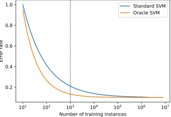
Figure 2.1: Illustrative example demonstrating the effect of convergence rate on classifier performance. Both classifiers ultimately converge on an optimal solution, but the oracle SVM does so faster. Therefore, for a given amount of training data insufficient for
op-timality, the Oracle SVM outperforms the standard SVM. For example, at 103 training
examples, marked by dashed line, the faster rate of convergence means that the Oracle SVM has error rate 0.14, whereas standard SVM has error rate 0.22.
(x1,x∗1, y1)),... , (xn,x∗n, yn), xi ∈ X, xi∗ ∈ X∗, yi ∈ −1,+1
x∗i is the privileged information that is available at training time only, generated by an
unknown probability functionP(x∗i|xi); the test data on which the model will be deployed
still consists of (xi, yi) pairs. Note that just as vectorx in spaceX is mapped to vector z
in space Z, the privileged vectorx∗ inX∗ can be mapped to vectorz∗ in space Z∗.
The privileged information is only available at training time, so the model cannot be directly fitted to these features — for example, by concatenating the normal and privileged feature vectors and providing this as input to a standard SVM — because they will not be available at deployment time. The use of this data to estimate the slacks is therefore an appealing method to use the privileged data to inform a model which is still learned in the normal feature space.
The process of learning by the SVM+ can be described as follows: two sets of weights and biases are simultaneously learned; one in the privileged space and one in the primary
feature space. The standard space weight vector and bias are denoted as w and b, as
before, and continue to define a decision boundary in the standard feature space. The
new parameters, denoted w∗ and b∗, operate in the privileged feature space and also
define a hyperplane, but this is not a decision function. Rather, it is used to inform the slack variables in the standard feature space, thereby transferring information from the privileged space. The SVM+ algorithm consists of learning these parameters through the following optimisation: R(w,w∗, b, b∗) =1 2[||w|| 2+γ||w∗||2] +C N X i=1 ξi where ξi = [hw∗,z∗ii+b∗] subject to constraints : yi[(hw,zii+b)≥1−[hw∗z∗ii+b∗] ∀i= 1...N and (hw,zii+b)≥0 ∀i= 1...N (2.12)
The equivalent Lagrangian form then is :
L(w, b, w∗, α, β) =1 2||w|| 2+γ||w∗||2+C N X i=1 [hw∗,z∗ii+b∗] − N X i=1 αi[yihw,zii+b]−1 + [hw∗,z∗ii+b ∗ ]] − N X i=1 βi[hw∗,zi∗i+b∗] (2.13)
0.0
0.5
1.0
0.25
0.00
0.25
0.50
0.75
1.00
1.25
Primary feature space
0.0
0.5
1.0
0.2
0.0
0.2
0.4
0.6
0.8
1.0
Privileged feature space
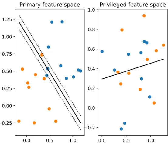
Figure 2.2: Illustrative example of the SVM+ LUPI classifer+, with two separate two-dimensional feature spaces: primary feature space (left) and privileged feature space (right). Each training data point is represented in both spaces. The decision boundary (solid line) is learned in the primary space and attempts to separate the classes, enforcing margins (dashed lines). Learning in the privileged space involves fitting a regression to the data, without taking labels into account. Information is transferred between spaces: distance from the hyperplane in the privileged space is used to inform the margin violation allowed in the primary space.
Similar to the standard SVM, this is solved by minimising with respect to w, b,w∗, b∗
and maximising with respect to the Lagrange multipliersα and β. As in standard SVM,
there is minimisation of the norm of the weight vector w, and C is a weighting
hyper-parameter to trade off minimising weights vs minimising training error. The first term of
Equation2.12shows how the newγ parameter ‘trades off’ the relative contribution of the
two weight vectors to the objective function; higher values of γ penalise the large values
in the privileged weight vector more heavily, while lower values place more emphasis on minimising the standard weight vector. Note that if one feature space in LUPI is of much
greater dimensionality, and so the norm of its weight vector is much larger, then γ may
balance the contributions of the two vectors by downweighting it.
The final term of the objective function Equation 2.12 effectively shows a regression
in the privileged space. The weights and bias in the privileged space, w∗ and b∗, define
a hyperplane, and the minimisation of this term is equivalent to fitting the hyperplane to the privileged features of all training data — of both classes. This minimisation of
the distances to the hyperplane replaces the final term in the original SVM Equation2.7,
which directly minimised the slacks (ξ1. . . ξn).
The distances therefore effectively serve as a data-dependent constraint, enforced in
the second constraint of Equation 2.12. This error upper bound is looser for data points
which have larger distances to the plane in the privileged space, so the minimisation is less concerned with correctly classifying these points. This is equivalent to providing these points with a larger, privileged data-dependent slack. In this manner, information about the dataset is transferred between feature spaces, and the privileged information is able to inform the learning of the decision boundary in the primary feature space.
Note that the data labels are not taken into account in the privileged space; all data is included in the same regression. The size of the slack in the primary space depends on the extent to which that data point is an outlier in the privileged space. Intuitively, we can take this to mean that a data point which is atypical in the privileged space can be expected to behave similarly in the primary feature space. This data point is assumed to behave in a manner which is not representative of the underlying distribution, and therefore it is difficult to predict class membership for it. Therefore, the learner should place less importance on fitting the decision boundary to correctly classify this instance. In terms of the teacher/student analogy, the privileged data is used to ‘teach’ the learner in the primary feature space which data points are outliers and which are more typical, thereby allowing the ‘student’ to focus its efforts of classification on the more typical data,
which may result in a better, more generalisable function.
Note on hyperparameters
Like the SVM, training the SVM+ requires a quadratic optimisation problem to be solved,
with similar constraints (Vapnik and Vashist,2009). However, tuning the increased
num-ber of hyperparameters for the SVM+ adds an additional computational overhead to training — for example, by performing grid-search over a larger combination of
hyper-parameters. In addition to the new trade-off parameter γ, any kernel parameters in the
privileged space also need to be selected — for example, if an RBF kernel is used inX∗,
the σ∗ parameter must be set. However, this hyperparameter optimisation is performed
at training time only, so deployment cost remains the same as standard SVM.
2.1.7 dSVM+
The dSVM+ is another SVM-based LUPI algorithm, proposed by Vapnik and Vashist
(2009) alongside the SVM+5. The two approaches are algorithmically similar, with the
dSVM+ differentiated by an additional transformative preprocessing step carried out on
the privileged data. A key point of difference is that this additional step takes the labels of training data into account in the privileged space.
Rather than learning the ‘correcting function’ in the multi-dimensional X∗ space, the
dSVM+ correcting function is defined in a one-dimensional ‘d-space’ which is constructed
for the purpose, as folllows. Firstly, a classifier is trained in X∗, to establish a decision
boundary in this privileged space. The slack variables di in this space (referred to as
‘deviation values’) for each training data point are then used as secondary input to the SVM+, in place of using the entire privileged set. In doing so, the algorithm directly “stresses the main goal [of LUPI], to provide information about the slack variables in the
simplest form” (Vapnik and Vashist,2009).
Formally, the first step of the dSVM+ is to learn ‘deviation values’ di for each xi by
finding the minimisation of the following:
5
The SVM+ in this thesis is sometimes referred to as X∗SVM+ by Vapnik and Vashist (2009) to disambiguate it fromdSVM+. For brevity and consistency, the terminology SVM+ without specification refers to SVM+ which takes the privileged feature set directly as input to the correcting function
R(w∗, b∗, ξ∗) =1 2||w ∗||2+C N X i=1 ξ∗i
subject to the constraints: yi[hw∗,xi∗i+b∗]≥1−ξ∗i ∀i∈ {1...n}
and ξi∗≥0 ∀i∈ {1...n}
(2.14)
These deviation values are then used to supplement the training data, forming triplets
(x1, d1, y1)...(xN, dN, yN) where di= 1−yi[hw∗l,x ∗ ii+b ∗ l] (2.15)
where wl and bl are the solution to equation 2.14. 3 The SVM+ described in 2.12
is then trained using these triplets, with the one-dimensional d-value for each data point
used as privileged information, instead of the original X∗ feature set itself. The authors
note that this outperforms the previous ‘X∗SVM+’ method in most experimentation.
2.1.8 SVM∆+
The SVM∆+ is an alternative LUPI classifier that is also based on the SVM (Vapnik and
Izmailov,2015). LikedSVM+, this algorithm also differs from SVM+ by taking labels into account in the privileged space. Whereas SVM+ performs a regression on the privileged
features in spaceZ∗, SVM∆+ learns a dividing hyperplane between the two classes inZ∗.
This is similar to the process of learning a classifier, but the hyperplane is not used directly as a decision boundary; the test data is not represented in this secondary feature space so there is no need to learn a generalisable decision function here. Furthermore, the boundary that is learned in the privileged space is not a max-margin classifier like the SVM. Instead, the class boundary in the privileged space is used to learn a new non-negative parameter
ζi for each data point x∗i.
It would be desirable to use the function in the privileged space as an upper bound to constrain the loss function in the standard feature space; that is: minimise
R(w, b,w∗, b∗) =1 2(||w|| 2+γ||w∗||2) +C N X i=1 [yi(hw∗z∗ii+b∗)]+ subject to: yi[hw,zii+b]≥1−[yi(hw∗,z∗ii −b ∗ )]+ where [u]+=max{0, u} (2.16)
The use of this ‘positive part’ function in the final term of the objective function
the privileged space, and no penalisation for correctly classified points. Its usage in the
constraint replaces the slack variable ξi seen in the original SVM objective function 2.7
and effectively transfers the slack from the privileged space. For datapoints zc which are
correctly classified inZ, the first constraint is fulfilled, asyi[(w,zc) +b]≥1 in these cases;
therefore the privileged data for these points does not impact the learning in the normal space and these privileged datapoints are essentially disregarded. However, for those data
pointszmwhich are misclassified inZ,yi[(w,zm)+b]<1 so the slack replacement, learned
from privileged data as the distance to the boundary inZ∗, comes into play. In short, the
slack in Z is captured by the distance to the boundary in Z∗ but only for those points
which are on the correct side of the boundary.
However, the usages of this ‘positive part’ function means that the optimisation is
non-linear. Learning the SVM∆+ therefore consists of the following approximation of
Equation 2.16, requiring the minimisation of the following:
R(w, b,w∗, b∗) =1 2(||w|| 2+γ||w∗||2) +C N X i=1 [yi(hw∗,z∗ii+b ∗ ) +ζi] + ∆C N X i=1 ζi Subject to: yi(hw,zii+b)≥1−yi(hw∗,z∗ii+b∗))−ζi and yi(hw∗,zi∗i+b∗) +ζi≥0 and ζi ≥0 (2.17)
As seen in SVM+, the norms of the weight vectors in both spaces are minimised, with
γ controlling the trade-off between the two. The ζi parameter can be thought of as a
‘privileged slack’, which ultimately impacts the decision boundary in the primary feature
space. In the standard SVM, a non-margin violating point inZ would normally have little
to no effect on the final decision boundary, as it would not be a support vector. However,
a correctly classified point in Z, that is on the wrong side of the class boundary in Z∗,
can have a big effect on the the class boundary in Z∗, which in turn affects the decision
boundary in Z. This effect is mediated by the ζi parameter.
The ζi in the second constraint of Equation 2.17, serves a similar function to ξ in
Equation 2.7, permitting boundary violations to occur when the weights and bias in the
privileged space are learned. But unlike ξ, this constraint does not enforce margins in
the privileged space, which are not required as a max-margin classifier is not learned in this space; given that these privileged parameters are learned only to inform the decision boundary in the privileged space, and the hyperplane in privileged space is not used for classification, there is no need for margins. However, the boundary is used to allow the
distance to margin to be measured. Like the standard SVM slack, ζ is minimised in the final term of the objective function. This is weighted by the product of C and ∆: a hyperparameter introduced in this formulation, and referred to as the parameter of approximation.
The SVM∆+ formulation is intuitively appealing for classification. Whereas SVM+
does not take labels into account when learning in the privileged space, the SVM∆+ does.
This means that the amount of error permitted for a given instance in the primary feature space depends on how much error it required in the privileged space. Another way to put this is that the slack depends on how much of an outlier it is in its class in the privileged space, rather than how much of an outlier it is compared to the whole dataset.
In order to incorporate the constraints and solve this quadratic optimisation problem, a Lagrangian is constructed: L(w, b,w∗, b∗,v, α, β) =1 2||w|| 2+γ||w∗||2+C N X i=1 [yi(hw∗,zi∗i+b∗) + (1 + ∆)ζi] − N X i=1 viζi− N X i=1 αi[yihw,zii+b]−1 + [yi(hw∗,z∗ii+b ∗ ) +ζi]] − N X i=1 βi[yi(hw∗,z∗ii+b∗) +ζi] (2.18)
where αi ≥0, βi≥0vi≥0, i= 1, . . . , N are Lagrange multipliers.
2.1.9 Margin Transfer
Margin Transfer is an alternative maximum-margin model for LUPI, proposed by
Shar-manska et al.(2014). In this model, an ordinary SVM is trained on the privileged dataX∗,
producing to learn privileged weightsw∗ and biasb∗. These learned parameters are then
used to calculate the distance ρi for each samplexi to the decision boundary hyperplane:
ρi :=yihw∗,x∗ii+b
∗ (2.19)
A second SVM is then trained on the original data X to produce a hyperplane with a
“data-dependent margin”. That is, for each examplexi, the margin is equal toρi, thereby
transferring information from the privileged space; this is formulated in the constraints of the following optimisation problem, the minimisation of:
R(w, b, ξ) =1 2kwk 2+C N X i=1 ξi subject to yi(hw,xii+b)≥ρi−ξi and ξi ≥0, 1≤i≤n (2.20)
It is apparent that “hard-to-classify” examples, which have small or negativeρi values,
contribute little to the optimization function; the inequality yi((w,xi) +b) ≥ ρi −ξi is
easily fulfilled due to the low ρi, so these examples are essentially ignored when setting
the decision boundary. Conversely, the “easy-to-classify” cases have higherρi, making the
inequality more difficult to satisfy. In short, the decision boundary is set in a manner which only pays attention to easily classifiable examples, and this information is obtained from the privileged domain.
This optimisation problem can be solved using standard SVM packages after
repara-meterisation. Firstly, the constraints are divided by ρi : ˆxi = ρxii and ˆξi = ρξii.The
minim-isation problem is then expressed:
R(w, b,ξˆ) =1 2kwk 2+C N X i=1 ρiξˆi subject to yi(hw,ˆxi) +bi ≥1−ξˆi and ξi ≥0, 1≤i≤n (2.21)
Margin Transfer therefore transfers information from X∗ toX about the ease of
clas-sification for each example, as does SVM+. However, Margin Transfer explicitly uses
classifier performance in X∗ to guide training in X, while SVM+ does not.
Margin Transfer has shown “comparable” performance to SVM+ in a series of image classification experiments. When the privileged feature set consisted of high-level image attributes, Margin Transfer utilised privileged information better than SVM+, leading to a greater improvement over baseline SVM score. However, when the privileged information consisted of extra image data, the greater improvement was achieved using SVM+. The authors suggest that this may be because SVM+ is more suitable when the original and privileged domains are the same. For the purposes of Learning using Unselected Features then, it can be expected that SVM+ is a more appropriate algorithm to handle two feature subsets which are not only the same domain, but from the same original dataset. Given
this lesser suitability, and the fact that this is similar to Vapnik and Izmailov (2015)’s
2.1.10 Beyond supervised learning: GPC+
Work by Hern´andez-Lobato et al. (2014) expanded LUPI beyond the SVM-based
classi-fier, building on the Gaussian Process Classifier (GPC) to produce the GPC+. This is the first Bayesian treatment of privileged information for classification, in contrast with the non-probabilistic SVM-based model seen thus far. The GPC+ uses the privileged inform-ation to model the confidence that the classifier has about a particular training example. Examples which are deemed ‘easier’ based on the representation in priviliged space cause a faster-increasing probit, while more difficult examples have a slower-increasing probit. The model for classification with ‘privileged noise’ is as follows:
Likelihood model :P r(yn= 1|xn,f˜) =I[ ˜f(xn)≥0], wherexn∈Rd
Assume : ˜f = (xn) =f(xn) +n
Privileged noise model : n∼ N(n|0, z(x∗n) =exp(g(x
∗
n))),wherex
∗ n∈Rd
∗
GP prior model :f(xn∼ GP(0, kf(xn,)) and g(x∗n)∼ GP(0, kg(x∗n,·))
(2.22)
The assumption in the second line reflects the standard assumption in a GPC that there
is some noise term n added to the noise-free latent function. However, in this classifier
which harnesses the priviliged information, the noise term n now has a different variance
z(x∗n) for each training data point, which is drawn from a distribution that depends on
the privileged information for that datapoint. GPC+ was shown to outperform standard GPC
Further work by the same authors (Sharmanska et al.,2016) expands on this Bayesian
treatment of privileged information by introducing a further learning algorithm: GPCconf.
This takes a novel approach of allowing uncertainty in the labelling of the dataset to be modelled. In the experimentation in this paper, this uncertainty was represented in terms of the disagreement between annotators that had labelled an image dataset with whether or not a given attribute appeared in the images. The level of uncertainty was supplied as privileged information, and incorporating this allowed a boost in performance relative to the standard GPC approach in a majority of datasets.
2.1.11 Beyond classification: unsupervised LUPI
Feyereisl and Aickelin (2012) describe the first usage of privileged information in the
unsupervised task of clustering, by introducing the P-dot algorithm, as follows. Firstly,
in the standard space, and separately on the privileged space. This is repeated for i
iterations with random initialisations, producingi clusterings. The clustering in standard
space which has the highest mutual information with privileged space is selected, as it is assumed to be the most reliable. For each datapoint where there is disagreement between the labels assigned in the standard and the privileged space, a measure of reliability is calculated in both spaces: the ratio between the distance of the point to the assigned centre, and to the next-closest centre. If this confidence value is higher in the privileged than in the normal space, then the privileged cluster assignment is used instead. According to this new labelling, additional attributes are added to the dataset, with values depending on the new labels. Finally, clustering is applied to this new dataset, to produce the final solution for this method.
2.1.12 Assessing SVM+ performance
Vapnik and Vashist (2009) provide proof-of-concept results alongside their introduction
to LUPI, comparing SVM+ anddSVM+ performance to that of standard SVM, in three
different problem domains. The first set of problems was composed of 80 binary protein classification problems, that required the classifier to assign a label to data, indicating its
protein superfamily. Primary feature setXconsisted of similarity measures between amino
acid sequences, and privileged feature setX∗ consisted of similarity measures between 3D
protein structures. Both implementations of LUPI outperformed standard SVM; SVM+ achieved the same accuracy in 18 cases, and lower error in the remaining 62 cases, while
dSVM+ performed equally in 14 cases and better in 66. Comparing the two LUPI
ap-proaches directly,dSVM+ performed better in 36 cases, while SVM+ was better in just 6
cases; the remaining 38 cases were tied.
Similar results were also reported for the second problem domain: a simulated
financial-forecasting task. Here, the classifiers predicted whether future steps (t+T) would be higher
or lower than current steptin a Mackey-Glass time series model (Mukherjee et al.,1997).
Here X consisted of values up to point t, and X∗ contained ‘future’ information beyond
point t (which of course would not be possible to access at model deployment time in
a real-life financial forecasting task; thereby showing a use case for LUPI). Across all
12 different settings, dSVM+ achieved equal or lower error than SVM+, which in turn
achieved lower error than standard SVM in all cases.
The final problem domain consisted of handwritten digit classification, and
in 100-dimensional pixel space, andX∗ was composed of 21-dimensional vectors based on a ‘poetic’ description of each image, with each dimension measuring an attribute of the image such as ‘stability’ or ‘tilting to the right’. Across all 6 different sizes of training datasets (40-90 instances), SVM+ achieved consistently lower error than SVM, and error
by dSVM+ was lower still.
Work byShiao and Cherkassky(2013) utilised SVM+ as an approach to handle
‘right-censored’ data in survival forecasting. In this partially incomplete setting, it is known that survival time for some individuals exceeds a certain value, but it is not known by how much. SVM+ with RBF kernel was used to predict survival at a given point as a binary classification, with this partially-unavailable data being supplied as privileged information for training instances. SVM+ accuracy was assessed across four different datasets, along with a novel ‘pSVM’ that deals with the unavailable data by allowing the notion of uncertainty in class labels. These SVM-based methods were compared with a non-SVM-based baseline: the Cox method, which is an established approach for survival-curve estimation. The SVM-based methods were more accurate in 3 of 4 datasets, with the authors noting their superiority when the survival time does not abide by classical probabilistic methods,or when there is a lot of absent information. In all cases, SVM+ accuracy score was between that of pSVM with a linear kernel, and pSVM with an RBF kernel.
LUPI has also been used to enhance performance in the domain of financial data (Ribeiro et al., 2010). SVM+ with an RBF kernel used to predict whether or not a company undergoes bankruptcy or financial distress. Standard and privileged data were taken from the ‘DIANA’ database, which describes attributes of French companies. The SVM+ approach outperformed standard SVM, and a multi-task learning approach, in terms of accuracy and F1-score.
2.1.13 Questioning the mechanism of LUPI
Recent work by Serra-Toro et al. (2014) suggests that the SVM+ can improve
perform-ance over standard SVMeven if the privileged information is randomly generated and not
meaningful. Two such conditions — one with linearly separable random features, the other non-separable — were compared with SVM+ performance using genuine privileged information, and with a standard SVM. In a handwritten digit-classification task, all three
settings produced significant improvement (p <0.05) over standard SVM, across a range
better than the non-separable random data in one setting, and the improvements by the LUPI settings were consistent even when size of validation set was altered.
However, if the s