Automatic Image Annotation Based on Particle Swarm Optimization and Support Vector Clustering

(1)

Research Article

Automatic Image Annotation Based on Particle Swarm

Optimization and Support Vector Clustering

Zhangang Hao,

1

Hongwei Ge,

2

and Tianpeng Gu

2

1_{School of Business Administration, Shandong Technology and Business University, Yantai, Shandong, China} 2_{School of Computer Science and Technology, Dalian University of Technology, Dalian Liaoning, China}

Correspondence should be addressed to Zhangang Hao; [email protected]

Received 19 December 2016; Revised 15 March 2017; Accepted 11 April 2017; Published 18 May 2017

Academic Editor: Hung-Yuan Chung

Copyright © 2017 Zhangang Hao et al. This is an open access article distributed under the Creative Commons Attribution License, which permits unrestricted use, distribution, and reproduction in any medium, provided the original work is properly cited. With the progress of network technology, there are more and more digital images of the internet. But most images are not semantically marked, which makes it difficult to retrieve and use. In this paper, a new algorithm is proposed to automatically annotate images based on particle swarm optimization (PSO) and support vector clustering (SVC). The algorithm includes two stages: firstly, PSO algorithm is used to optimize SVC; secondly, the trained SVC algorithm is used to annotate the image automatically. In the experiment, three datasets are used to evaluate the algorithm, and the results show the effectiveness of the algorithm.

1. Introduction

With the popularization of digital cameras and other digital devices, the number of images of the network has increased exponentially [1], and image retrieval technology has become a hot research topic. According to the different retrieval methods, image retrieval technology can be divided into two categories: text-based image retrieval (TBIR); content-based image retrieval (CBIR) [2–4]. The advantage of TBIR is convenient, and users can query and get the relevant results by searching the relevant keywords. However it requires manual annotation of images, the workload is very massive. CBIR searches similar images based on the visual characteristics of images. Although there are many works about CBIR [5–10], the semantic gap still exists because the images are annotated based on their low-level features such as color and texture. Many studies combine semantic infor-mation to improve content-based image retrieval techniques, and semantic information is usually composed of textual keywords that describe the semantic attributes of images. Because manually annotating semantic information is a very time-consuming and laborious work, automatic image annotation has become an increasingly crucial problem in image retrieval [11–19].

Because of the semantic gap, a gap between the low-level visual features such as colors and textures and the high-level concept which are usually used by the user in searching process, the accuracy of CBIR is not adequate. This paper presents a novel automatic image annotation algorithm (namely PSVC) based on particle swarm optimization (PSO) and support vector clustering (SVC). Instead of SMO, PSO is used to optimize SVC in PSVC, which can get support vectors without setting the parameters’ value. Comparing with SMO, PSO can get less and better support vectors. SVC is used to model the data uniformly, so as to describe the image cluster containing the same semantics with the unified model. The problem of the semantic gap is further solved by different models describing the image clusters with different semantics. Experiment results show the effectiveness of the algorithm.

2. Related Work

This work is related to use the support vector machine in automatic annotation images and some related works are reviewed for this section.

Cusano et al. [20] annotated images using SVM. All the images are handled through taking for every pixel a constant

(2)

number of partially overlapping image subdivisions which include it. Then, each of them is classified by a multi-class SVM. Each pixel is assigned to one of the categories using the results.

A confidence-based dynamic ensemble which was based on SVM was proposed to multiclass image annotation [21].

Under Multiple-Instance Learning (MIL) framework, image annotation was formulated as a supervised problem [22]. Yang et al. proposed a new algorithm, ASVM-MIL (Asymmetrical Support Vector Machine-based MIL). For false positive and false negative examples, they introduced asymmetrical loss functions to extend the conventional SVM to MIL setting.

For automatic image annotation, Qi and Han [18] inte-grated two sets of SVM, namely the MIL-based and global-feature-based SVM. The MIL-based bag features can be got through employing MIL on the image blocks, where a faster searching algorithm and enhanced diversity density algo-rithm are used to improve the accuracy and the efficiency. The results are further input to a set of SVM to find the optimum hyperplanes for annotating training images. Homogeneously, color features and global texture are input another set of SVM to categorize training images. For each test image, there are two sets of image features and they are respectively input to the two sets of SVM. Through an automatic weight estimation algorithm, the outputs are incorporated and images can be annotated by the final results.

Verma and Jawahar [23] proposed an SVM-VT (SVM with Variable Tolerance) model to annotate images. An automatically determined tolerance-parameter is introduced to the SVM-VT model, which make the SVM-VT model more tolerant of the mistakes which maybe happen in annotating images.

Based on a generative model, DMBRM (Discrete Multiple Bernoulli Relevance Model) and a discriminative model SVM, Murthy et al. [1] proposed a hybrid model for anno-tating the image. The DMBRM model is used to solve the issue of data imbalance and the SVM is used to solve the poor annotation issue.

Sahbi [24] proposed an image annotation algorithm which is based on training SVM using a class of kernels which are designed through minimizing objective functions com-bining visual features and contextual cues from surrounding tags.

Gao et al. [25] presented an automatic image annotation algorithm by incorporating feature hierarchy and boosting to scale up SVM image classifiers which are trained in dimensional feature space. The visual features which are high-dimensional, multi-modal and heterogeneous are partitioned into multiple low-dimensional single-modal homogeneous feature subsets. Each of them characterizes certain visual property of images.

Sahbi and Li [26] proposed a new image annotation method which was based on SVM and a novel class of kernels. The kernels get better values when both share the same context and the same visual content.

Using both the related semantic concepts and the prevail-ing image components, Fan et al. [27] presented an image annotation method. The salient objects are used to represent

the images’ content. For detecting the salient objects automat-ically, the SVM classifier is used to learn detection functions. For getting the semantic concepts, finite mixture models are employed to approximate the class distributions of the related salient objects. The method parameters and optimal model structure are synchronously determined by an EM algorithm. For scalable image annotation, Alham et al. [28] proposed a resource aware parallel multiclass SVM algorithm (named RAMSMO) which divided the training dataset into smaller binary chunks. A cluster of computers in parallel is used to optimize support vector machines’ training.

Although there are some works about automatic image annotation with SVM, there are few works about automatic image annotation with SVC. Because of the semantic gap, the accuracy of the automatic image recognition is not high. Therefore, the PSVC algorithm is proposed to improve the accuracy of automatic image marking.

3. Automatic Image Annotation

Based on PSVC

Firstly, the training process of SVC for multi-class is intro-duced. Secondly, PSO is used to optimize SVC. Thirdly, the trained SVC is used to annotate images automatically.

3.1. Training Process of Support Vector Clustering for

Multi-Class. Support vector clustering can be divided into single

class support vector clustering and multi-class support vector clustering. Single support vector clustering can classify data samples into two categories, but most of them are multi-class problems. A multi-class support vector clustering is needed to

solve the related problems. Assuming𝑛classes, it is necessary

to create𝑛support vector machines, which allow one of the

classes to be separated from the rest of the𝑛−1classes, where

the class is “𝑦 = 1” and the rest classes are “𝑦 = −1”, and so

on. Voting to the resulting sample and the highest score is marked as a cluster.

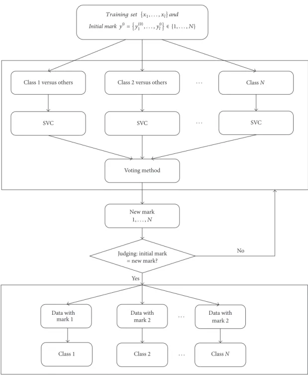
The training process of SVC for multi-class is as follows: (Figure 1):

(1) Initial training data:{𝑥₁, . . . , 𝑥_𝑙} ⊆ 𝑋; initial mark:

𝑦0= {𝑦₁(0), . . . , 𝑦_𝑙0} ∈ {1, . . . , 𝑁};

(2) Using{𝑥₁, . . . , 𝑥_𝑙} ⊆ 𝑋 and 𝑦0 = {𝑦₁(0), . . . , 𝑦_𝑙0} ∈

{1, . . . , 𝑁} to train support vector clustering and

getting𝑦𝑡 = {𝑦₁(𝑡), . . . , 𝑦_𝑙𝑡} ∈ {1, . . . , 𝑁}; if𝑦𝑡 = 𝑦0,

terminating the iteration, otherwise to (3);

(3) Using{𝑥₁, . . . , 𝑥_𝑙} ⊆ 𝑋and𝑦𝑡 = {𝑦₁(𝑡), . . . , 𝑦_𝑙𝑡} ∈ {1,

. . . , 𝑁}to train support vector clustering and getting

𝑦𝑡+1_{= {𝑦}(𝑡+1)

1 , . . . , 𝑦𝑙𝑡+1} ∈ {1, . . . , 𝑁};

(4) If𝑦𝑡+1 = 𝑦𝑡, terminating the iteration, otherwise𝑡 =

𝑡 + 1,𝑦𝑡= 𝑦𝑡+1, to (3).

The training process is relatively simple and the conver-gence speed is faster. In the training process of SVC, the tag allocation does not appear in the clustering algorithm, so the training time is significantly reduced.

(3)

Class 1 versus others Class 2 versus others Class _N SVC SVC SVC Voting method New mark No Yes Data with mark 1 Data with mark 2 Data with mark 2

Class 1 Class 2 Class _N

Judging: initial mark = new mark? · · · · · · · · · · · · 1, . . . , N

Training set {x1, . . . , xl}and {y₁(0), . . . , y_l0} {1, . . . , N}

y0= ∈

Initial mark

Figure 1: Training process of support vector clustering for multi-class.

3.2. Optimizing SVC Based on PSO. The most common

method of training support vector clustering is the sequential minimal optimization (SMO) [29] to get the Lagrangian

multiplier. The parameter combination{𝐶, 𝜉}plays a decisive

role, where𝐶is the penalty parameter and𝜉is the relaxation

factor. The value of the penalty parameter𝐶directly affects

the experience error and the complexity of the learning

ability. The relaxation factor𝜉controls the number of support

vectors in the support vector clustering so as to control the sparse points. However, the parameters are often set by

experience, which brings uncertainty to the results. Instead of SMO, PSO is used to train SVC in this paper, which can get support vectors without setting the parameters’ value.

According to the support vector clustering model, the

Lagrangian multipliers,𝛼_𝑖(𝑖 = 1, 2, . . . , 𝑙), need to be found

firstly. The adaptive function of the particle is:

min_𝛼 1 2 𝑙 ∑ 𝑖=1 𝑙 ∑ 𝑗=1𝑦𝑖𝑦𝑗𝐾 (𝑥𝑖, 𝑥𝑗) 𝛼𝑖𝛼𝑗− 𝑙 ∑ 𝑗=1𝛼𝑗 (1)

(4)

The initial position of the particle should meet the follow-ing constraints: 𝑙 ∑ 𝑖=1 𝛼_𝑖𝑦_𝑖= 0, 0 ≤ 𝛼_𝑖≤ 𝐶, 𝑖 = 1, 2, . . . , 𝑙 (2) Because of the local optimal value constraint, the effi-ciency of the PSO algorithm is reduced and the convergence speed of the particle is severely affected. In this paper, SVC is trained by dynamically changing the weight parameters to accelerate the convergence of the PSO algorithm. The main steps based on PSO to optimize SVC are as follows.

For each particle, there is a velocity information𝑉_𝑖∈ 𝑅𝑛

and location information𝑋_𝑖 ∈ 𝑅𝑛, and the total number of

particle is𝑆. Let𝑃_𝑖be the best position of the𝑖th particle, and

𝑔be the global optimal position known to the particle:

(i) Initializing all particles, for each particle,𝑖 = 1, 2, . . . ,

𝑆:

(a) Uniform random variables generate the random

number. And𝑏_lo, 𝑏_up represent the upper and

lower bounds of the search space respectively.

The initial iteration number is set to iter = 0,

and the maximum number of iterations is 1000; (b) Initializing the location information of the

par-ticle𝑃_𝑖← 𝑋_𝑖.

(c) If 𝑓(𝑃_𝑖) < 𝑓(𝑔), updating 𝑖th particle’s best

location information𝑔 ← 𝑃_𝑖;

(d) Initializing 𝑖th particle’s velocity information

𝑉𝑖∈ 𝑈(−|𝑏lo− 𝑏up|, |𝑏lo− 𝑏up|).

(ii) If Meeting the iteration number or finding the global optimal solution, stopping the calculation, otherwise repeating the following steps:

To each particle𝑖 = 1, 2, . . . , 𝑆:

(a) To each dimension𝑑 = 1, 2, . . . , 𝑛,

(1) Selecting a random number rand_𝑝, rand_𝑝∈

𝑈(0, 1);

(2) Updating particle’s velocity:𝑉_𝑖,𝑑= 𝜔∗𝑉_𝑖,𝑑+

𝑐₁∗rand_𝑝∗ (𝑃_𝑖,𝑑− 𝑋_𝑖,𝑑) + 𝑐₂∗rand_𝑔∗ (𝑔_𝑑−

𝑋_𝑖,𝑑).

(3) Determining the velocity in the bound or not.

(b) To each dimension, updating particle’s position:

𝑋_𝑖← 𝑋 + 𝑉_𝑖;

(c) If𝑓(𝑋_𝑖) < 𝑓(𝑃_𝑖),

(1) Updating particle’s best position𝑃_𝑖← 𝑋_𝑖;

(2) If𝑓(𝑃_𝑖) < 𝑓(𝑔), updating particle swarm’s

best position:𝑔 ← 𝑃_𝑖;

(iii) According to step (ii), finding the global optimization

𝑔;

(iv) The global optimal solution is the Lagrangian

multi-plier,𝛼_𝑖(𝑖 = 1, 2, . . . , 𝑙), in the support vector

cluster-ing, and then the decision function is calculated, and

all the number and value of the support vector can be obtained.

𝑓 (𝑥) =sgn(𝑔 (𝑥)) (3)

The formula𝑔(𝑥)can be expressed in the following form:

𝑔 (𝑥) = (𝑤∗⋅ 𝑥) + 𝑏∗=∑𝑙 𝑖=1

𝛼∗𝑦_𝑖𝐾 (𝑥_𝑖, 𝑥_𝑗) + 𝑏∗ (4) Particle swarm optimization algorithm is to find the optimal solution in the randomly formed particles by con-tinuous iteration. For support vector clustering in solving the problem of quadratic programming, the first difficulty is the problems of linear constraint and inequality constraint, which encounters problems such as a large amount of time-consuming and memory in the process of operation. By using the particle swarm optimization, the learning ability of support vector clustering is improved, and the trained model is used to automatic image annotation.

3.3. Process of Automatic Image Annotation

3.3.1. Extracting Images’ Features Based on CPAM. Colored

pattern appearance model (CPAM) not only can extract the visual features around the salient point, but also contains the visual features of the whole picture [30], so it is more suitable for the requirement of image semantic annotation. CPAM is used to compress the image and extract the characteristics of the image, including the visualization of color and texture. Based on these, support vector clustering related information is generated. The final probability estimation method is used to mark the given image through the support vector description model. The eigenvalues extracted by CPAM con-tain statistical color and achromatic spatial patterns, which represent colors and textures. Through CPAM, the images are

split into4 × 4 blocks, each containing achromatic spatial

pattern histograms (ASPH) and Chromatic spatial pattern histograms (CSPH). The eigenvectors of one image extracted by CPAM contain 128 eigenvalues, of which 64 are color eigenvalues and 64 are achromatic pattern eigenvalues. Thus, each image is represented by a 128-dimensional vector.

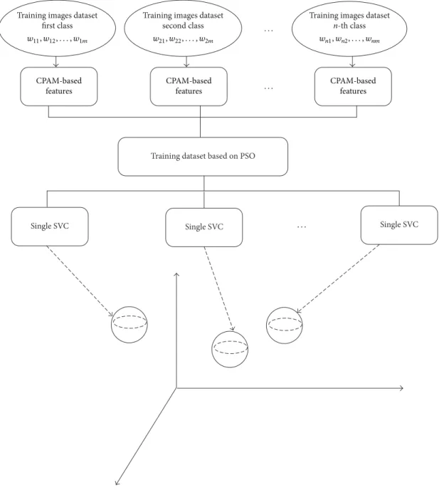
3.3.2. Training Single Support Vector Clustering. As shown in

Figure 2, a process of training support single vector

cluster-ing, the training data contains𝑛image clustering, each

clus-tering contains𝑥_𝑖 = {img_𝑖1,img_𝑖2, . . . ,img_𝑖𝑚}images. Each

clustering is manually marked with a set of semantics,𝑥_𝑖 =

{img_𝑖1,img_𝑖2, . . . ,img_𝑖𝑚}, to describe the class, where the

semantic word is a subset of all the thesaurus,𝑊 = {𝑤₁,

𝑤₂, . . . , 𝑤_𝑚},𝑤_𝑖 ⊆ 𝑊. An example of semantic word anno-tation is as Box 1.

For each training image, eigenvalues based on color features and texture features are extracted using CPAM. During the training process, these eigenvalues are mapped to the high-dimensional feature space by non-linear transfor-mation, looking for all minimum enclosing balls, and each of them is a separate class.

(5)

w11, w12, . . . , w1m Training images dataset

first class

w21, w22, . . . , w2m

Training images dataset second class

wn1, wn2, . . . , wnm

Training images dataset

n-th class CPAM-based features CPAM-based features CPAM-based features . . . . . . . . .

Training dataset based on PSO

Single SVC Single SVC Single SVC

Figure 2: The process of training single support vector clustering.

(0) Africa, people, landscape, animal (1) autumn, tree, landscape, lake

(2) Bhutan, Asia, people, landscape, church (3) California, sea, beach, ocean, flower (4) Canada, sea, boat, house, flower, ocean

(5) Canada, west, mountain, landscape, cloud, snow, lake (6) China, Asia, people, landscape, historical building (7) Croatia, people, landscape, house, church (8) death valley, landscape, cloud, mountain, lake (9) dog, animal, grass

Box 1: Semantic word annotation of each class.

3.3.3. Clustering Density Estimation. Assuming a data set{𝑥₁,

𝑥₂, . . . , 𝑥_𝑛} ∈ 𝜒, its probability distribution is𝑝. The

prox-imity value𝑝is made by using a weighted kernel probability

density estimate [31]:

̂𝑝 (𝑥) =∑𝑛

𝑗=1𝜔𝑗𝜑 (𝑥, 𝑥𝑗) , (5)

where𝜑(𝑥, 𝑥_𝑗)is a window function and0 ≤ 𝜔 ≤ 1is the

𝑗th window’s weight,∑𝑛_𝑗=1𝜔_𝑗 = 1. Without loss of generality,

Gaussian function is used:

𝜑 (𝑥_𝑖, 𝑥_𝑗) = 1

(6)

In a single support vector clustering model, the enclosing ball is satisfied in the high dimensional space by using the

trained kernel radius equation. Radius of the ball𝑅, test data

𝑥, let𝑥be outside the ball, then:

𝑓 (𝑥) = 𝐾 (𝑥, 𝑥) − 2∑𝑛 𝑗=1 𝛽_𝑗𝐾 (𝑥, 𝑥_𝑗) +∑𝑛 𝑖=1 𝑛 ∑ 𝑗=1 𝛽_𝑖𝛽_𝑗𝐾 (𝑥_𝑖, 𝑥_𝑗) > 𝑅2 (7) Because of𝐾(𝑥, 𝑥) = 1, then: 𝑛 ∑ 𝑗=1 𝛽_𝑗𝐾 (𝑥, 𝑥_𝑗) <1 2(1 + 𝑛 ∑ 𝑖=1 𝑛 ∑ 𝑗=1 𝛽_𝑖𝛽_𝑗𝐾 (𝑥_𝑖, 𝑥_𝑗) − 𝑅2) (8)

Similarly, if test data𝑥is inside or on the sphere, then:

𝑛 ∑ 𝑗=1 𝛽_𝑗𝐾 (𝑥, 𝑥_𝑗) ≥1₂(1 +∑𝑛 𝑖=1 𝑛 ∑ 𝑗=1 𝛽_𝑖𝛽_𝑗𝐾 (𝑥_𝑖, 𝑥_𝑗) − 𝑅2) (9)

According to formulas (5), (6) and∑𝑛_𝑗=1𝛽_𝑗𝐾(𝑥, 𝑥_𝑗), then:

𝑛 ∑ 𝑗=1

𝛽_𝑗𝐾 (𝑥, 𝑥_𝑗) = √2𝜋𝛿2_{∗ ̂𝑝 (𝑥)} ₍₁₀₎

The probability density follows the following formula:

𝑑 = 1 + ∑ 𝑛

𝑖=1∑𝑛𝑗=1𝛽𝑖𝛽𝑗𝐾 (𝑥𝑖, 𝑥𝑗) − 𝑅2

2√2𝜋𝛿2 (11)

So the following relationship is drawn:

(1) If the input data𝑥is outside the sphere then̂𝑝(𝑥) < 𝑑;

(2) Similarly, if the input data𝑥is located on the surface

or inside of the sphere, then̂𝑝(𝑥) ≥ 𝑑.

The trained kernel-radius function of the support vector clustering is used to achieve the distribution of the clusters by

using a probability density estimate. Given the test data𝑥, the

probability densitŷ𝑝(𝑥)gradually increases as the test data𝑥

approaches the center of the sphere.

3.3.4. Automatic Image Annotation. The automatic image

annotation system consists of a single support vector clus-tering model, which is based on feature information such as

color and texture. The support vector clustering model has𝑁

sub-models; each model has been marked with the relevant semantic word. If the test image is given, the CPAM model is used to extract the feature information of the image. Then, the probability density of the test image is calculated by a single support vector clustering model. The formula is as follows:

̂𝑝 (𝑥) = 1 √2𝜋𝛿2 𝑛 ∑ 𝑗=1 𝛽_𝑗𝐾 (𝑥, 𝑥_𝑗) , (12)

where 𝑥 is the test image’s eigenvalue extracted by CPAM

model. Setting the semantics,𝑤_𝑖= {𝑤_𝑖1, 𝑤_𝑖2, . . . , 𝑤_𝑖𝑚_𝑖}, which

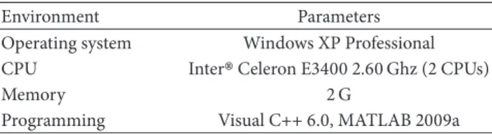
Table 1: Experiment environment.

Environment Parameters

Operating system Windows XP Professional

CPU InterCeleron E3400 2.60 Ghz (2 CPUs)

Memory 2 G

Programming Visual C++ 6.0, MATLAB 2009a

describe a class. To each𝑤_𝑖𝑘 ∈ 𝑤_𝑖, the probability of 𝑤_𝑖𝑘

establishes a correlation with the test image through the

probability density. The set of all semantic words is 𝑊 =

{𝑤₁, 𝑤₂, . . . , 𝑤_𝑚}, and calculating semantic words set 𝜉(𝑤_𝑖)

which contains the semantic word 𝑤_𝑖. Then the semantic

word containing𝜉(𝑤_𝑖)can be used to generate a probability

density value by testing the image. The formula is as follows:

𝑞 (𝑤_𝑖) = max

𝑘,𝑘∈𝜉(𝑤𝑖)̂𝑝𝑘(𝑥) (13)

Creating an𝑚-dimensional instruction vector that sets

the initial value of all support vectors to zero. Then

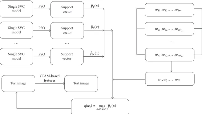
{𝑞(𝑤₁), 𝑞(𝑤₂), . . . , 𝑞(𝑤_𝑚)}are stored in descending order, and the highest instruction vector value is set to maximum. And so on, an instruction vector is created for the test image at each step. The semantic word with the maximum instruction vector value is the final decision value, and the semantic word is selected. Similarly, the same method is used for other semantic words. Setting a threshold that represents the number of annotation words for each test image, and usually the threshold is four. The process of automatic image annotation is as Figure 3.

4. Experimental Results

The experimental environment is showed in Table 1, and the programming environment is Matlab and Visual C++ 6.0. Core 160 k data set is used as experimental data, which contains 60,000 images, and the image is JPEG format,

specifications for 384 ∗ 256 or 256 ∗ 384. The data set is

divided into 600 clusters, each with 100 images, each cluster of images belonging to the same theme. Each cluster is manually marked with group descriptive words which are a description of the whole cluster, rather than a single image. The total number of words is 441, then the average number of annotations for each cluster is 3.6. In addition to the core 160 dataset, Google 6000 data sets containing 6000 images downloaded from the Internet by Google are used to test PSVC algorithms.

4.1. Feature Extraction. All 600 clusters (each cluster

contain-ing 100 images) are extracted feature uscontain-ing the CPAM method [32]. The extracted eigenvalues are saved to one file. In the file, 0 value is deleted and 0 to 599 indicates different clusters. In Box 2, The first data “1” indicates the cluster label; the second data “1:” indicates the first dimension eigenvector of an image, and the “0.0076497” after the colon indicates the specific eigenvector value, and so on.

(7)

1 1:0.0076497 2:0.0063477 3:0.0050456 4:0.0024414 5:0.0052083 8:0.00358 10:0.047852 11:0.0086263 12:0.1263 13:0.018066 14:0.0053711 15:0.014648 18:0.0076497 19:0.0048828 21:0.0047201 22:0.0037435 23:0.0030924 26:0.2 27:0.0069987 29:0.013672 30:0.004069 31:0.0084635 32:0.0032552 33:0.00 35:0.0050456 37:0.010417 38:0.0045573 39:0.0014648 40:0.025391 41:0.00 42:0.0071615 43:0.0032552 44:0.00065104 45:0.0056966 46:0.004069 47:0.2 48:0.0052083 49:0.0043945 50:0.0056966 51:0.0013021 52:0.01416 53:0.00 54:0.0024414 55:0.0052083 56:0.0079753 57:0.004069 58:0.0032552 59:0.0 61:0.0048828 62:0.0024414 63:0.012044 64:0.026693 65:0.0030924 66:0.003 67:0.00048828 69:0.0091146 70:0.0035807 71:0.0011393 72:0.00016276 73:1 74:0.0014648 75:0.0018531 77:0.0014648 78:0.014874 79:0.0050456 80:0.0

Box 2: Feature extraction using CPAM model.

SV 0.2151573429 1:0.0100910 2:0.0211590 3:0.0042318 4:0.002 0.1043309117 1:0.0029297 2:0.0017904 3:0.0052083 4:0.003 0.4296885850 1:0.0001628 2:0.0001628 3:0.0001628 4:0.000 0.0586808399 1:0.0126950 2:0.0126950 3:0.0016276 4:0.003 0.1986436216 1:0.0073242 2:0.0273440 3:0.0069029 4:0.009 Box 3: The result of training sample using PSO algorithm.

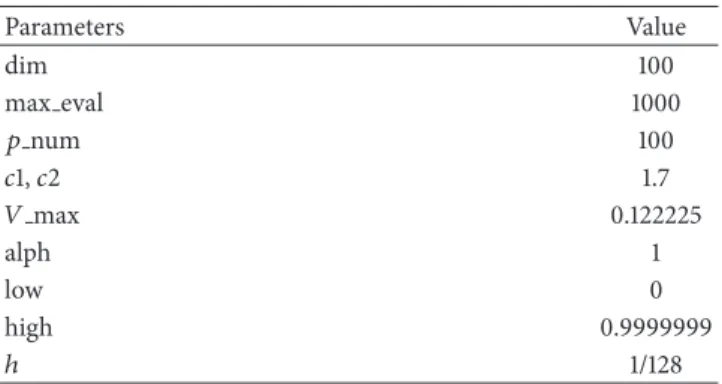
Table 2: Parameter values of PSO algorithm.

Parameters Value dim 100 max eval 1000 𝑝num 100 𝑐1,𝑐2 1.7 𝑉max 0.122225 alph 1 low 0 high 0.9999999 ℎ 1/128

4.2. Training Data Sets Using PSO Algorithm. The extracted

eigenvalues are used as inputs to the PSO algorithm, and 600 clusters are experimented repeatedly to determine the parameters. The parameter values of PSO are showed in Table 2.

Because the main factors affecting the PSO algorithm are the number of iterations, five clusters are randomly selected to reflect the relationship between the number of iterations and the convergence. As shown in Figure 4, horizontal axis is the number of iterations and vertical axis is convergence. When iteration is about 1000 times, five clusters are convergence. From Figure 4, the convergence of different cluster may be different. A cluster with fast convergence is easy to automati-cally annotate.

PSO algorithm is mainly used to get the Lagrangian multiplier in the support vector clustering training and then find the support vector. With supporting vector, the keywords of the test image are extracted by the probability calculation. The resulting Lagrangian multipliers are saved to

0.2151573429 0.1043309117 0.4296885850 0.0586808399 0.1986436216

Box 4: A file only including Lagrange multiplier. Table 3: Parameters of Libsvm software.

Parameters Value

(i)𝑠 2 (one-class)

(ii)𝑡 2 (RBF kernel function)

(iii)𝑛 0.05

coef 0∼599 files. A file via notepad is opened, as showing in

Box 3.

In Box 3, the data sample has five support vectors, and the Lagrangian multiplier is the first element of each row. A file containing only the Lagrangian multiplier is opened with a notepad, as showing in Box 4.

The Libsvm software [33] using the SMO algorithm is used to train the data to get the Lagrangian multiplier and the support vector. The Libsvm software parameters are showed in Table 3, give the remaining parameters for the default value. The results of the PSO algorithm and the SMO algorithm are showed in Table 4.

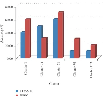
600 clusters are annotated respectively using PSVC algo-rithm and libsvm algoalgo-rithm, and randomly selected five clusters for analysis. In Figure 5, the horizontal axis represents a random five clusters, and the vertical axis represents the accuracy which means an image can be successfully marked.

(8)

Single SVC model Single SVC model Single SVC model

Test image Test image

Support vector Support vector Support vector PSO PSO PSO CPAM-based features w11, w12, . . . , w1m1 w21, w22, . . . , w2m2 wn1, wn2, . . . , wnm_n w1, w2, . . . , wN  p1(x)  p2(x)  pN(x) = Ｇ；Ｒ k,k∈(w)pk(x) q(wi) · · · ·

Figure 3: The process of automatic image annotation. Table 4: The comparison of results using PSO algorithm and SMO

algorithm.

PSO SMO

Datasets Number of

support vectors Datasets

Number of support vectors 100 5 100 7 400 11 400 27 700 34 700 47 1000 60 1000 66 1300 67 1300 88 1600 105 1600 110 1900 115 1900 128 2200 139 2200 150 2500 178 2500 170 2800 185 2800 192 3100 214 3100 213 3400 223 3400 231 3700 253 3700 255 4000 270 4000 278 5000 327 5000 354 6000 372 6000 423

From the experimental results, the effect of PSO algorithm is better than SMO algorithm for clustering of 1, 31, 45 and 133. But for the 24th cluster, the SMO algorithm is slightly better than the PSO algorithm. In general, using PSO algorithm in the automatic image annotation is better than using SMO algorithm.

Table 5: Performance comparison of four models.

𝑃 𝑅 𝐹1-Score TGLM 0.26 0.28 0.27 Group sparsity 0.29 0.33 0.31 TagProp 0.32 0.39 0.35 SVC 0.33 0.31 0.32 GPR 0.34 0.40 0.37 CS 0.31 0.38 0.34 PSVC 0.42 0.38 0.40

Table 6: Performance comparison of two extraction methods.

𝑃 𝑅 𝐹1-Score

SIFT 0.44 0.40 0.42

CPAM 0.42 0.40 0.41

4.3. Performance Comparision with Other Algorithms. The

PSVC algorithm is compared with the other algorithms using Core 160 k, including SVC using SMO, TagProp model [34], TGLM model [35], Group Sparsity model [36], GPR [33], CS [37]. Three measures “average precision” (P), “average recall”

(R) and “𝐹1-Score” are used to evaluate the algorithms and

the results are showed in Table 5.

From Table 5, it can be seen that the precision of PSVC has been greatly improved, which proves the model’s feasibility. Although the recall is lower than GPR algorithm, it has

reached a high level and the comprehensive index𝐹1-Score

is the highest in Table 5.

Using SIFT and CPAM to extract features separately, PSVC is used to annotate images of the ImageNet dataset which are popular dataset in image annotation. The results

(9)

Table 7: (a) Annotating test images. (b) Annotating test images. (c) Annotating test images. (a)

Test images

Annotation words Dog, animal, grass Ocean animal, bird, ocean,

turtle Plant, landscape, flower, ocean Painting, Europe

(b)

Test images

Annotation words lion, animal, wild life, grass Africa, people, landscape,_animal China, people, historical_building Yuletide, Christmas,_holiday (c)

Test images

Annotation words Penguin, ocean, ice, bird, sky Plant, grass, landscape,

garden, historical building People, face Work, people, cloth

C o n ve rge nc e Cluster 31 Cluster 35 Cluster 133 Cluster 24 Cluster 1 Iterations’ number 300 700 1000 1500

Figure 4: The relation between the iterations’ number and conver-gence.

are showed in Table 6. From Table 6, it can be seen that SIFT and CPAM are both effective feature extraction methods.

4.4. Annotating Google 6000 Data Sets Using PSVC. For

better evaluating our algorithm, PSVC algorithm is used to Google 6000 data sets downloaded from the Internet. As showing in Table 7, the test image is successfully marked.

Cl ust er 1 Cl ust er 24 Cl ust er 31 Cl ust er 35 Cl ust er 133 Cluster LIBSVM PSVC 0.00 20.00 40.00 60.00 80.00 A cc urac y (%)

Figure 5: The result comparison of PSVC and libsvm.

5. Conclusion and Future Work

With the progress of network technology, there are more and more digital images of the internet. To facilitate the management of these massive digital images, semantic

(10)

annotation to the image is needed. In this paper, the PSVC algorithm which combines with PSO algorithm and SVC algorithm is proposed to annotate the images automatically. At the next stage, image-based search that can be used for multiple areas based on image auto-tagging will be performed.

Conflicts of Interest

The authors declare that they have no conflicts of interest.

References

[1] V. N. Murthy, E. F. Can, and R. Manmatha, “A hybrid model for automatic image annotation,” in2014 4th ACM International Conference on Multimedia Retrieval, ICMR 2014, pp. 369–376, GBR, April 2014.

[2] N. Vasconcelos and M. Kunt, “Content-based retrieval from image databases:current solutions and future directions,” in Inprocedings of the 2001 international Conference on Image Processing, vol. 3, pp. 6–9.

[3] A. W. M. Smeulders, M. Worring, S. Santini, A. Gupta, and R. Jain, “Content-based image retrieval at the end of the early years,” IEEE Transactions on Pattern Analysis and Machine Intelligence, vol. 22, no. 12, pp. 1349–1380, 2000.

[4] R. Datta, D. Joshi, J. Li, and J. Z. Wang, “Image retrieval: ideas, influences, and trends of the new age,”ACM Computing Surveys, vol. 40, no. 2, article 5, 2008.

[5] J. Z. Wang, J. Li, and G. Wiederhold, “SIMPLIcity: semantics-sensitive integrated Matching for Picture Libraries,”IEEE Trans-actions on Pattern Analysis and Machine Intelligence, vol. 23, no. 9, pp. 947–963, 2001.

[6] K. Barnard, P. Duygulu, and D. Forsyth, “Clustering art[C],” in Inproceedings of the 2001 IEEE Computer Society Conference on Computer Vision and Pattern Recognition, pp. 434–439. [7] Y. Chen and J. Z. Wang, “A region-based fuzzy feature matching

approach to content-based image retrieval,”IEEE Transactions on Pattern Analysis and Machine Intelligence, vol. 24, no. 9, pp. 1252–1267, 2002.

[8] Q. Iqbal and J. K. Aggarwal, “Retrieval by classification of images containing large manmade objects using perceptual grouping,”Pattern Recognition, vol. 35, no. 7, pp. 1463–1479, 2002.

[9] K. Barnard, P. Duygulu, D. Forsyth, N. De Freitas, D. M. Blei, and M. I. Jordan, “Matching Words and Pictures,”Mach. Learn. Res, vol. 3, pp. 1107–1135, 2003.

[10] Q. Zhang, S. A. Goldman, and W. Yu, “Content-based image retrieval using multiple-instance learning,” inInproceedings of the 19th International Conference on Machine Learning, pp. 682– 689, 2002.

[11] D. Zhang, M. M. Islam, and G. Lu, “A review on automatic image annotation techniques,”Pattern Recognition, vol. 45, no. 1, pp. 346–362, 2012.

[12] Z. Chen, J. Hou, D. Zhang, and X. Qin, “An annotation rule extraction algorithm for image retrieval,”Pattern Recognition Letters, vol. 33, no. 10, pp. 1257–1268, 2012.

[13] Y. Wang, T. Mei, S. Gong, and X.-S. Hua, “Combining global, regional and contextual features for automatic image annota-tion,”Pattern Recognition, vol. 42, no. 2, pp. 259–266, 2009. [14] N. Yu, K. A. Hua, and H. Cheng, “A Multi-directional search

technique for image annotation propagation,”Journal of Visual

Communication and Image Representation, vol. 23, no. 1, pp. 237–244, 2012.

[15] J. Yao, Z. Zhang, S. Antani, R. Long, and G. Thoma, “Automatic medical image annotation and retrieval,”Neurocomputing, vol. 71, no. 10-12, pp. 2012–2022, 2008.

[16] Y. Gao, Y. Yin, and T. Uozumi, “A hierarchical image annotation method based on SVM and semi-supervised EM,”Acta Auto-matica Sinica, vol. 36, no. 7, pp. 960–967, 2012.

[17] R. Li, J. Lu, Y. Zhang, and T. Zhao, “Dynamic Adaboost learning with feature selection based on parallel genetic algorithm for image annotation,”Knowledge-Based Systems, vol. 23, no. 3, pp. 195–201, 2010.

[18] X. Qi and Y. Han, “Incorporating multiple SVMs for automatic image annotation,”Pattern Recognition, vol. 40, no. 2, pp. 728– 741, 2007.

[19] N. El-Bendary, T.-H. Kim, A. E. Hassanien, and M. Sami, “Auto-matic image annotation approach based on optimization of classes scores,”Computing, vol. 96, no. 5, pp. 381–402, 2014. [20] C. Cusano, G. Ciocca, and R. Schettini, “Image annotation using

svm,” inInternet Imaging V, pp. 330–338, USA, January 2004. [21] K.-S. Goh, E. Y. Chang, and B. Li, “Using one-class and two-class

SVMs for multiclass image annotation,”IEEE Transactions on Knowledge and Data Engineering, vol. 17, no. 10, pp. 1333–1346, 2005.

[22] C. Yang, M. Dong, and J. Hua, “Region-based image annotation using asymmetrical support vector machine-based multiple-instance learning,” in2006 IEEE Computer Society Conference on Computer Vision and Pattern Recognition, CVPR 2006, pp. 2057–2063, usa, June 2006.

[23] Y. Verma and C. V. Jawahar, “Exploring SVM for image annotation in presence of confusing labels,” in2013 24th British Machine Vision Conference, BMVC 2013, GBR, September 2013. [24] H. Sahbi, “CNRS-TELECOM Paris Tech at Image CLEF 2013 Scalable Concept Image Annotation Task: Winning Annota-tions with Context Dependent SVMs,” inCLEF 2013 Evaluation Labs and Workshop, Online Working Notes, pp. 23–26, 2013. [25] Y. Gao, J. Fan, H. Luo, X. Xue, and R. Jain, “Automatic image

annotation by incorporating feature hierarchy and boosting to scale up SVM classifiers,” in14th Annual ACM International Conference on Multimedia, MM 2006, pp. 901–910, USA, Octo-ber 2006.

[26] H. Sahbi and X. Li, “Context based support vector machines for interconnected image annotation,” inIn the Asian Conference on Computer Vision (ACCV), 2010.

[27] J. Fan, Y. Gao, H. Luo, and G. Xu, “Automatic image annotation by using concept-sensitive salient objects for image content representation,” in Inproceedings of the 27th Annual Interna-tional Conference on Research and Development in Information Retrieval, pp. 361–368, 2004.

[28] N. K. Alham, M. Li, and Y. Liu, “Parallelizing multiclass support vector machines for scalable image annotation,”Neural Computing and Applications, vol. 24, no. 2, pp. 367–381, 2014. [29] C. Platt J,Fast Training of Support Vector Machines Using

Se-quential Minimal Optimization, MIT Press, 1999.

[30] N. Zhou, W. K. Cheung, G. Qiu, and X. Xue, “A hybrid proba-bilistic model for unified collaborative and content-based image tagging,”IEEE Transactions on Pattern Analysis and Machine Intelligence, vol. 33, no. 7, pp. 1281–1294, 2011.

[31] P. Hall and A. Turlach B, “Reducing bias in curve estimation by use of weights,”Computational Statistics & Data Analysis, vol. 30, no. 1, pp. 67–86, 1999.

(11)

[32] A. Abdiansah and R. Wardoyo, “Time complexity analysis of Support Vector Machines (SVM) in LibSVM,” International Journal of Computer Applications, vol. 128, no. 3, pp. 975–8887, 2015.

[33] L. Denoyer and P. Gallinari, “A Ranking based model for auto-matic image annotation in a social network,” inInproceedings of the Fourth International AAAI Conference on Weblogs and Social, pp. 231–234, 2016.

[34] M. Guillaumin, T. Mensink, J. Verbeek, and C. Schmid, “Tag-Prop: discriminative metric learning in nearest neighbor mod-els for image auto-annotation,” inProceedings of the IEEE 12th International Conference on Computer Vision (ICCV ’09), pp. 309–316, IEEE, Kyoto, Japan, September-October 2009. [35] J. Liu, M. Li, Q. Liu, H. Lu, and S. Ma, “Image annotation via

graph learning,”Pattern Recognition, vol. 42, no. 2, pp. 218–228, 2009.

[36] S. Zhang, J. Huang, Y. Huang, Y. Yu, H. Li, and D. N. Metaxas, “Automatic image annotation using group sparsity,” in 2010 IEEE Computer Society Conference on Computer Vision and Pattern Recognition, CVPR 2010, pp. 3312–3319, USA, June 2010. [37] S. Kharkate K and J. Janwe P N, “A novel approach for automatic image annotation using color saliency,”International Journal of Innovative Research in Computer & Communication Engineer-ing, vol. 1, no. 5, pp. 1142–1148, 2013.

(12)

Submit your manuscripts at

https://www.hindawi.com

Hindawi Publishing Corporation

http://www.hindawi.com Volume 2014

Mathematics

Journal of

Mathematical Problems in Engineering

Hindawi Publishing Corporation http://www.hindawi.com

Differential Equations

International Journal of

Volume 2014

http://www.hindawi.com Volume 2014 Hindawi Publishing Corporationhttp://www.hindawi.com Volume 2014

http://www.hindawi.com Volume 2014 Mathematical PhysicsAdvances in

Complex Analysis

Journal of

Optimization

Journal of

Combinatorics

http://www.hindawi.com Volume 2014 International Journal of

Journal of Hindawi Publishing Corporation

Function Spaces

Abstract and Applied Analysis

http://www.hindawi.com Volume 2014 International Journal of Mathematics and Mathematical Sciences

Hindawi Publishing Corporation http://www.hindawi.com Volume 201

The Scientific

World Journal

Discrete Dynamics in Nature and Society Hindawi Publishing Corporation

#HRBQDSDĮ,@SGDL@SHBR

Journal of

http://www.hindawi.com Volume 2014 Hindawi Publishing Corporationhttp://www.hindawi.com Volume 2014

Automatic Image Annotation Based on Particle Swarm Optimization and Support Vector Clustering

Research Article