Liu, X., Zhang, Z. and J. Peterson (2009). Evaluation of the performance of DEM interpolation algorithms for LiDAR data. In: Ostendorf, B., Baldock, P., Bruce, D., Burdett, M. and P. Corcoran (eds.), Proceedings of the Surveying & Spatial Sciences Institute Biennial International Conference, Adelaide 2009, Surveying & Spatial Sciences Institute, pp. 771-780. ISBN: 978-0-9581366-8-6.
EVALUATION OF THE PERFORMANCE OF DEM
INTERPOLATION ALGORITHMS FOR LIDAR DATA
Xiaoye Liu1, 2, Zhenyu Zhang1, 2, Jim Peterson2
1
Faculty of Engineering and Surveying
University of Southern Queensland, Toowoomba, Queensland 4350, Australia
2
Centre for GIS, School of Geography and Environmental Science Monash University, Clayton, Victoria 3800, Australia
Email: [email protected] [email protected] [email protected]
ABSTRACT
Airborne light detection and ranging (LiDAR) is one of the most effective means for high quality terrain data acquisition. The high-accuracy and high-density LiDAR data makes it possible to model terrain surface in more detail. Using LiDAR data for DEM generation is becoming a standard practice in the spatial science community. Of the three commonly used digital elevation models (e.g., triangular irregular network (TIN), gridded DEM and contour line model), the gridded DEM is the simplest and the most efficient approach in terms of storage and manipulation. However, this approach is liable to introduce errors because of its discontinuous representation of the terrain surface based on the interpolation process of sampled terrain points. Given the characteristics of LiDAR data, much attention must be paid to the selection of an appropriate interpolation algorithm, otherwise the accuracy of produced DEM from LiDAR data will be compromised.
This study aims to evaluate the performance of commonly used interpolation algorithms to the LiDAR data, including inverse distance weighted (IDW) method, Kriging method, and local polynomial method. All these interpolation algorithms are applied to DEMs generated from LiDAR at various data density levels. The performance of these interpolation methods is evaluated by using both cross-validation and validation test methods. The results showed the performance of each interpolation algorithm for two study sites with different terrain types and analysed the relationship between interpolation algorithms and LiDAR data density. Considering accuracy and computing time for large volume of LiDAR data, IDW is recommended for LiDAR DEM generation from this study.
INTRODUCTION
772
and guidance that will benefit all users (NDEP 2004; Jensen 2007). In Australia, the National Elevation Data Framework (NEDF) initiative was established in 2008 as well. The purpose of the NEDF initiative is to develop a collaborative framework that can be used to increase the quality of elevation data and derived products such as DEMs describing Australia’s landform and seabed (ICSM 2008). Drivers for the establishment of the NDEP and NEDF are the need for high resolution elevation data to meet a range of purposes and the rapid development of survey technologies such as airborne light detection and ranging (LiDAR) for digital elevation data collection (ICSM 2008). LiDAR offers the capability of obtaining high-density three-dimensional points, as characterised by vertical accuracy of 10-50 cm and horizontal post spacing of 1-3 m (ICSM 2008). The highest accuracy such as 10-15 cm RMSE (root mean square error) can only be achieved under the most ideal circumstances (Hodgson and Bresnahan 2004). The actual accuracy of LiDAR elevation data in a project varies with factors such as flying height, laser beam divergence, location of the reflected point within the swathe, LiDAR system errors including errors from Global Positioning System (GPS) and Inertial Measurement Unit (IMU), distance to ground base station, and LiDAR data classification (filtering) reliability (Hodgson and Bresnahan 2004; Turton 2006).
Methods for quality assessment of LiDAR data vary with applications and delivered products. For the purpose of DEM generation and delivered with classified LiDAR point clouds, vertical accuracy with respect to a specified vertical datum is the principal criterion in specifying the quality of LiDAR elevation data (Maune 2007). Quantitative assessment of LiDAR elevation data is usually conducted by comparing high-accuracy checkpoints with elevations estimated from the LiDAR ground data at the locations of checkpoints. RMSE (root mean square error) can subsequently be calculated, and an overall vertical accuracy of LiDAR data at 95 percent confidence level can be obtained. The vertical accuracy of LiDAR data can be affected by various ground cover types because vegetation may limit ground detection. Furthermore, in LiDAR data filtering process, some non-ground LiDAR points may not be filtered out and be labelled as ground points. Therefore, ASPRS (2004) required that the vertical accuracies of LiDAR data should be assessed separately for each of land cover categories and combined land cover.
773
DEMs are digital representations of the Earth’s terrain surface. A natural terrain surface is a continuous surface and comprises an infinite number of points (El-Sheimy et al.
2005). With a point sampling method, the terrain surface can be approximated to the required degree of accuracy by DEM with a finite number of sampled points. Different DEMs have been developed to represent the terrain surface. The grid DEM, the triangular irregular network (TIN), and the contour line model are the most commonly used DEMs. The grid DEM use a matrix structure that implicitly records topological relations between data points (El-Sheimy et al. 2005). Each grid cell has a constant elevation value for the whole cell (Ramirez 2006). This constant elevation value is usually obtained by interpolation among adjacent sampling points. Interpolation is an approximation procedure in mathematics and an estimation issue in statistics (Li et al.
2005). It is the process of predicting the values of a certain variable in unsampled locations based on measured values at points within the area of interest (Burrough and McDonnell 1998). Interpolation in grid digital elevation modelling is used to estimate the terrain height value of a point (the centre of cell) by using the known elevations of neighbouring points (Li et al. 2005). There are many factors that affect the DEM accuracy, but the interpolation is the most important factor affecting the relative vertical accuracy of the DEM.
There are many interpolation methods for DEM generation, including deterministic methods such as inverse distance weighted (IDW), geostatistical methods such as Kriging, and polynomial-based methods such as local polynomial (LP). The variety of available interpolation methods has led to questions about which is most appropriate in different contexts and has stimulated several comparative studies of relative accuracy (Zimmerman et al. 1999). To evaluate the performance of some commonly used interpolation methods, a variety of empirical studies have been conducted to assess the effects of different methods of interpolation on DEM accuracy. There seems to be no single interpolation method that is the most accurate for the interpolation of terrain data (Fisher and Tate 2006). None of the interpolation methods is universal for all kinds of data sources, terrain patterns, or purposes. Few studies have addressed the interpolation issues for DEM generation from LiDAR data (Lohr 1998; Lloyd and Atkinson 2002, 2006; Liu 2008). Given the specific characteristics (high density and large volume) of LiDAR data, study is needed for the evaluation of the performance of DEM interpolation algorithms for LiDAR data.
774
actual values at the location of removed data point are compared to assess the performance of interpolation methods.
This study aims to evaluate the performance of commonly used interpolation algorithms for LiDAR data, including IDW method, Kriging method, and local polynomial method. The performance of these interpolation methods is evaluated by using both cross-validation and cross-validation test methods. The effects of LiDAR data density on the performance of different interpolation algorithms were also tested.
MATERIALS AND METHODS
Study Area
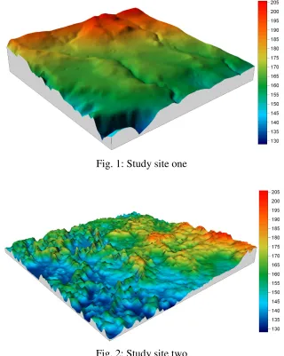
The study area is in the region of Corangamite Catchment Management Authority (CCMA) in south western Victoria, Australia. The landscape in the region can be depicted to north and south highlands and a large Victoria Volcanic Plain (VVP) in the middle. The VVP is dominated by Cainozoic volcanic deposits. It is characterized by vast open areas of grasslands, small patches of open woodland, stony rises denoting old lava flows, numerous volcanic cones and old eruption, and is dotted with shallow lakes both salt and freshwater. Terrain types vary between the comparatively treeless basins of internal drainage on Victoria Volcanic Plains (VVP) to dissected terrains north and south. The plains have high priority for a range of research projects pertaining to environment management issues addressed in the catchment management strategy plan. LiDAR data from the first stage of CCMA LiDAR project covered an area of 6900 km². In this study, two LiDAR tiles (covered an area of 5 km by 5 km each) were selected as the test sites, shown in Figures 1 and 2. Site one is relative flat, with several shallow gullies. Site two is dominated by volcanic derived stony rises, with rough terrain.
LiDAR Data
LiDAR data were collected over the period of 19 July 2003 to 10 August 2003. The primary purpose of this LiDAR data collection was to facilitate more accurate terrain pattern representation for the implementation of a series of environment related projects. The LiDAR data have been classified into ground and non-ground points by using data filter algorithms across the project area. Manual checking and editing of the data led to further improvement in the quality of the classification. The resulting data products used for DEM generation are irregularly distributed LiDAR ground points, with an average spacing of 2.2 m (AAMHatch 2003). The accuracy of LiDAR data was estimated as 0.5 m vertically and 1.5 m horizontally (AAMHatch 2003). The LiDAR data were delivered as tiles in ASCII files containing x, y, z coordinates and intensity values.
Methods
775
datasets for each test site. The elevation value of each check point from test dataset was compared to the correspondent elevation value from DEMs produced at each of data density levels. Root mean square error (RMSE) and mean absolute error were calculated to assess the performance of different interpolation algorithms at different LiDAR data density levels.
[image:5.595.138.458.154.555.2]Fig. 1: Study site one
Fig. 2: Study site two
776
RESULTS AND DISCUSSION
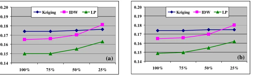
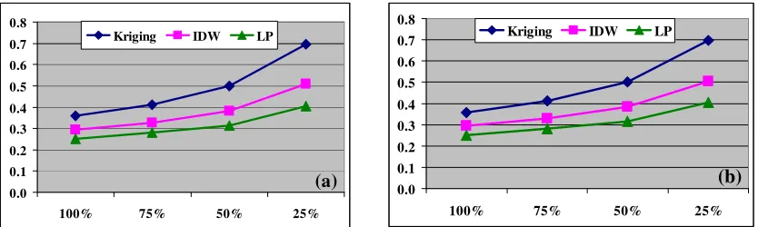
RMSEs obtained from validation and cross-validation with different interpolators at various LiDAR density levels for site one and site two are presented in Table 1, and depicted in Figures 3 and 4 as well. At all LiDAR density levels, both validation and cross-validation showed that local polynomial method has the lowest RMSE values at site one and site two. Compared to IDW and Kriging, the local polynomial performed extremely well on flat terrain (site one). Kriging usually gave the biggest RMSEs with exception at 25% data density for site one.
RMSEs from all three interpolation algorithms increased with the decrease of LiDAR data density at both test sites. However, there is only slight increase of RMSEs with Kriging from both validation and cross-validation, indicating that Kriging is insensitive to data density on a flat terrain like the test site one. On a complex terrain (site two), all three interpolation algorithms are sensitive to data density, showing significant increases when LiDAR data density decreased from 100% to 25%. Even on flat terrain (site one), both IDW and local polynomial algorithms are sensitive to data density, being significant when density decreasing from 75% to 25% of the original data.
On flat terrain, RMSEs from all three interpolation algorithms are smaller than those corresponding to complex terrain. For example, with cross-validation at 100% LiDAR data density, the local polynomial yielded a RMSE of 0.149 m at site one, and 0.250 m at site two. It gave an indication that terrain type has a significant impact on interpolation results. On flat terrain, interpolators performed well, while on complex terrain, interpolation process may introduce more errors, even in the case of high-density sampling data.
Tab.1: RMSEs obtained from validation and cross-validation with different interpolators at various LiDAR density levels for site one and site two
Site one Site two
Density Interpolator Validation
Cross-validation Validation
Cross-validation
100%
Kriging 0.174 0.174 0.358 0.411
IDW 0.165 0.165 0.294 0.296
LP 0.150 0.149 0.250 0.250
75%
Kriging 0.174 0.174 0.411 0.282
IDW 0.166 0.166 0.327 0.328
LP 0.150 0.150 0.282 0.282
50%
Kriging 0.175 0.175 0.500 0.500
IDW 0.170 0.170 0.382 0.383
LP 0.155 0.155 0.315 0.317
25%
Kriging 0.176 0.175 0.694 0.696
IDW 0.181 0.180 0.508 0.505
777
Kriging was originally developed to estimate the spatial concentrations of minerals for the mining industry. Kriging takes into account both the distance and the degree of variation between sampling data. From a statistical perspective, Kriging is a sound method (Lu and Wong 2008). In practice, however, it may not satisfy users. This study demonstrated that Kriging did not work well for LiDAR data on both flat and complex terrains. Furthermore, it is not a quick interpolator, consuming more computer resources, especially for large volume of LiDAR data. The local polynomial interpolation fits the specified order (zero, first, second, third, and so on) polynomial using points within the defined neighbourhood. It is a moderately quick interpolator (ESRI 2008). In our study, it provided better results than other two algorithms on flat terrain.
The IDW interpolation assumes the closer a sample point is to the prediction location, the more influence it has on the predicted value. It estimates a point value using a linear-weighted combination set of sample points. The weights assigned depend only on the distances between the point locations and the particular location to be estimated, but the relative locations between sampling data are not considered (Myers 1994). Therefore, the use of IDW is straightforward and non-computationally intensive (Lu and Wong 2008). The IDW works well for dense and evenly distributed sample data (Childs 2004). This study showed that even on complex terrain, IDW can produce good results, without significant difference with those from the local polynomial. Considering its simplicity, quick computation and availability in almost all the GIS software, IDW is the most suitable interpolation method for LiDAR data.
0.14 0.15 0.16 0.17 0.18 0.19 0.20
100% 75% 50% 25%
Kriging IDW LP
(a)
0.14 0.15 0.16 0.17 0.18 0.19 0.20
100% 75% 50% 25%
Kriging IDW LP
[image:7.595.93.509.425.549.2](b)
778
0.0 0.1 0.2 0.3 0.4 0.5 0.6 0.7 0.8
100% 75% 50% 25%
Kriging IDW LP
(a) 0.00.1 0.2 0.3 0.4 0.5 0.6 0.7 0.8
100% 75% 50% 25%
Kriging IDW LP
[image:8.595.92.509.71.196.2](b)
Fig. 4: RMSEs from different interpolators at various LiDAR density levels for site two, (a) using validation, (b) using cross-validation
CONCLUSION
Relative vertical accuracy of DEMs may be more important than absolute vertical accuracy in some applications. Selection of an appropriate interpolator could be critical for DEM generation as it is an important factor affecting the relative vertical accuracy of the DEM. This study used validation and cross-validation to evaluate the performance of IDW, Kriging and local polynomial algorithms for LiDAR data on two different terrains. Results showed that Kriging did not work well. The local polynomial performed much better than IDW on flat terrain, but there was no significant difference with IDW on complex terrain. Accuracies from interpolators became worse with the decrease of LiDAR data density, with Kriging being insensitive to data density on flat terrain. As a trade-off between accuracy and computing time for large volume of LiDAR data, IDW is the recommended interpolation method for DEM generation from LiDAR data.
REFERENCES
AAMHatch. 2003. Corangamite CMA airborne laser survey data documentation. AAMHatch Pty Ltd, Melbourne, Australia, 10 p.
ASPRS. 2004. ASPRS Guidelines, Vertical Accuracy Reporting for LiDAR Data. Arerican Society for Photogrammetry and Remote Sensing (ASPRS) Bethesda, Maryland, USA, 20 p.
Burrough, P. A. and McDonnell, R. A. 1998. Principles of Geographical Information Systems, Oxford: Oxford University Press.
Childs, C. 2004. Interpolation surfaces in ArcGIS spatial analyst. ArcUser, July-September:32-35.
El-Sheimy, N., Valeo, C. and Habib, A. 2005. Digital terrain modeling: acquisition, manipulation, and application, Boston and London: Artech House.
ESRI. 2008. Using ArcGIS Geostatistical Analyst. Environmental Systems Research Institute, Redlands, CA, USA, 300 p.
Fisher, P. F. and Tate, N. J. 2006. Causes and consequences of error in digital elevation models. Progress in Physical Geography, 30(4):467-489.
779
ICSM. 2008. ICSM Guidelines for Digital Elevation Data. Inter-Governmental Committee on Surveying and Mapping (ICSM), Canberra, Australia, 49 p.
Jensen, J. R. 2007. Remote Sensing of the Environment: an Earth Resource Perspective, Upper Saddle River, NJ: Pearson Prentice Hall.
Li, Z., Zhu, Q. and Gold, C. 2005. Digital Terrain Modeling: Principles and Methodology, Boca Raton, London, New York, and Washington, D.C.: CRC Press. Liu, X. 2008. Airborne LiDAR for DEM generation: some critical issues. Progress in
Physical Geography, 31(1):31-49.
Lloyd, C. D. and Atkinson, P. M. 2002. Deriving DSMs from LiDAR data with kriging.
International Journal of Remote Sensing, 23(12):2519-2524.
Lloyd, C. D. and Atkinson, P. M. 2006. Deriving ground surface digital elevation models from LiDAR data with geostatistics. International Journal of Geographical Information Science, 20(5):535-563.
Lohr, U. 1998. Digital elevation models by laser scanning. Photogrammetric Record, 16:105-109.
Lu, G. Y. and Wong, D. W. 2008. An adaptive inverse-distance weighting spatial interpolation technique. Computer and Geosciences, 34:1044-1055.
Maune, D. F. 2007. DEM User Requirements. In Maune, D. F. (Eds.), Digital Elevation Model Technologies and Applications: The DEM Users Manual, 2nd Edition, Bethesda, Maryland: American Society for Photogrammetry and Remote Sensing. 449-473.
Myers, D. E. 1994. Spatial interpolation: an overview. Geoderma, 62:17-28. NDEP. 2004. Guidelines for digital elevation data, Version 1.0,
http://www.ndep.gov/NDEP_Elevation_Guidelines_Ver1_10May2004.pdf, National Digital Elevation Program (NDEP). (accessed 18 January 2009).
Ramirez, J. R. 2006. A new approach to relief representation. Surveying and Land Information Science, 66(1):19-25.
Turton, D. A. 2006. Factors Influencing ALS Accuracy. AAMHatch Pty Ltd, Brisbane, Australia, 5 p.
Weydahl, D. J., Sagstuen, J., Dick, Ø. B. and Rønning, H. 2007. SRTM DEM accuracy assessment over vegetated areas in Norway. International Journal of Remote Sensing, 28(16):3513-3527.
Zimmerman, D., Pavlik, C., Ruggles, A. and Armstrong, M. P. 1999. An experimental comparison of ordinary and universal Kriging and inverse distance weighting.
Mathematical Geology, 31(4):375-389.
BRIEF BIOGRAPHY OF PRESENTER