MW_Thesis.pdf

(1)

Abstract

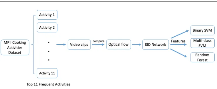
This project focuses on using Machine Learning methods to recognize actions from cooking video sequences. The cooking videos and annotations are from MPII Cooking Activities Dataset, and a subset was constructed by selecting a group of the most frequently appearing actions, and generating matching video clips. Optical flows of those 11 actions’ videos were computed and were passed into a pre-trained Deep Learning Two-Stream Inflated 3D ConvNet to generate features of dimension 1024. Support Vector Machine classifiers and Random Forest classifiers were then applied to recognize and classify these actions using the extracted features. Binary SVM had the worst performance among the three classifiers we tested, whether

(2)

1. Introduction

The rapid growth of social media and the development of technology like Internet of Things (IoT) has resulted in the availability of food related digital data. At the same time, more studies in food computing have been carried out [1]. Food data can be in various formats, i.e. text (food recipe), pictures, and videos. Research on digital food data ranges from recognition and segmentation of images/videos to recipe retrieval and estimation [1].

Our eventual goal is the creation of complete recipes from cooking videos. For the purpose of this thesis, we focus only on recognizing cooking actions in cooking videos, as an appropriate starting point. There are many publically available datasets of cooking videos, including MPII Cooking Activities Dataset [2], Breakfast Dataset [3], and YouCook2 Dataset [4]. After considering the complexity of the data sets, the level of annotation available, and availability of a sufficient number of examples of each cooking action, we constructed a customized set of video clips of cooking activities from the MPII Cooking Activities Dataset. From this subset we extracted short video clips, with each one representing a single cooking activity that was used in the action recognition task.

Action recognition from video data is an important topic in computer vision. There have been various structures developed to complete the task, and [5] examined and compared some of them. It is also presented in [5] that an architecture trained on a large dataset beforehand could improve the performance when applying to other datasets. We used the Two-Stream Inflated 3D ConvNets (I3D) developed by [5] with the Kinetics Human Action Video Dataset [6] to generate features from the cooking video clips.

(3)

action. The complete workflow of this project is presented in Figure 1.

(4)

2. Data for cooking action recognition

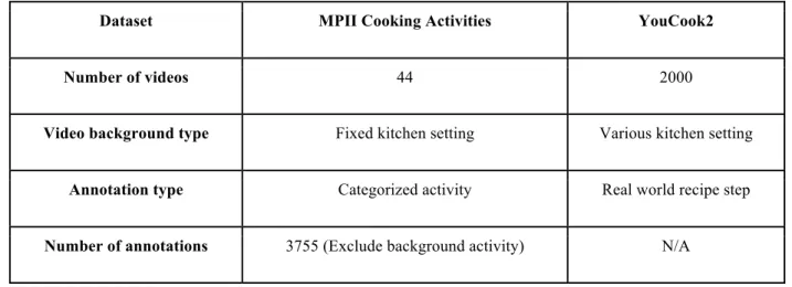
MPII Cooking Activities Dataset [2] and YouCook2 Dataset [4] were the two potential datasets to be used for the task of cooking video recognition. These two datasets differ in data size, video type, annotation type, etc. as shown in Table 1. We decided MPII was better suited to be used for this project because of the categorized activities annotations, which work better for classification task, and the consistency in video background and video quality.

Dataset MPII Cooking Activities YouCook2

Number of videos 44 2000

Video background type Fixed kitchen setting Various kitchen setting

Annotation type Categorized activity Real world recipe step

Number of annotations 3755 (Exclude background activity) N/A Table 1. Attributes of MPII Cooking Activities and YouCook2 data set

MPII consists of a total of 44 videos recorded under the same kitchen setting and none of the videos have audio. The videos are shot with a camera system from 4D View Solutions at 30 frames/sec.

The length of these videos ranges from 2.72 minutes to 40.72 minutes, with a total of 64 categories of activities and a total of 3,755 activity annotations, excluding the category 1

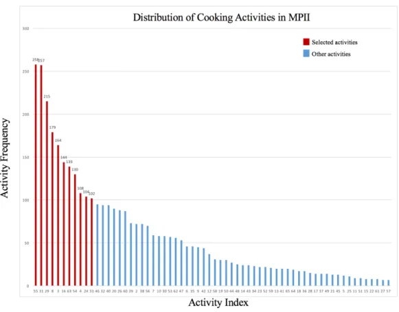
background activity. The distribution of the categorized activities is shown in Figure 2, with the highest frequency action with 258 appearances and the lowest frequency action with 7

(5)

Figure 2. Distribution of cooking activities (excluding background activity) in MPII

Index Activity Frequency Index Activity Frequency

55 Take out from drawer 258 63 Wash objects 139

31 Put on bread/dough 257 54 Take out from cupboard 130

29 Put in bowl 215 4 Cut dice 108

8 Cut slices 179 24 Peel 104

3 Cut apart 164 33 Put on plate 102

16 Move from X to Y 144

Table 2. Selected activities and their frequencies

(6)

(7)

3. Methods

3.1 Feature Generation

3.1.1 Computation of Optical Flow

As shown in Figure 1, the first step in the processing was to compute the optical flow of each video clip. Optical flow is the G, and the computation of classical optical flows without motion discontinuities is based on two assumptions: (a) the intensity of pixels will not change between two consecutive frames; and (b) neighboring pixels will have similar motion between frames. Different methods can be implemented to compute optical flows. For example, the Lucas-Kanade method, a sparse flow computation method, computes optical flows for chosen points/features in an image [7], while a dense optical flow computation method such as the one developed by Gunnar Farneback calculates the flow for every point in an image [8].

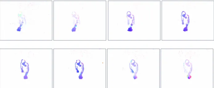
For this specific project, we implemented the duality based approach [9] that calculates dense optical flows to fit with the neural network that we were going to use. This is also an approach that could capture motion discontinuities. Figure 3 visualizes the optical flow of a sample video clip from activity category “Move from X to Y”. Any video clip that has less than 20 frames was omitted in the later work. The outputted optical flow was a tensor shaped as (1, N, 224, 224, 2) where N is the number of frames, 224s are the video width and height (after

(8)

Figure 3. Visualization of an optical flow of a “Move from X to Y” clip

3.1.2 Computation of Feature Vectors using 3D ConvNets

(9)

Figure 4. Structure of I3D Figure 5. Maximum margin of SVM

3.2 Classifier Training and Testing 3.2.1 Train and Test Sets

The complete set of data consists of 1,790 feature arrays, one each from the 1,790 video clips. 90% of the video clips were used as the training data (1,607 in total) with the rest in the test set (183 in total). The initial train/test split was based on all actions, but this random split resulted in some activities being overrepresented than others in the test set. Thus, we ended up with the 90%/10% split being applied to each action individually.

3.2.2 Binary SVM Classifier

The first classifier we tested was the traditional binary Support Vector Machine (SVM) classifier [10]. SVM separates labeled classes with a hyperplane that has the largest possible distance (margin) to the nearest data points of the two classes as shown in Figure 5. We used SVM because it is efficient and although it works best in linear cases, non-linear separation is possible by using various kernels.

(10)

actions labeled as 0. Dividing the whole set into just two classes resulted in an imbalance between the number of positive classes and negative classes, and that imbalance was considered during the training by setting parameter class_weight to be “balanced” mode so that class weights are adjusted inversely proportional to class frequencies.

When the classifiers were tested, all 11 classifiers were used to classify all 11 actions’ test set. For example, all 11 classifiers were used to label the 17 test cases of activity #3, which were not used in training. The expectation was that the classifier trained on activity #3 previously would recognize these actions and return True (1), while other classifiers should return False (0).

3.2.3 Multi-class SVM Classifier

After testing with the binary SVM classifier, we implemented the multi-class SVM classifier to see if it could improve the preformance. Training data and test data were aggregated and labeled according to the activity number, resulted in a total of eleven classes. The multi-class SVM classifier came from the scikit learn library, and both SVC() and LinearSVC() were used. SVC() takes an one-against-one approach [11], which in fact constructs a total of N*(N-1)/2 binary classifiers for every pair of classes with N being the number of total classes. On the other hand, LinearSVC() is trained directly on a one-against-other basis, and only one model is constructed during the process.

3.2.4 Random Forest Classifier

(11)

subsets of features.

The package used in the project also came from the scikit learn library. A Random Forest Classifier with default settings was used first to set the baseline performance. We used

(12)

4. Results

4.1 Binary SVM Classifier

The first trial of Binary SVM did not yield good results. The accuracy for a classifier trained on Activity #N to predict #N as the output is not high enough (see detailed result in Table 2 in the Appendix), with a lower bound of only 0.27 (Activity #4 “Cut dice”). More than that, there are also misclassification cases from other classifiers, i.e. a classifier trained on Activity #M predicted #N to be True (1) (M N).

It turned out that the problem might be the unbalanced situation when training each of the classifiers. The second trial corrected such an imbalance, and the rate for specific classifier to accurately predict that activity has been increased (see detailed result in Table 3 in the

Appendix). The true positive rate for all 11 classifiers was 0.85, with a lower bound of 0.64 for the classifier trained on activity #33 “put on plate.” However, the number of misclassification cases between unmatched classifiers and activities also increased, especially for classifiers trained on activity #3 “cut apart,” activity #29 “put in bowl,” and activity #33 “put on plate.”

4.2 Multi-class SVM Classifier

(13)

4.3 Random Forest

A random forest classifier with default settings was first applied, with the prediction result presented in Table 6 in the Appendix. The average precision rate was 0.65, which was lower than the performance of multi-class SVM classifier and thus not optimal.

To improve performance, we first tried to search for individual optimized hyper-parameters. Hyper-parameters that we considered to adjust include: number of estimators (“trees”), maximum depth of the tree developed, and minimum number of samples required to split an internal node. These hyper-parameters decide the complexity of the classifier, and the classifier could be over fitted without these restrictions.

A sample output of the search for the best number of estimators to be used is shown in Figure 6. However, it turned out that optimized individual parameters have the potential problem of overfitting. They might not result in an optimized performance when grouped together, and manually going over all possible hyper-parameter combinations was impossible. Thus, we

implemented RandomizedSearch to finish the task, and the resulting combination was as follows: number of estimators = 512, minimum samples split = 5, maximum depth = 80.

(14)

Figure 6. Train and test results when tuning hyper-parameter n_estimator.

(15)

5. Conclusion and Future Work

Comparing the results from the three classifiers we implemented: binary SVM, multi-class SVM, and random forest, we observed a poor performance in binary SVM, with low true positive rate when not considering the imbalance between two classes, and high false positive rate when considering the imbalance. Multi-class SVM classifier and random forest classifier performed approximately equally well, both having an average precision at around 0.8.

From the test it seemed that the number of video clips is sufficient for the classification task, with each activity having at least 100 video clips for training and testing. More training data may allow for better performance, but due to the limit of the original data set it was not

applicable. The features generated by the I3D network also seemed appropriate to be used in classification, but we could pass videos into other video structures and compare the results for further research. If there were more samples to be used, we could also retrain the I3D network first, or we could consider build and train a structure from scratch.

(16)

Bibliography

[1] W. Min, S. Jiang, L. Liu, Y. Rui, and R. Jain. A Survey on Food Computing. arXiv preprint arXiv:1808.07202, 2018.

[2] M. Rohrbach, S. Amin, M. Andriluka, and B. Schiele. A Database for Fine Grained Activity Detection of Cooking Activities. In CVPR, 2012.

[3] H. Kuehne, A. Arslan, and T. Serre. The Language of Actions: Recovering the Syntax and Semantics of Goal-Directed Human Activities. In CVPR, 2014.

[4] L. Zhou, C. Xu, and J. J. Corso. Towards Automatic Learning of Procedures from Web Instructional Videos. arXiv preprint arXiv: 1703.09788. 2017.

[5] J. Carreira, and A. Zisserman. Quo Vadis, Action Recognition? A New Model and the Kinetics Dataset. In CVPR, 2017.

[6] W. Kay, J. Carreira, K. Simonyan, B. Zhang, C. Hillier, S. Vijayanarasimhan, F. Viola, T. Green, T. Back, P. Natsev, M. Suleyman, and A. Zisserman. The kinetics human action video dataset. arXiv preprint arXiv:1705.06950, 2017.

[7] B.D. Lucas, and T. Kanade. An Iterative Image Registration Technique

with an Application to Stereo Vision. In Proceedings of Imaging Understanding Workshop, pages 121 – 130. 1981.

[8] G. Farneback. Two-Frame Motion Estimation Based on Polynomial Expansion. In Scandinavian Conference on Image Analysis, 2003.

[9] C. Zach, T. Pock, and H. Bischof. A Duality Based Approach for Realtime TV-L1 Optical Flow. In Pattern Recognition, pages 214–223. Springer, 2007.

[10] C. Cortes, and V. Vapnik. Support-vector networks. In Machine Learning, vol. 20, no. 3,

(17)

[11] S. Knerr, L. Personnaz, and G.Dreyfus. Single-layer learning revisited: A stepwise procedure for building and training neural network. In Neurocomputing: Algorithms, Architectures and Applications, pages 41–50. Springer, 1990.

(18)

Appendix Actual number of video clips of each activity

Index Activity Frequency Index Activity Frequency

55 Take out from drawer 258 63 Wash objects 139

31 Put on bread/dough 257 54 Take out from cupboard 130

29 Put in bowl 205 4 Cut dice 108

8 Cut slices 179 24 Peel 104

3 Cut apart 164 33 Put on plate 102

16 Move from X to Y 144

(19)

Binary SVM Classifier: not consider unbalanced case Classifier \Action 3 Cut apart 4 Cut dice 8 Cut slices 16 Move from X to Y

24 Peel 29 Put in bowl 31 Put on bread/dou gh 33 Put on plate 54 Take out from cupboard 55 Take out from Drawer 63 Wash Objects

3 6 1 1 1

4 2 3 2

8 1 11

16 9 1 1 1

24 7

29 1 1 16 1 1

31 18 3

33 1 1 4

54 13

55 1 26

63 2 13

Actual 1 17 11 18 15 11 21 26 11 13 26 14

(20)

Binary SVM Classifier: consider unbalanced case Classifier \Action 3 Cut apart 4 Cut dice 8 Cut slices 16 Move from X to Y

24 Peel 29 Put in bowl 31 Put on bread/dou gh 33 Put on plate 54 Take out from cupboard 55 Take out from Drawer 63 Wash Objects

3 12 5 3 1 1 2 1 1

4 4 10 5

8 2 7 17 1 1

16 11 4 1 1 1

24 10 1

29 1 1 1 1 17 2

31 1 1 20 4 1

33 2 1 1 1 3 7 1

54 13

55 1 26

63 2 13

Actual 1 17 11 18 15 11 21 26 11 13 26 14

(21)

Multi-class SVM Classifier: one-against-one

Precision Recall Support

3 Cut apart 0.45 0.29 17

4 Cut dice 0.00 0.00 11

8 Cut slices 0.40 1.00 18

16 Move from X to Y 0.63 0.80 15

24 Peel 1.00 0.18 11

29 Put in bowl 0.89 0.38 21

31 Put on bread/dough 0.46 0.81 26

33 Put on plate 0.00 0.00 11

54 Take out from cupboard 0.93 1.00 13

55 Take out from drawer 0.96 0.92 26

63 Wash objects 0.92 0.79 14

Average / Total 0.63 0.62 183

Table 4

Multi-class SVM Classifier: one-versus-the-rest

3 Cut apart 0.69 0.53 17

4 Cut dice 0.46 0.55 11

8 Cut slices 0.68 0.83 18

16 Move from X to Y 0.87 0.87 15

(22)

29 Put in bowl 0.81 0.81 21

33 Put on plate 0.67 0.55 11

63 Wash objects 0.93 0.93 14

Table 5

Random Forest Classifier: default setting

3 Cut apart 0.38 0.47 17

4 Cut dice 0.40 0.18 11

8 Cut slices 0.62 0.83 18

16 Move from X to Y 0.59 0.87 15

24 Peel 0.88 0.64 11

29 Put in bowl 0.64 0.67 21

33 Put on plate 0.50 0.09 11

63 Wash objects 0.70 0.50 14

(23)

Random Forest Classifier: tuned hyper-parameters

3 Cut apart 0.62 0.59 17

4 Cut dice 1.00 0.18 11

8 Cut slices 0.69 1.00 18

16 Move from X to Y 0.59 0.87 15

24 Peel 1.00 0.91 11

29 Put in bowl 0.76 0.76 21

33 Put on plate 1.00 0.18 11

63 Wash objects 1.00 0.64 14