Sharif University of Technology
Scientia IranicaTransactions B: Mechanical Engineering www.scientiairanica.com
Estimation of local heat transfer coecient in
impingement jet by solving inverse heat conduction
problem with mollied temperature data
S.D. Farahani
a;, F. Kowsary
aand J. Jamali
ba. Center of Excellence in Design and Optimization of Energy Systems, School of Mechanical Engineering, College of Engineering, University of Tehran, Tehran, Iran.
b. Department of Mechanical Engineering, Shoushtar Branch, Islamic Azad University, Shoushtar, Iran. Received 21 July 2012; received in revised form 8 March 2014; accepted 8 April 2014
KEYWORDS Heat transfer coecient; Impingement jet; Sequential function specication method; Conjugate gradient method;
Mollication method.
Abstract. The aim of this paper is to determinate local convective heat transfer coecient slot jet impingement using inverse heat conduction methods. The sequential specication function method and the conjugate gradient method are used to solve the Inverse Heat Conduction Problem (IHCP) and estimate the space-variable convective heat transfer coecient. This paper proposes a procedure to smooth the temperature data by the mollication method prior to utilizing the inverse method. The measured transient temperature data may be obtained from locations inside the body or on its inactive boundaries. The uncertainties in the estimated heat transfer coecient are calculated using bias and variance errors. The obtained results show that mollifying measured data causes an increase in the accuracy and stability of the estimation.
© 2014 Sharif University of Technology. All rights reserved.
1. Introduction
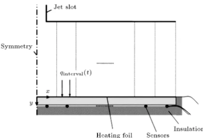
Jet impingement is widely used in industry because of the highly favorable heat transfer rate it provides. Engineering applications include annealing of metal sheets, drying of textile products, deicing of aircraft wings, and cooling of gas turbine blades and elec-tronic components. A case of special interest is the impingement of a turbulent slot jet on a at plate. Figure 1 shows a schematic of dierent zones in this type of jet impingement. Earlier experimental studies have shown that the length of the jet potential core is typically between ve to seven slot widths, and that the maximum heat transfer occurs when the transitional jet hits the plate [1,2]. Mass transfer methods have
*. Corresponding author. Tel.: +98 21 61114024; Fax: +98 21 88013029
E-mail address: [email protected] (S.D. Farahani)
been widely used for many years. The heat-mass transfer analogy, in conjunction with the naphthalene sublimation technique, was used to investigate local and average heat transfer coecients in a two-row plate n and tube heat exchanger with circular tubes [3]. The local mass transfer coecients on this geometry have also been measured by Kruckels and Kottke [4]. They used a chemical method based on absorption, chemical reaction and coupled color reaction [5]. The solid surface is coated with a wet lter paper, and the ammonia to be transferred is added as a short gas pulse. The locally transferred mass is visible as color density distribution and the color intensity corresponds to the local mass ow. Thermo chromic liquid crystals have been applied extensively to heat transfer measure-ments [6-7]. Using temperature maps obtained from liquid crystals applied to a constant heat ux surface, Newton's law of cooling (the boundary condition of the third kind) is used to establish distributions of the convective heat transfer coecient. A constant
Figure 1. Schematic of a turbulent slot jet impinging on a at surface.
heat ux at the body surface is typically generated by passing an electrical current through a n lm with uniform electrical resistivity. Thermo graphic phosphors have also been used for local heat transfer measurements [8,9]. Application of temperature sensi-tive paints to heat transfer measurements is described by Liuo and Sullivan [10]. Optical measurement tech-niques have found widespread application in heat trans-fer investigations [11,12]. Dierential intertrans-ferometry can be used to determine local temperature gradients in the uid and a local heat transfer coecient at the solid surface.
However, these methods either require expensive or delicate equipment or have limitations to high temperatures or high levels of turbulence in the ow. An alternative method that is also particularly suited for the investigation of impingement jet heat transfer is the Inverse Heat Conduction (IHC) technique. It is advantageous because it can be carried out with simple, low-cost instrumentation and subsequent numerical procedures. In this technique, temperatures measured at some proper interior locations are used to estimate a thermal boundary condition. The word \estimation" is used here as temperature measurements always contain noise. The Inverse Heat Conduction Problem (IHCP) is mathematically \ill-posed" in the sense of Hadamard [13], and this causes the IHCP to be partic-ularly sensitive to measurement errors. The IHCP can be classied according to factors, such as (1) linearity, (2) the time domain used (sequential vs. whole domain), and (3) dimensionality. Many investigators have developed various inverse schemes over the past 40 years. Tikhonov's regularization technique [14] and Beck's function estimation method [15] are among the most well-known approaches in inverse heat transfer. Another method that has been widely used is the con-jugate gradient method (see, e.g. [16]), which belongs to the class of iterative regularization techniques. Masson et al. [17] applied iterative regularization and Function Specication Methods (FSMs) with a spatial regular-ization to estimate the two-dimensional heat trans-fer coecient. Taler [18] compared two techniques,
Singular Value Decomposition (SVD) and Levenberg-Marquardt used in determining the space variable heat transfer coecient on a tube circumference. Good agreement was found between the results in a simulated experiment. Guzik and Styrylska. proposed the gen-eralized optimal dynamic ltration method, developed on the Unied Least-Squares Method (ULSM) with the use of the multistage-multi group (M-M) technique, for the mathematical modeling of transient temperature elds, using data subject to uncertainties [19]. Kowsary and Farahani [20] applied denoised measurement data using the mollication method before the standard IHCP algorithm for estimated heat ux for classical inverse problems. The purpose of this study is to use the solution of a transient, sequential IHC scheme (sequential function specication method) [13] and iter-ative scheme (conjugate gradient method) [16] with and without denoised data, using the mollication method, to estimate distribution of the steady-state convective heat transfer coecient in a slot jet impingement. The method is required to be considered two-dimensional because of the lateral conduction that occurs between the warmer and cooler areas of the surface of the target plate, which, in many investigations using a thermocouple, was disregarded. Due to the existence of lateral conduction within stainless steel, the local heat transfer coecient was corrected to include this eect. The correction was performed regarding a two-dimensional model.
The mollication method is used for smoothing the simulated measurement in simulation for estima-tion of the heat transfer coecient.
2. Problem description
To use the inverse scheme, rstly, the direct problem should be formulated. The governing dierential equa-tion is the following two dimensional transient heat conduction equations solved in the mid-plane (z = 0) of the target plate (Figure 2). Assuming constant thermal
Figure 2. Schematic of the experiment set-up for inverse method.
properties: @2T
@x2 +
@2T
@y2 =
1
@T @t; @T
@xjx=0= @T
@xjx=L1=
@T
@yjy=L2= 0;
k@T@yjy=0= q(x; t) and T jt=0= T0; (1)
where T0 is the initial temperature of the plate (=
room/surrounding temperature), and L1 and L2 are
half-plate length and plate thickness, respectively. In the inverse problem, the boundary condition on the top (y = 0) surface, q(x; t), is unknown; instead, some temperature measurements at discrete times and locations are given:
Yj;i= Tmeas(xj; ti); (2)
where i and j are measurement time and number of sensor indices, respectively. In the estimation of the heat transfer coecient, two approaches can be used: (a) the direct estimation and (b) the estimation of q(x; t), subsequent calculation of Tsurf(x; t), and
then using Newton's law of cooling. While direct estimation might seem more appealing, the second approach causes the IHCP to remain linear, thus, eliminating the need for iteration, which accelerates the solution considerably. Note that in the present set-up, a heating foil generates a constant known heat ux of Qson the top surface. A part of Qs, namely q(x; t), is
conducted into the solid and estimated by the IHCP. The heat transfer coecient is then calculated using the remaining part, which is carried away by the jet, using Newton's law of cooling:
h(x) =TQs q(x; t)
surf(x; t) Tjet; (3)
where Tsurf(x; t) and Tjet are the top surface and
the jet exit temperatures, respectively. For solving the inverse heat conduction problem, two methods were employed, namely, the Sequential Function Spec-ication Method [13] and the Conjugate Gradients Method [16].
The dierential equation for X is obtained from the direct dierentiation of the governing heat con-duction equation with respect to q. This way of calculating X is particularly suited for this study, since, in the presence of linearity, sensitivity coecients will be independent of unknown parameters, that is, once calculated, they remain constant in the course of the inverse procedure. Based on this description, the sensitivity equations are as follows:
@2X
@x2 +
@2X
@y2 =
1
@X @t ; @X
@xjx=0= @X
@xjx=L1=
@X
@yjy=L2 = 0;
k@X@yjy=0=
8 > < > :
1 xn< x < xn+1
; Xjt=0= 0
0 otherwise (4)
3. Method description
3.1. The Conjugate Gradients Method (CGM) In order to estimate the heat ux using the conjugate gradients method, the error function S is also dened as:
S(q) =XNs
i=1 Nm
X
m=1
(Ti(tm) Yi(tm))2; (5)
where Y is measured temperatures at the sensor loca-tion and T is the estimated value at the sensor localoca-tion. In Eq. (5), NS refers to the number of temperature sensors. The directional derivative of S can be used to dene the gradient function of rS, with respect to Q, as follows:
~rS = 2[X]T([Y ] [T ]) ; (6)
where all the mentioned parameters are evaluated at the sensor location. Using the above equation, the conjugate direction (d) can be calculated as:
dk = rS(Qk) + kdk 1: (7)
The conjugate coecient, , is calculated as:
k=Z tf
t=0frS(Q
k)g2dt=Z tf
t=0frS(Q
k 1)g2dt;
(8) where 0 = 0. If Q0 = Qk + dk is substituted in
Eq. (1), then, values T will be calculated at the sensor location, as follows:
T = T (Q0) T (Qk): (9)
Therefore, the search step size () can be obtained as:
k=
0 @XJ
j=1 M
X
m=1
Tj(tm) Yjm(tm)Tj(tm)
1 A = 0
@Xk
j=1 M
X
m=1
T2 j(tm)
1 A :
In this method, an iterative procedure is used to estimate the imposed heat ux. This iterative method can be summarized by the following equation:
Qk+1= Qk kdk; (11)
where \d" is a conjugate direction and is the search step size. The computational procedure for the solution of this inverse problem may be summarized as follows: Suppose Qn is available at iteration n.
Step 1. Solve the direct problem given by Eq. (1) for T .
Step 2. Examine the stopping criterion, considering S(Q) < , where is a small-specied number. Continue if not satised.
The \Discrepancy Principle" method in the con-jugate gradient method has been used in this study. In this method, the iterations are terminated prematurely when the following criterion is satised [16]:
S(Q) < : (12)
In this case, the iterations are stopped when the residu-als between measured and estimated temperatures are of the same order of magnitude as the measurement errors. That is:
jY (t) T (X; t)j < (i.e. standard deviation): (13) Step 3. Solve the sensitivity equation given by Eq. (4) for X.
Step 4. Compute the gradient of the functional rS from Eq. (6).
Step 5. Compute the conjugate coecient, k,
and direction of descent, dk, from Eqs. (7) and (8),
respectively.
Step 6. Set rQ = dk in Eq. (1), and solve for
calculated T .
Step 7. Compute the search step size, k, from
Eq. (10).
Step 8. Compute the new estimation for Qn+1 from
Eq. (11) and return to Step 1.
3.2. The Sequential Function Specication Method (SFSM)
This inverse method is sequential and uses Beck's function specication approach, where heat uxes of r \future" time steps are temporarily assumed constant
and used to add stability to the estimations. It is assumed that heat uxes from time 1; 2; ::; (m 1) are estimated, and now the unknowns in time m are to be evaluated. The standard form of the IHCP is the matrix equation (see [13]):
T = T jq=0+ Xq; (14)
where T jq=0 is the calculated temperatures at sensor
locations from the solution of the direct problem using q1; :::; qm 1 and setting Eq. (7a) to zero for Np heat
ux parameters, Ns temperature sensors, and r future times: T = 2 6 6 6 4 T (m) T (m + 1)
... T (m + r 1)
3 7 7 7
5 and T (i) = 2 6 6 6 6 6 6 4
T1(i)
... T2(i)
... TNs(i)
3 7 7 7 7 7 7 5 ; (15)
where T is an Ns:r 1 matrix:
q = 2 6 6 6 4 q(m) q(m + 1)
... q(m + r 1)
3 7 7 7
5 q(i) = 2 6 6 6 4
q1(i)
q2(i)
... qNp(i)
3 7 7 7
5; (16)
where T is an Np:r 1 matrix, and:
Z = 2 6 6 6 4 a(1) a(2) a(1) ... ... ... a(r) a(r 1) a(1)
3 7 7 7
5; (17)
where Z is an Ns:r Np:r matrix, and:
a = 2 6 6 6 4
a11(i) a12(i) a1Np(i)
a21(i) a22(i) a2Np(i)
... ... ... aNs1(i) aNs2(i) aNsNp(i)
3 7 7 7 5;
ajp= @T (x@qj; ti)
p ; (18)
where a(i) is a matrix of Ns Np.
Note that there are Np unknown heat ux compo-nents at each time, tm. There are Ns measurements at
that time, and Ns must be no less than Np. To produce stable results, we use r matrix equations in a least squares method. The sum of squares of the dierence between calculated and measured temperatures, in matrix form, is:
with the temporary assumption of:
q1(m) = q1(m + 1) = ::: = q1(m + r 1):
::::::qNp(m) = qNp(m + 1) = ::: = qNp(m + r 1):
(20) Here, the function to minimize is:
S = (Y T jq=0 Zq)T(Y T jq=0 Zq) ; (21)
where:
Z = XA; A = 2 6 4
A(1) ... A(r)
3 7
5 : (22)
For a constant q assumption A(i) = INpNp where I is
unity matrix.
The matrix derivative of Eq. (20), with respect to q (in order to minimize S), yields the estimator equation:
^q = ZTZ 1ZT(Y T jq = 0) ; (23)
which gives the ^q(m) vector as dened by Eq. (14). The following estimation procedure is employed: X and, consequently, Z are calculated, and m is set to one. Estimation begins with the calculation of T jq=0
using the direct problem and subsequent application of Eq. (22). Then, m is increased by one, T jq=0 is
recalculated, and the estimator equation is used again. 3.3. The mollication method
Use of the mollication method is discussed more thoroughly, as it is the central subject of this article. The mollication method is a regularization method that uses the averaging property of the Gaussian kernel to smooth noisy data. The automatic character of the mollication algorithm, which makes it highly compet-itive, is due to the incorporation of the Generalized Cross Validation procedure for selection of the radius of mollication as a function of the perturbation level in the data, which is generally not known. The mathematical form of the mollication method was detailed in Ref. [19] and will not be repeated here. Note that we used the mollication method as preltering for denoising measurement data before the inverse algorithm.
The impingement surface is divided into a number of sub-intervals (see Figure 2). The aim is to estimate the time-variable heat ux, qinterval(t), on each interval
and subsequent calculation of the local convective heat transfer coecient. The inverse methods employed are sequential and use Beck's function specication approach and conjugate gradient method. The key factors in an experimental design are measurement
time-step size. Minimizing the time steps, for example, causes measurement errors to become correlated, which introduces instability into the results. High correla-tion between temperature data implies that each new measurement is providing less information than if the correlation was zero. Bias (index of deviation from the actual value), variance (index of intensity of uctua-tions), and sensitivity coecients are good judgment parameters in determining the best experimental set-up. The nal target of the estimations is the heat transfer coecient on each interval. For each interval, bias (D) is dened for the IHCP as:
D = v u u t 1
N
N
X
i=1
^hi;nonoise hi;true
2
; (24)
where ^hi;nonoise noise is the estimated heat ux using
the measurements containing no noise. The Root Mean Square (RMS) error is also calculated by:
RMS = v u u t 1
N
N
X
i=1
^hi;noisydata hi;true
2
; (25)
where ^hi;noisydatadata is the estimated heat ux using
the temperature data polluted with noise. Variance can then be determined by:
V = RMS2 D2: (26)
A series of simulations is performed to ensure the ability of the inverse scheme in estimating the space variable heat transfer coecient and to nd the optimal simulation conguration. Only half of the plate is considered due to symmetry. This half-plate is 10-mm thick, 52.5-10-mm long (7 slot widths), stainless-steel (AISI 304), and insulated on the bottom and side sur-faces (Figure 2). A functional form for the heat transfer coecient is not known a priori, which is the case in many jet impingement heat transfer investigations. The uid temperature, Tjet= T1, is also a known input
to the inverse scheme. After the ow has reached the hydrodynamic steady state, a heat generation source initiates, and, simultaneously, temperature recordings are started using K-type sheathed thermocouples of 1.25-mm diameter. In the present investigation, the heat source is a heating foil applied to the top surface of the plate (when necessary, this source can be of any form; it only requires the appropriate reformulation of the direct problem), and the measurements are carried out at the bottom. This choice of sensor location is most favorable for the experiment's hardware design, since it is simpler in terms of installation; however, it is most challenging for the inverse scheme, since it is farthest from the active surface (resulting in more
\damped" and \lagged" temperature data due to the diusive nature of heat conduction).
Experimental heat transfer coecient data ob-tained from a conned slot jet impingement study [21] is employed, together with the nite element method, to produce the \measured" temperatures. In this paper, the nite element method is used in numerical solutions where ANSYS capabilities are utilized in the mesh generation and numerical solution of the problem, in order to evade the need for coding the direct heat conduction problem. By simulating the problem in the graphic user interface of the software and saving it in the form of a function, the numerical solution of the problem can be performed merely by calling the saved function. Inverse algorithms are written in ANSYS Parametric Design Language (APDL). The element type is Plane-55. A curve tting of seven linear sections was applied to the experimental data of [21] to obtain the continuous heat transfer distribution. The temper-atures at the sensor locations were obtained from the temperature histories at the bottom of the plate. In the inverse heat conduction problem, there are a number of measured quantities in addition to temperature, such as time, sensor location, and specimen thickness. Each is assumed to be accurately known except the temper-ature. The temperature measurements are assumed to contain the major sources of error or uncertainty. Any known systematic eects due to calibration errors, the presence of the sensor, conduction and convection losses, or whatever, are assumed to be removed to the extent that the remaining errors may be considered random. These random errors can then be statis-tically described. In this study, the inverse scheme used is tested using simulated measured temperatures containing Gaussian noise. The following standard assumptions were applied in generating measurement errors: they have a random, additive, and uncorrelated nature with zero mean and constant variance, and they have normal (Gaussian) distribution. Noise with = 0:5 was added to the temperature data.
4. Results and discussion
In this section, the results obtained from simulations are presented. This study emphasizes the use of IHC techniques and ltering for estimating the heat transfer coecient. Among a number of parameter sets that were used for validation of the method, the data for Re=13,600 and H=W = 8 (H and W are the nozzle-to-plate distance and the slot width, respectively) are chosen for presentation of the results in which the ow type is turbulent, as the mentioned methods in the introduction either require expensive or delicate equipment or have limitations to high temperatures or high levels of turbulence in the ow. Note that this method is independent of the ow type, Re and
H=W . This study is performed to ensure the ability of the inverse scheme in estimating the space variable heat transfer coecient. Measurements are carried out until the plate reaches the thermal steady-state condition, which takes approximately 2 minutes. The half-plate is divided into seven equally spaced intervals (Np = 7), and seven sensors are installed at the bottom of the plate beneath each interval. As previously described, interval (t) is estimated for all intervals using the IHCP. Tsurf(x; t) is then calculated, and Eq. (3) is
employed to determine h(x). A test (by the mentioned inverse methods) is performed to demonstrate that the heat transfer coecients are independent of the magnitude of the applied surface heat ux. Note that the \Exact" word in the gures means that the heat transfer coecient for generation of measured temper-ature data is used, and the main aim of the mentioned algorithms is its estimation. The time-average heat transfer coecient on each space interval of the surface is obtained from averaging the estimated heat transfer coecient of that interval in time. Figure 3(a) and (b) illustrate the results for estimation of the heat trans-fer coecient by the sequential function specication method and the conjugated gradient method, where dierent subjected surface heat uxes were used in the numerical experiments. The deviation of results from the so-called \Exact" data is due to the nature of the inverse technique. Figure 3(b) illustrates that the CGM is more accurate than the SFSM. The gures show that the amount of qshas no signicant eect on
the end results.
However, the bias is growing as well, which puts a limit on our choice of r. This trade-o between bias and variance often happens in inverse schemes. The decision concerning factors such as (r) or the time to make measurements is called simulation design. For the present set-up, r = 3 performs the best (see Table 1). A choice of time steps bigger than 1.4 sec is not advisable, as bias is also rapidly growing. In addition, it should be remembered that from the IHCP point of view, a signicant amount of information is lost when we choose too-large time steps. Note that this choice of Tmeas is for the present set-up. It is evident
that if, for example, a more \responsive" material is used as the impingement plate (such as copper), then a much smaller time step would meet the criteria of experiment design. Time step 1.2 sec is chosen to
Table 1. Variation of bias and variance errors with increasing r in SFSM without mollied data.
r Average bias in h(x)
Average variance in h(x)
3 2.696 20.2223
4 3.35 19.8
Figure 3. The estimation average local convective heat coecient by using (a) Sequential Function Specication Method (SFSM) with various Qs, and (b) conjugate Gradient Method (CGM) with various Qs value.
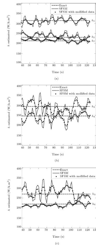
perform. The heat transfer coecient on each interval is constant and calculated in time using Eq. (3). The heat transfer coecient on each interval in time is estimated using the sequential function specication method and the conjugate gradient method with time step 1.2 sec and stopping criterion 1e 6, as shown by Figures 4 and 5, respectively. The uctuations are the consequence of the noise present in the measurements. Earlier times are omitted, since they exhibit the most sensitivity to measurement errors. The eect of noise is also clear from the comparison of Figures 4 and 5. These gures show that by using the mollication method for smoothing measurement data before the IHC algorithm, uctuations in the estimated parameter are reduced. As mentioned earlier, the nal value for the heat transfer coecient on each space interval of the surface is obtained from averaging the estimated
Figure 4. The estimated heat transfer coecients: (a) h1, h5 and h7, (b) h2 and h4, and (c) h3 and h6, in time by using Sequential Function Specication Method (SFSM) with and without mollied data.
Figure 5. The estimated heat transfer coecients: (a) h1, h4, and h7, (b) h2 and h5, and (c) h3and h6, in time by using Conjugate Gradient Method (CGM) with and without mollied data.
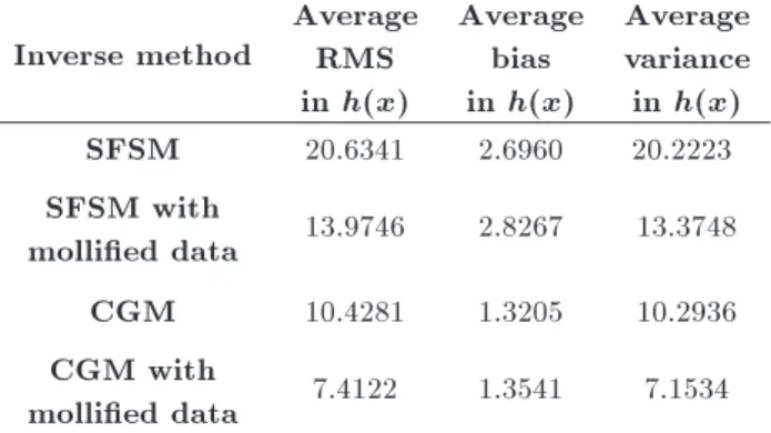
Table 2. Bias and variance errors in SFSM and CGM with and without mollied data.
Inverse method
Average RMS in h(x)
Average bias in h(x)
Average variance in h(x)
SFSM 20.6341 2.6960 20.2223
SFSM with
mollied data 13.9746 2.8267 13.3748
CGM 10.4281 1.3205 10.2936
CGM with
mollied data 7.4122 1.3541 7.1534
heat transfer coecient of that interval in time. It is important that the time step for the mentioned algorithm with mollied data (0.7 sec) be smaller than that without mollied data (1.2 sec). By using the mollied data, we can choose small time steps and achieve more information regarding the estimated parameter.
Figure 3(a) and (b) illustrate the nal results of estimations, when Qs is 8 kW/m2. Table 2 shows
that the RMS value and the variance value are reduced when we use the mollied data. We understand from this table that the conjugate gradient is more accurate than the sequential function specication method. The estimation has the most sensitivity to errors in mea-surement data, but the mollied data has little error. In this method, we must measure only temperature by the thermocouple then use the inverse algorithm for estimation of the local heat transfer coecient. Using an inverse scheme with mollied data for estimation of local heat transfer coecient is a new idea for optimal experiment design.
5. Conclusion
The simulation set up presented in this study works eciently using the inverse scheme to estimate the local convective heat transfer coecient in steady and transient states. The major advantage of the inverse method is that it can be carried out with simple, low cost experimental equipment. A study of sensitivity coecients and a choice of how much bias and variance error is acceptable can be a good start in designing the optimal experiment. Due to the existence of lateral conduction within stainless steel, the local heat transfer coecient was corrected to include this eect. The correction was performed regarding a two-dimensional model. It can be also be concluded that the two dimensional IHCP method (sequential function specication method and conjugate gradient method), especially with mollied measurement data, can suitably be used to design optimum simulation of convective heat transfer coecient estimation before
doing the actual experiment. The temperature mea-surements are assumed to contain the major sources of error or uncertainty. Any known systematic eects due to calibration errors, presence of sensor, conduction and convection losses, or whatever, are assumed to be removed to the extent that the remaining errors may be considered random. It can be seen that by using the mollication method for smoothing measurement data before the IHC algorithm, uctuations in the estimated parameter are reduced and the estimation is more accurate.
Nomenclature
A Vector of unity matrices D Bias error
h Heat transfer coecient (W/m2K)
H Nozzle-to-plate distance H=D h nozzle-to-plate spacing ratio K Thermal conductivity (W/m.K) L1 Half-plate length
L2 plate thickness
M Time index
N Number of discrete measurements Np Number of unknown parameters Ns Number of sensors
q Heat ux vector (W/m2)
Qs Heat ux subjected on top
surface(W/m2)
r Number of future time steps RMS Root Mean Square error S Sum of squares (K2)
d Conjugate direction
T Vector of calculated temperatures V Variance error
W Slot width
X Sensitivity coecient matrix (K=W ) x; y Space coordinates
Y Measured temperature Z XA
Greek symbols
Thermal diusivity (m2/s)
Standard deviation of noise Search step size
Conjugate coecient " Noise value
Subscripts
0 Initial state j Position index jet Jet exit meas Measured
surf Impingement surface
Acknowledgements
This work was partially supported by the Iranian Gas Transmission Company and the Center of Excellence in Design and Optimization of Energy Systems (CE-DOES).
References
1. Choom K.S. and Jim, S.J. \Comparison of thermal characteristics of conned and unconned impinging jets", Int. J. of Heat and Mass Transfer, 53, pp. 3366-3371 (2010).
2. Koseoglu, M.F. and Baskaya, S. \The role of jet inlet geometry in impinging jet heat transfer: Modeling and experiments", Int. J. of Thermal Sciences, 49, pp. 1417-1426 (2011).
3. Kottke, V. and Geschwind, P. \ Heat and mass transfer along curved walls in internal ows", ERCOFTAC Bull, 32, pp. 21-24 (1997).
4. Kruckels, S.W. and Kottke, V. \Investigation of the distribution of heat transfer on ns and nned tube models", Chem. Eng. Technol., 42, pp. 355-362 (1970).
5. Baughn, J.W., Mayhew, J.E., Anderson, M.R. and Butler, R.J. \A periodic transient method using liquid crystals for the measurement of local heat transfer co-ecients", J. Heat Transfer, 119, pp. 242-248 (1998).
6. Wang, Z., Ireland, P.T., Jones, T.V. and Davenport, R. \A color image processing system for transient liquid crystal heat transfer experiments", J. Turbomach, 118, pp. 421-427 (1996).
7. Smits, A.J. and Lim, T.T. Flow Visualization: Tech-niquesand Examples, Imperial College Press, Singa-pore, Eds. (2003).
8. Ervin, J., Bizzak, D.J., Murawski, C., Chyu, M.K. and MacArtur, C. \Surface temperature determination of a cylinder in cross ow with thermographic phosphors", Visualization of Heat Transfer Processes, The Ameri-can Society of Mechanical Engineers, New York, HTD, 252, pp. 1070-1076 (1992).
9. Merski, N.R. \Global aero heating wind-tunnel mea-surements using improved two-color phosphor ther-mography method", J. Spacecr Rockets, 36, pp. 160-170 (1999).
10. Liu, T. and Sullivan, J.P., Pressure and Temperature Sensitive Paints, Springer, Berlin (2005).
11. Lee, D.H., Bae, J.R., Park, J.S., Lee, J. and Ligrani, P. \Conned, milliscale unsteady laminar impinging slot jets andsurface Nusselt numbers", Int. J. of Heat and Mass Transfer, 54, pp. 2408-2418 (2011).
12. Narayanan, V., Seyed-Yagoobi, J. and Page, R.H. \An experimental study of uid mechanics and heat transfer in an impinging slot jet ow", Int. J. of Heat and Mass Transfer, 47, pp. 1827-1845 (2007).
13. Hadamard, J. Lectures on Couchy's Problem in Linear Dierential Equations, Yale University Press, New Haven, CT (1923).
14. Tikhonov, C.R. St. \Inverse problems in heat conduc-tion", J. Eng. Phys., 29, pp. 816-820 (1975).
15. Beck, J.V., Blackwell, B. and Clair, C.R. St. Inverse Heat Conduction: Ill-Posed Problems, Wiley Inter-science, New York (1985).
16. Baonga, J.B., Louahlia-Gualous, J.B. and Imbert, M. \Experimental study of hydrodynamic and heat transfer of free liquid jet impinging a at circular heated disk", Appl. Thermal Eng., 26, pp. 1125-1138 (2005).
17. Masson, P.L., Loulou, T. and Artioukhine, T. \Es-timation of a 2D convection heat transfer coecient during a test: Comparison between two methods and experimental validation", Inv. Probl. Sci. Eng., 12, pp. 595-617 (2004).
18. Taler, J. \Determination of local heat transfer coe-cient from the solution of the inverse heat conduction problem", Forsch. Ingenieurwes., 71, pp. 69-78 (2007).
19. Guzik, A. and Styrylska, T. \An application of the generalized optimal dynamic ltration method for solv-ing inverse heat transfer problems", Numerical Heat Transfer Part A, 42, pp. 531-548 (2002).
20. Kowsary, F. and Farahani, S.D. \the smoothing of temperature data using the mollication method in heat ux estimating", Numerical Heat Transfer, Part A, 58, pp. 227-246 (2010).
21. Anantawaraskul, S. \Heat transfer enhancement under a turbulent impinging slot jet", Ph.D. Thesis, McGill University, Montreal, Quebec, Canada (2000).
Biographies
Somayeh Davoodabadi Farahani is a PhD degree student in the eld of heat transfer at the University of Tehran, Iran. Her research interests include the use of numerical and analytical methods for solution of heat transfer problems, direct simulation of thermal systems, solution of inverse heat transfer problems, op-timization of thermal systems, nanouid and nanoscale heat transfer.
Farshad Kowsary is Professor in the eld of heat transfer at the University of Tehran, Iran. His research interests include inverse heat transfer with a focus on inverse radiation and conduction. He has published several papers in these subjects in reputable heat transfer journals, and is a major reviewer for the Journal of Quantitative Spectroscopy and Radiative Transfer and the Journal of Heat and Mass Transfer. Jalil Jamali is Assistant Professor in the eld of heat transfer at Islamic Azad University, Shoushtar, Iran. His research interests include mathematics, uid mechanics, acoustics (wave scattering) and elastody-namics