http://www.sciencepublishinggroup.com/j/acm doi: 10.11648/j.acm.20180702.14
ISSN: 2328-5605 (Print); ISSN: 2328-5613 (Online)
Solving Variable-Coefficient Fourth-Order ODEs with
Polynomial Nonlinearity by Symmetric Homotopy Method
Abdrhaman Mahmoud
1, 2, Bo Yu
1, Xuping Zhang
1, *1
School of Mathematical Sciences, Dalian University of Technology, Dalian, China
2Department of Mathematics, Faculty of Sciences and Technology, Omdurman Islamic University, Omdurman, Sudan
Email address:
*Corresponding author
To cite this article:
Abdrhaman Mahmoud, Bo Yu, Xuping Zhang. Solving Variable-Coefficient Fourth-Order ODEs with Polynomial Nonlinearity by Symmetric Homotopy Method. Applied and Computational Mathematics. Vol. 7, No. 2, 2018, pp. 58-70. doi: 10.11648/j.acm.20180702.14
Received: February 4, 2018; Accepted: February 24, 2018; Published: March 22, 2018
Abstract:
In this paper, the eigenfunction expansion method (EEM) is applied to find numerical solutions for variable-coefficient fourth-order ordinary differential equations (ODEs) with polynomial nonlinearity. The symmetry of the solution set for the resulting system of polynomial equations obtained from EEM of the problem is analyzed. The symmetric homotopy method is constructed to calculate all solutions of the discretization system for the problem. Due to the exploitation of symmetry, the number of computations is reduced. Numerical examples are presented to demonstrate the efficiency of the presented homotopy method.Keywords:
Fourth-Order ODEs, System of Polynomial Equations, Homotopy Continuation Method, Numerical Algebraic Geometry, Symmetry Group1. Introduction
It is known that the nonlinear differential equations can govern many phenomena in nature. Once the nonlinearity increases in these equations, the structures of the solutions may become complicated. Due to these nonlinearities, the ODEs cannot be solved by using analytical methods. Therefore, the numerical methods can be used to solve such equations. Thus, the approximate solutions are required.
Boundary value problems (BVPs) for nonlinear higher-order ODEs have significant applications in applied mathematics. Especially, nonlinear fourth-order BVPs are commonly used in a wide variety of application fields such as physics, chemical phenomena, and engineering; see for example [1, 2]. Recently, a great attention has been given to solve these problems numerically.
In this paper, we consider the following type of variable-coefficient fourth-order ODEs with polynomial nonlinearity
; , ∈ Ω ≡ 0, 1 , (1) with boundary conditions
0 1 0 1 0,
where and are given continuous functions on the
interval 0, 1 . ; ≔ ⋯
is a polynomial of with given variable coefficients
, , , … , and degree .
The BVP (1), usually describes the deformation of an elastic beam, which has been widely studied by many researchers [3-6]. In general, the existence and multiplicity of solutions to such kind of BVPs depend on the growth conditions of the nonlinearity term ; [7-10].
The EEM is one of the numerical techniques for finding multiple solutions of differential equations when some analytical methods fail. Hence, in this paper, we use the EEM as a discretization method, which is more accurate than other numerical methods such as finite difference and finite element methods [11].
+( 0 = ( 1 = ( 0 = ( 1 = 0( #(, (2)
It can be verified that the eigenfunctions are ( =
,. ./ .0 , where , is an arbitrary constant. After normalization, these eigenfunctions are a normalized orthogonal base of the Sobolev space 1: = 3 Ω ∩ 3 Ω . The normalized eigenpairs of BVP (1) are
( = √2 ./ .0 , # = . 0 7, . = 1, 2, 3 ….
Let 1& denote the 9-dimensional subspace spanned by the first 9 eigenfunctions. The approximate solution of (1) can be obtained by the linear combination of '( )&* as follows: find & = ∑ ; (&* ∈ 1&, such that
< &, ( = = &( + &( + &( − = ; & ( = 0 , ∀( ∈ 1& (3)
The approximation expressed by (3) can be written as;
?√2@ A ;BC .0 D0 ./ .0 ./ D0 +
&
B*
.0 D0 ;E .0 ;E D0 + ./ .0 ./ D0
= √2 = ; & ./ .0 , ∀ 1 ≤ ., D ≤ 9 (4)
From the above expression, we get the following system of polynomial equations with respect to ; = ; , ; , … , ;&
F& ; , c , … , ;
& ≜ ; I − = ( − = ?∑ ;&B* B(B@( − = ?∑ ;&B* B(B@ ( … − = ?∑ ;&B* B(B@ ( = 0, (5)
where
I = = .0 D0 ./ .0 ./ D0 + .0 D0 ;E .0 ;E D0 + ./ .0 ./ D0 .
The integral of .0 D0 ./ .0 ./ D0 in (4) can be computed explicitly while other integral terms may not be computed explicitly. We can compute them by using the numerical quadrature. Given that 9 is large, the system of polynomial equations (5) will be a complicated system. Therefore, we can solve this system by using the numerical approximation techniques such as Fixed-point iteration method, Newton’s method and Homotopy continuation method [12].
The main purpose of this paper is to construct a symmetric homotopy for solving variable-coefficient fourth-order ODEs with polynomial nonlinearity. We construct a simple fourth-order ODE as a starting system and then discretize it in eigensubspaces, where the subsystems have readily available solutions. Then, the resulting systems of polynomial equations in eigensubspaces are put together in a block-wise manner to construct the starting system for a general problem. We use the symmetry to reduce the number of computations by tracking the representative solution paths of the homotopy. For spurious solutions which may appear in the solution set of the discretized system of BVPs, we removed them by using certain filters.
The remainder of this paper is organized as follows. In section 2, we introduce a homotopy continuation method for the resulting system of polynomial equations obtained from the discretization of BVPs. In section 3, we address the analysis of symmetry group in the solution set of discretized problem. Section 4 contains the construction of symmetric homotopy for solving variable-coefficient fourth-order ODEs
with polynomial nonlinearity. In section 5, we provide numerical examples to verify the efficiency of the symmetric homotopy. Finally, conclusions are summarized in section 6.
2. Homotopy Continuation Method for
System of Polynomial Equations
It is known that Newton’s method may not converge when solving a large system of polynomial equations that arise in connection with the discretization of BVPs. Sometimes, the computation of associated Jacobian matrix is rather expensive. Therefore, it is necessary to provide a substitute such as a homotopy continuation method, which has global convergence properties [13-15].
The basic idea of using a homotopy continuation method is to deform a simple starting system to a target system and track the zero-dimensional (all isolated) solutions of the intermediate systems. For a given system of polynomial equations, we construct an appropriate start system which can be easily solved and then deform these solutions through the smooth paths (homotopy paths) to get the desired solutions of the target system. From the numerical algebraic geometry community, there are some software packages such as PHCpack, HOM4PS-2.0, and Bertini [16-18]. These software packages can be used to solve the given system of polynomial equations. Therefore, the system of polynomial equations (5) can be solved by using the following total degree homotopy
3& ; , c , … , ;
where K& ; , ; , … , ;& is the starting system defined as follows;
K& ; , c , … , ;
& ≜ L M ; N− 1
⋯ ;OP− 1
Q , = deg F ,
moreover L ∈ ℂ a generic random number is used to avoid the singularities [19].
Recently, a few studies are dealing with computing the solutions of the discretization differential equations by using the homotopy continuation method; see, for example [11, 20-22] and the references therein.
Allgower et al. suggested a numerical continuation method in [20] to compute all solutions for a nonlinear second order two-point BVPs by using a finite difference method. They performed a homotopy deformation on successively refined discretization systems to obtain solutions on the finer level. When the system of polynomial equations is large, they proposed some filters for removing spurious solutions, which leads to an efficient homotopy. These filters depend on the information and properties of the solutions of the original problem, and there seems no general rule. For the symmetry of solution set for the discretized system, a special filter is selected.
Zhang et al. [11], proposed the EEM to obtain multiple solutions of semilinear elliptic partial differential equations with polynomial nonlinearity. They computed the corresponding solutions for the discretized problem on a coarse level, then utilize it as initial guesses to calculate related solutions of the discretized problem on a finer level. The extension homotopy method was constructed to find all solutions of the resulting system of polynomial equations efficiently. They used the error estimates of EEM to propose a filter strategy for removing spurious solutions. The finite element Newton method was applied to refine the computed solutions more.
In [21], Zhang et al. designed the symmetric homotopy method to find solutions of the system of polynomial equations derived from the discretizations of elliptic equations with cubic and quintic nonlinearities. They analyzed the symmetry of solution set for the system of polynomial equations arising from the eigenfunction expansion discretization of the problem. This symmetry arises from the dihedral symmetry V7 of the unit square. They proved that this kind of homotopies could preserve the symmetry and reduce the number of computations, because only the representative paths have to be traced.
The homotopy method introduced in [22] is a bootstrapping approach, which was applied to compute multiple solutions of differential equations. This method used a homotopy continuation method based on the domain decomposition. That means to decompose the domain into subdomains, and then each subdomain is solved independently in parallel. Then, the solutions from the subdomains are combined to build solutions for the original problem. They applied this approach for solving problems
consisting one and two-dimensional problems.
3. Symmetry Group for the Solution Set
of the Discretized Problem
Throughout this section, we discuss the symmetry of discretized problem (1) by using the group actions of the dihedral group V (the point group). The dihedral group V consists of the identity and a reflection about the center of the domain;
L ∘ = ,
L ∘ = 1 − , ∀ L ∈ V (7) The symmetry of the discretized solution set is due to the
V symmetry of the domain, and it is passed over through the eigenfunctions, the eigen-base and the expansion coefficients. We will address them in more details as follows: First, recall that the eigenfunctions of the linear fourth-order operator with boundary conditions have the following form
( = √2 ./ .0 , . = 1, 2, 3 …
For L ∈ V , the transformation on eigenfunctions can be obtained by;
L ∘ ( = ( L ∘ . (8)
For example, if L ∘ = 1 − , we get
L ∘ ( = √2 ./?.0 L ∘ @
= √2 ./?.0 1 − @
= −1 X √2 ./ .0 = −1 X (
Therefore, the transformation on eigen-base can be defined in 1& as follows;
ℊZ∘ ?( , … , (& @ = ?L ∘ ( , … , L ∘ (& @ (9)
For example, again if L ∘ = 1 − , we get
ℊZ∘ ?( , ( , ([ , (7 @
= ( , −( , ([ , −(7
Note that, the representation of ℊZ is an orthogonal matrix. That means for an element in ℝ&as a column vector, the transformation ℊZ corresponds to ]Z can be written as follows; M I I I[ I7
Q → ]ZM I I I[ I7
Q = M
1 0 0 0
0 −1 0 0 0
0 00 0 −11 0 Q M I I I[ I7 Q
Second, the transformation on expansion coefficients. For
&= ∑ ; (&* ∈ 1&, define : 1&→ ℝ& as;
The transformation ℊ`Z on expansion coefficients induced by
&→ L ∘ &
is defined as
L ∘ a ( , ( , … , (& b ; ; ⋮ ;&
de = ( , ( , … , (& aℊ`Z∘ b ; ; ⋮ ;&
de (11)
This leads to the following result
ℊ`Z = L f .
Since ℊZ is an orthogonal matrix, we have
ℊZ∘ ?( , ( , … , (& @ = ?( , ( , … , (& @]Z_= ?( , ( , … , (& @]Zf (12)
As a result, we find that
L ∘ a ( , ( , … , (& b
; ; ⋮ ;&
de = gℊZ∘ ( , ( , … , (& h ab
; ; ⋮ ;&
de = ( , ( , … , (& a]Zf b
; ; ⋮ ;&
de (13)
Again, this leads to the following result;
ℊ`Z = ℊZf
Finally, the transformation on coefficients of the discretized problem with coefficients of nonlinearity ; can be as;
= ′&( + ?L ∘ @ &( + ?L ∘ @ &( = = L ∘ + ?L ∘ @ &+ ⋯ + ?L ∘ @ & (14) = &( + ? L ∘ @ &( + ? L ∘ @ &( == L ∘ + ? L ∘ @ &+ ⋯ + ? L ∘ @ & (15)
The symmetry in the solutions of system of polynomial equations F& ; , ; , … , ;& defined in (5) can be stated as follows; Let ̅ = L ∘ and define
k = L ∘ ≜ L ∘ = ̅ , ∀ L ∈ V (16) Then,
C k& (k + k& (k + k& (k = C & ̅ ( ̅ + & ̅ ( ̅ + & ̅ ( ̅
= Cg?L ∘ & @. L ∘ ( + L ∘ & . L ∘ ( + L ∘ & . L ∘ ( h
Besides that,
= ; k& ⋅ (k = = ; & ̅ ⋅ ( ̅ = = ? ; L ∘ & @ ⋅ L ∘ ( (17)
Therefore, the resulting polynomial system F& ; , ; , … , ;& becomes
F& ; , ; , … , ;
& = ℊZ∘ F&mℊ`Z∘ ; , ; , … , ;& n = ℊ`Zf ∘ F& ℊ`Z∘ ; , ; , … , ;& (18)
Let o& denotes the solution set of F&= 0. The expansion coefficients ; , ; , … , ;& is said to be equivalent to
; , ; , … , ;& if, for some ℊZ∈ V,
; , ; , … , ;& = ℊZ∘ ; , ; , … , ;&
Therefore, we can divide the solution set by assigning o&
to the equivalence classes. These equivalence classes under the equivalence relation ‘∼’ are known as orbits.
4. Construction of the Symmetric
Homotopy for Discretized Problem
In this section, we focus on the construction of the symmetric homotopy for variable-coefficient fourth-order ODEs with polynomial nonlinearity. Due to the symmetry analyzed in Section 3, we used it to construct an efficiency homotopy for our problem; and we limit our study to the nonlinearity case = 3,5.
Recall that the eigenvalues of the linear fourth-order ODE operator are 0 ≤ s ≤ s ≤ ⋯ ≤ s&, and the corresponding eigenfunctions are t , t , … , t&. Denote u s = v / t , where t = √2 ./ .0 .
Let wx yz: 1 → u s denotes the -orthogonal projection which is defined as;
? − wx yz , t@ = 0, ∀ t ∈ u s .
For L ∈ V , consider the transformation on -orthogonal projection is
L ∘ ?wx yz &@ = wx yz L ∘ &
4.1. The Symmetric Homotopy for Cubic Polynomial Nonlinearity
Consider the following simple case of fourth-order BVP as the starting problem for our general problem with polynomial nonlinearity = 3
+ 0 = 1 == [, ∈ 0, 10 = 1 = 0 (19)
The EEM for (19) in an eigensubspace corresponding to an eigenvalue can be written as follows: find = ; t ∈ u s , such that
= & t = = &[ t , ∀ t ∈ u s (20)
√2 .0 7; C ./ .0 = ;[√27C ./7 .0 ,
. = 1,2, … , 9 (21) Note that the variables ; in the discretized problem (21) are separable and each equation has 3 solutions. Therefore (21) has 3& real solutions. 0, … ,0 is the trivial solution. For nontrivial solutions, suppose that the nonzero components are located at . , … , .{, we have explicit expression for these components as follows;
;N = ;| = ⋯ = ;}= yz}.~ (22)
Thus, we find that it is easy to solve the discretized problem and then can set the resulting system of polynomial equations (21) block-wise to obtain the starting system for the general problem.
By using the symmetry, we can classify the solutions of the resulting system of polynomial equations obtained from EEM into the equivalence classes. Therefore, we only need to focus on the calculation of the representative solutions. Thus, we construct the following symmetric homotopy for our problem with cubic nonlinearity
3& ; , ; , … , ;
&, J = • 1 − J K& ; , ; , … , ;& + JF& ; , ; , … , ;& , (23)
where K& is defined as follows;
K& ; , ; , … , ;
& ≜ C?wx yz &@ t − C?wx yz &@[t = 0, . = 1,2, … , 9
and, • ∈ ℂ is the generic random number for avoiding the singularities.
4.2. The Additional Symmetry for Odd Cubic Nonlinearity
It is known that the additional symmetry in the solutions of (1) can be obtained when ; is an odd function of . That means if & is a solution of (1), then − − & is also a solution, which is named ℤ symmetry. Therefore, we denote by V × ℤ the symmetry group of the discretized solutions and the homotopy solution paths.
4.3. The Symmetric Homotopy for Quintic Polynomial Nonlinearity
Analogues to cubic polynomial nonlinearity, the following simple case of fourth-order BVP can be the starting problem for our general problem with polynomial nonlinearity = 5
+ 0 = 1 == ~, ∈ 0, 10 = 1 = 0 (24)
Again, the EEM for (24) in an eigensubspace corresponding to an eigenvalue can be written as follows: find = ; t ∈ u s , such that
= & t = = &~ t , ∀ t ∈ u s (2
5)
√2 .0 7; C ./ .0 = ;~√2‚C ./‚ .0 ,
;7N = ;
|
7 = ⋯ = ;
}
7 =yz}
.~ (27)
Thus, solutions of (26) can be easily found. The starting
system K& for the general quintic problem can be obtained by putting these polynomial equations together block-wise.
Similarly, we construct the following symmetric homotopy for our problem with quintic nonlinearity
3& ; , ; , … , ;
&, J = • 1 − J K& ; , ; , … , ;& + JF& ; , ; , … , ;& , (28)
where K& is defined as follows;
K& ; , ; , … , ;
& ≜ C?wx yz &@ t − C?wx yz &@~t = 0, . = 1,2, … , 9
4.4. The Additional Symmetry for Odd Quintic Nonlinearity
Similarly, the additional symmetry in the solutions of (1) can be obtained when ; = ~. That means if
& is a solution of (1), then ±. ±. & are also a
solution besides − & , where . = √−1, which is named
ℤ7 symmetry. Therefore, we denote V × ℤ7 to the
symmetry group of the discretized solutions and the homotopy solution paths.
5. Numerical Results
In this section, we present some numerical examples to demonstrate the efficiency of symmetric homotopy method. As we mentioned before, there are several software packages which can be used for tracking the representative paths of our symmetric homotopy such as PHCpack, HOM4PS-2.0, and Bertini. Hence, in this paper, the numerical experiments were performed by using PHCpack which has some properties such as accepting start system defined by the user. The efficiency of our symmetric homotopy is verified by comparison with the efficiency of the total degree homotopy.
5.1. Example 1
Consider the following variable-coefficient fourth-order ODE with cubic polynomial nonlinearity
− + = + [ [, ∈ 0, 1
0 = 1 = 0 = 1 = 0, (29)
where = = m − n and = [ = m − n7 are chosen to be symmetric about the center of domain Ω.
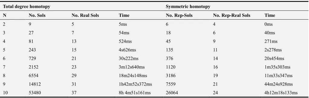
The Tables 1-4 show the details of solution for the discretized problem, which are obtained by using the total degree homotopy and symmetric homotopy. No. Sols refer to the numbers of solutions (including complex solutions) which increase exponentially with the numbers of eigenfunctions basis 9. No. Real Sols refer to the numbers of real solutions which are obtained by solving the target system of polynomial equations by the total degree homotopy. No. Rep-Sols and No. Real Rep-Sols refer to the numbers of representative solutions and the numbers of real representative solutions obtained by using symmetric homotopy, respectively.
Note that, such BVPs (29) may have infinitely many solutions [23], and the discretization problem has only finite solutions.
Table 1. The data of discretized problem (29) with cubic polynomial nonlinearity in 1 .
Total degree homotopy Symmetric homotopy
N No. Sols No. Real Sols Time No. Rep-Sols No. Rep-Real Sols Time
2 9 5 5ms 6 4 0ms
3 27 7 54ms 18 6 40ms
4 81 13 524ms 45 9 271ms
5 243 15 4s626ms 135 11 2s278ms
6 729 21 30s222ms 376 14 20s454ms
7 2152 23 3m12s640ms 1120 16 1m35s303ms
8 6554 29 18m24s148ms 3186 19 11m33s347ms
9 14812 31 1h42m52s372ms 7559 21 44m24s928ms
10 53480 37 8h 4m51s161ms 26064 24 4h12m18s133ms
The details of solution for discretized problem (29) are listed in Table 1. When 9 = 10, we observe that the number of solutions for total degree homotopy is approximately equal to 2 times the number of representative solutions, and the expected time by total degree homotopy is approximately equal to 2 times the expected time by symmetric homotopy.
5.2. Example 2
Consider the following variable-coefficient fourth-order ODE with an odd cubic polynomial nonlinearity
0 = 1 = 0 = 1 = 0, (30)
where = m − n and = m − n7 are chosen to be symmetric about the center of domain Ω.
Table 2 shows the details of solution for discretized problem (30). When 9 = 10, the number of solutions for total degree homotopy is approximately equal to 4 times the number of representative solutions, and the expected time by
total degree homotopy is approximately equal to 4 times the expected time by symmetric homotopy.
Due to the additional symmetry in the solution set of (30), we expect the efficiency of symmetric homotopy is more, comparing to solution of the problem with general cubic polynomial obtained in Table 1.
Table 2. The data of discretized problem (30) with an odd cubic polynomial nonlinearity in 1 .
Total degree homotopy Symmetric homotopy
N No. Sols No. Real Sols Time No. Rep-Sols No. Rep-Real Sols Time
2 9 5 16ms 4 3 0ms
3 27 7 31ms 10 4 15ms
4 81 9 203ms 25 5 47ms
5 243 11 1s406ms 70 6 406ms
6 728 13 10s672ms 194 6 3s516ms
7 2185 15 57s256ms 570 8 14s236ms
8 6561 17 5m50s672ms 1671 8 1m15s101ms
9 19672 19 33m53s536ms 4976 9 7m24s179ms
10 59024 20 2h15m43s774ms 14825 9 35m21s779ms
As previously mentioned, the number of solutions increases with the number of eigenfunctions basis 9. The solution set may contain spurious solutions, which means that approximation solution is not closed to original solutions for ODEs. Therefore, removing spurious solutions with certain filters will be necessary. The filtering strategy used in [11] can be a possible way to remove spurious solutions. The basic idea of this filter is based on error estimates of EEM, i.e., „ – &„†N≤ ,9f‡ , ‖ − &‖‰|≤ ,9f ‡X , where
&∈ 1& , ≥ 0 and , is a generic positive constant
independent of 9 . The approximate solutions & of
discretized problems on successively finer levels satisfy the error estimates, and then can be viewed as a solution path
; 9 parameterized by discretization level 9. Thus, the true approximate solutions should lie on a solution path. When 9 is large, the Cauchy's criterion for convergence implies that ‖ &− &X ‖ is very small. Applying Newton's method with initial guesses &= &f to the discretization system, one can expect convergence for nonspurious solutions.
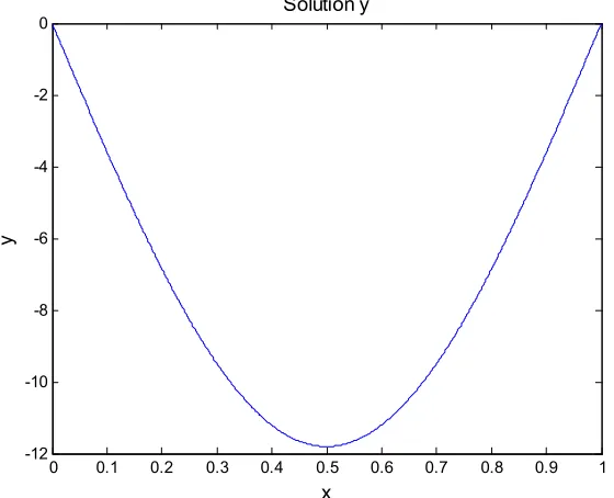
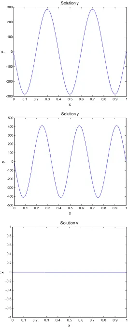
The representative solutions for discretized problem (30) after filtering with 9 = 20 are displayed in Figure 1.
0 0.1 0.2 0.3 0.4 0.5 0.6 0.7 0.8 0.9 1
-12 -10 -8 -6 -4 -2 0
x
y
0 0.1 0.2 0.3 0.4 0.5 0.6 0.7 0.8 0.9 1 -50
-40 -30 -20 -10 0 10 20 30 40 50
x
y
Solution y
0 0.1 0.2 0.3 0.4 0.5 0.6 0.7 0.8 0.9 1 -150
-100 -50 0 50 100 150
x
y
Solution y
0 0.1 0.2 0.3 0.4 0.5 0.6 0.7 0.8 0.9 1 -200
-150 -100 -50 0 50 100 150 200
x
y
Figure 1. The representative solutions for (30) after filtering with 9 = 20.
0 0.1 0.2 0.3 0.4 0.5 0.6 0.7 0.8 0.9 1 -300
-200 -100 0 100 200 300
x
y
Solution y
0 0.1 0.2 0.3 0.4 0.5 0.6 0.7 0.8 0.9 1 -500
-400 -300 -200 -100 0 100 200 300 400 500
x
y
Solution y
0 0.1 0.2 0.3 0.4 0.5 0.6 0.7 0.8 0.9 1 -1
-0.8 -0.6 -0.4 -0.2 0 0.2 0.4 0.6 0.8 1
x
y
5.3. Example 3
Consider the following variable-coefficient fourth-order ODE with quintic polynomial nonlinearity
− + = + [ [+ 7 7+ ~ ~, ∈ Ω ≡ 0, 1
0 = 1 = 0 = 1 = 0, (31)
where = = 7 = m − n and = [ = ~ = m − n7 are chosen to be symmetric about the center of domain Ω.
The details of solution for discretized problem (31) are listed in Table 3.
Table 3. The data of discretized problem (31) with quintic polynomial nonlinearity in 1‹.
Total degree homotopy Symmetric homotopy
N No. Sols No. Real Sols Time No. Rep-Sols No. Rep-Real Sols Time
2 25 7 31ms 15 5 16ms
3 125 9 735ms 75 7 515ms
4 625 15 13s892ms 325 10 7s547ms
5 3124 17 4m29s435ms 1622 12 2m15s30ms
6 15593 23 1h 2m 7s489ms 7853 15 28m52s373ms
7 77593 25 13h59m15s81ms 39112 17 6h51m5s51ms
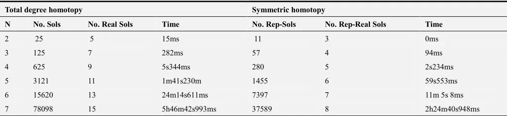
5.4. Example 4
Consider the following variable-coefficient fourth-order ODE with an odd quintic polynomial nonlinearity
− + = ~, ∈ Ω ≡ 0, 1
0 = 1 = 0 = 1 = 0, (32)
where = m − n and = m − n7 are chosen to be symmetric about the center of domain Ω.
Table 4. The data of discretized problem (32) with an odd quintic polynomial nonlinearity in 1‹.
Total degree homotopy Symmetric homotopy
N No. Sols No. Real Sols Time No. Rep-Sols No. Rep-Real Sols Time
2 25 5 15ms 11 3 0ms
3 125 7 282ms 57 4 94ms
4 625 9 5s344ms 280 5 2s234ms
5 3121 11 1m41s230m 1455 6 59s553ms
6 15620 13 24m14s611ms 7397 7 11m 5s 8ms
7 78098 15 5h46m42s993ms 37589 8 2h24m40s948ms
Table 4 shows the details of solution for discretized problem (32). When 9 = 7, the number of solutions for total degree homotopy is approximately equal to 2 times the number of representative solutions, and the expected time by total degree homotopy is approximately equal to 2 times the expected time by symmetric homotopy.
Similarly, because of the additional symmetry in the solution set of (32), the efficiency of symmetric homotopy is more, comparing to solution of the problem with general quintic polynomial obtained in Table 3.
0 0.1 0.2 0.3 0.4 0.5 0.6 0.7 0.8 0.9 1 -1
-0.8 -0.6 -0.4 -0.2 0 0.2 0.4 0.6 0.8 1
x
y
Solution y
0 0.1 0.2 0.3 0.4 0.5 0.6 0.7 0.8 0.9 1
-25 -20 -15 -10 -5 0 5 10 15 20 25
x
y
Solution y
0 0.1 0.2 0.3 0.4 0.5 0.6 0.7 0.8 0.9 1
-25 -20 -15 -10 -5 0 5 10 15 20 25
x
y
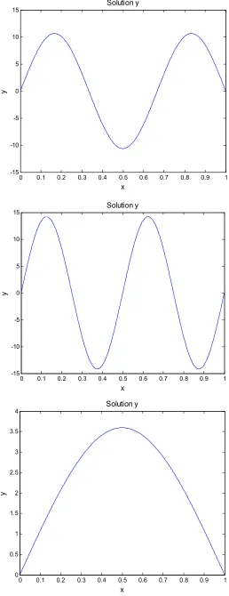
Figure 2. The representative solutions for (32) after filtering with 9 = 14.
0 0.1 0.2 0.3 0.4 0.5 0.6 0.7 0.8 0.9 1 -15
-10 -5 0 5 10 15
x
y
Solution y
0 0.1 0.2 0.3 0.4 0.5 0.6 0.7 0.8 0.9 1 -15
-10 -5 0 5 10 15
x
y
Solution y
0 0.1 0.2 0.3 0.4 0.5 0.6 0.7 0.8 0.9 1 0
0.5 1 1.5 2 2.5 3 3.5 4
x
y
6. Conclusion
In this paper, a numerical technique based on EEM is presented to obtain the approximate solutions for variable-coefficient fourth-order ODEs with (cubic/quintic) polynomial nonlinearity. We have extensively used the symmetry with dihedral group V which leads to simple computations. The symmetric homotopy constructed for solving discretization systems of ODEs can preserve the symmetry and reduce the computational cost. Numerical results demonstrated that the symmetric homotopy method is efficient and promising.
Acknowledgements
This work is supported in part by the National Natural Science Foundation of China (11571061, 11401075) and in part by the Fundamental Research Funds for the Central Universities (DUT16LK36).
References
[1] Z. Bai and H. Wang, On positive solutions of some nonlinear fourth-order beam equations, Journal of Mathematical Analysis and Applications, 270 (2002), pp. 357–368.
[2] Y. Yang, Fourth-order two-point boundary value problems, Proceedings of the American Mathematical Society, (1988), pp. 175–180.
[3] G. Bonanno and B. Di Bella, A boundary value problem for fourth-order elastic beam equations, Journal of Mathematical Analysis and Applications, 343 (2008), pp. 1166–1176.
[4] M. do Rosário Grossinho, L. Sanchez, and S. A. Tersian, On the solvability of a boundary value problem for a fourth-order ordinary differential equation, Applied Mathematics Letters, 18 (2005), pp. 439–444.
[5] L. Greenberg and M. Marletta, Numerical methods for higher order sturm-liouville problems, Journal of Computational and Applied Mathematics, 125 (2000), pp. 367–383.
[6] Z. S. Aliyev and F. M. Namazov, Spectral properties of a fourth-order eigenvalue problem with spectral parameter in the boundary conditions, Electronic Journal of Differential Equations, 2017 (2017), pp. 1–11.
[7] R. P. Agarwal, Boundary value problems for higher order differential equations, tech. report, 1979.
[8] G. Han and Z. Xu, Multiple solutions of some nonlinear fourth-order beam equations, Non-linear Analysis: Theory, Methods &Applications, 68 (2008), pp. 3646–3656.
[9] X. L. Liu and W. T. Li, Existence and multiplicity of solutions for fourth-order boundary value problems with three
parameters, Mathematical and Computer Modelling, 46 (2007), pp. 525–534.
[10] A. Cabada, R. Precup, L. Saavedra, and S. A. Tersian, Multiple positive solutions to a fourth-order boundary-value problem, Electronic Journal of Differential Equations, 2016 (2016), pp. 1–18.
[11] X. Zhang, J. Zhang, and B. Yu, Eigenfunction expansion method for multiple solutions of semilinear elliptic equations with polynomial nonlinearity, SIAM Journal on Numerical Analysis, 51 (2013), pp. 2680–2699.
[12] R. L. Burden and J. D. Faires, Numerical analysis, Cengage Learning, 2011.
[13] J. Alexander and J. A. Yorke, The homotopy continuation method: numerically implementable topological procedures, Transactions of the American Mathematical Society, 242 (1978), pp. 271–284.
[14] T. Y. Li, Numerical solution of multivariate polynomial systems by homotopy continuation methods, Acta numerica, 6 (1997), pp. 399 436.
[15] T. Y. Li, Numerical solution of polynomial systems by homotopy continuation methods, Handbook of numerical analysis, 11 (2003), pp. 209–304.
[16] J. Verschelde, Algorithm 795: Phcpack: A general-purpose solver for polynomial systems by homotopy continuation, ACM Transactions on Mathematical Software (TOMS), 25 (1999), pp. 251–276.
[17] T. L. Lee, T. Y. Li, and C. H. Tsai, Hom4ps-2.0: a software package for solving polynomial systems by the polyhedral homotopy continuation method, Computing, 83 (2008), pp. 109–133.
[18] D. J. Bates, J. D. Hauenstein, A. J. Sommese, and C. W. Wampler, Bertini: Software for numerical algebraic geometry (2006), Software available at http://bertini. nd. edu.
[19] A. J. Sommese and C. W. Wampler II, The Numerical solution of systems of polynomials arising in engineering and science, World Scientific, 2005.
[20] E. L. Allgower, D. J. Bates, A. J. Sommese, and C. W. Wampler, Solution of polynomial systems derived from differential equations, Computing, 76 (2006), pp. 1–10. [21] X. Zhang, J. Zhang, and B. Yu, Symmetric homotopy method
for discretized elliptic equations with cubic and quantic nonlinearities, Journal of Scientific Computing, 70 (2017), pp. 1316–1335.
[22] W. Hao, J. D. Hauenstein, B. Hu, and A. J. Sommese, A bootstrapping approach for computing multiple solutions of differential equations, Journal of Computational and Applied Mathematics, 258 (2014), pp. 181–190.