in the population sciences published by the Max Planck Institute for Demographic Research Konrad-Zuse Str. 1, D-18057 Rostock · GERMANY www.demographic-research.org
DEMOGRAPHIC RESEARCH
VOLUME 23, ARTICLE 29, PAGES 807-846
PUBLISHED 29 OCTOBER 2010
http://www.demographic-research.org/Volumes/Vol23/29/ DOI: 10.4054/DemRes.2010.23.29
Research Article
The impact of unemployment on the
transition to parenthood
Berkay Özcan
Karl Ulrich Mayer
Joerg Luedicke
©2010 Berkay Özcan, Karl Ulrich Mayer & Joerg Luedicke.
This open-access work is published under the terms of the Creative Commons Attribution NonCommercial License 2.0 Germany, which permits use, reproduction & distribution in any medium for non-commercial purposes, provided the original author(s) and source are given credit.
1 Introduction 808
2 Theoretical background 812
3 Data and methods 817
3.1 Data and sample 817
3.2 Model specification and variables 821
4 Results 824
4.1 Results for women 824
4.2 Results for men 828
4.3 Interaction effects 830
4.4 Additional specifications and sensitivity analysis 834
4.4.1 Period-specific effects 834
4.4.2 Sensitivity check for timing of conception 836
5 Discussion and conclusions 837
6 Acknowledgements 840
The impact of unemployment on the transition to parenthood
Berkay Özcan1
Karl Ulrich Mayer2
Joerg Luedicke3
Abstract
This paper seeks to advance our understanding about the impact of unemployment on fertility. From a theoretical perspective, both negative and positive effects might be expected. Existing empirical studies have produced contradictory results, partly because of varying institutional contexts, the use of different measures, and left-censoring problems. We address these theoretical and methodological problems in the extant literature. Our data comes from the German Life History Study (GLHS) and, in particular, the data on the 1971 cohort, which was collected in two representative and retrospective surveys conducted in East and West Germany in 1996-1998 and 2005. Using monthly information, we perform event history analysis to identify the timing of fertility for both men and women conditional on a number of covariates. We present our results as a comparison between East and West Germany, as the institutional contexts, the labour markets, and the value systems differ considerably between the two parts of the German state.
1. Introduction
The empirical relationship between unemployment and fertility is hardly uncharted territory. Specifically, many studies have investigated the negative correlation between the trends in women’s employment and fertility up to the 1990s (see Budig 2003 and Brewster and Rindfuss 2000 for a review of the earlier literature). Recently, however, a number of researchers have noted that the sign of the cross-country correlation coefficient has flipped (Adsera 2004, Adsera 2005, Ahn and Mira 2002, Brewster and Rindfuss 2000, Esping-Andersen 1999, Esping-Andersen 2009, Engelhardt and Prskawetz 2004). These studies showed that, since the late 1980s, countries with lower rates of female employment also experienced lower rates of fertility. In addition, the studies found that the downward trends in fertility coincided with heightened unemployment for women. Thus, the positive cross-country correlation between fertility and female labor force participation was often attributed to extended durations of high unemployment (e.g., Adsera 2002, Engelhardt and Prskawetz 2004, Ahn and Mira 2002).
Although the studies above successfully identified a relationship between unemployment and total fertility rates, for a number of reasons they did not adequately unravel the mechanisms through which unemployment influences parenthood transitions. First, they usually used aggregate fertility data, which are particularly vulnerable to temporary fluctuations in the age at first marriage and/or first birth (Adsera 2005). Second, the effects of unemployment and its duration might vary due to factors that are difficult to capture at the aggregate level, such as an individual’s education, age and partnering structure. Third, changes in the aggregate unemployment rate can affect individual behavior either by altering the risk perception of individuals or by depressing average wage levels in the society (Kravdal 2002), either of which might affect fertility. In other words, aggregate unemployment may affect fertility behavior indirectly, even if an individual does not experience unemployment herself. Finally, the theoretical arguments presented in these studies have ambiguous predictions regarding the direction of the impact. Hence, testing these predictions requires individual-level data.
Rindfuss, Morgan, and Swicegood 1988).4 However, the results of these studies are
contradictory and far from conclusive. One set of findings reported no effect of unemployment on the fertility behavior of women in various national studies, including Germany (Kreyenfeld 2009), Norway (Kravdal 2002), the U.S. (Rindfuss et al. 1988), and Russia during the transition period (1994-1996) (Kohler and Kohler 2002). Some even found a positive impact for women with low levels of education (Kreyenfeld 2009, Hoem 2000). Another set of findings suggested, however, that unemployment has a negative effect on the transition to motherhood. For example, Hoem (2000) found that the overall impact of unemployment is negative. Using European Community Household Panel (ECHP) data, Adsera (2005) also found negative effects for 15 European countries, and Gonzalez and Jurado-Guerrero (2006) found negative effects for Italy, Spain, and France. The few studies that have analyzed the relationship between men’s fertility behavior and unemployment also reported contradictory findings (e.g., Tölke and Diewald 2002, Sullivan and Falkingham 1991, Kravdal 2002).
In addition to the ambiguity in the theoretical arguments (which is discussed in the next section), our decision to conduct this research was motivated by our concerns about a number of methodological shortcomings in the extant literature, which may explain the variations in the findings.
First, due to data limitations, the existing literature is plagued by left-censoring problems. The studies that used panel data often chose a reasonable sample size over a sample without left-censoring. As a result, most analyses were applied to samples that are likely to have systematically selected certain types of women.For example, women in the same age range, but who made the transition to motherhood before the panel started, and women not living with their children at the time of the interview, were excluded (Kreyenfeld 2009; Kravdal 2002; Gonzalez and Jurado-Guerrero 2006;
Adsera 2005; Schmitt 2008).5 Since neither the number of excluded women nor their
unemployment experiences is known, it is hard to generalize these findings.
Second, women’s relationship histories have frequently been either crudely measured through, for example, the use of a binary variable for the presence of a partner (Kreyenfeld 2009); or their histories were ignored completely (Kurz 2005;
4 There is also a large body of literature that focuses on the link between women’s work behavior (i.e.,
employment) and fertility (literature summarized in Brewster and Rindfuss 2000 and Budig 2003), in which the reference category is often non-employment instead of unemployment. The non-employment category groups all types of women who are outside the labor market for various reasons, and is therefore fundamentally different from unemployment.
5 Gonzalez and Jurado-Guerrero (2006), and especially Adsera (2005), attempted, although imperfectly, to
Hoem 2000; Kravdal 2002,6 Adsera 2005). Where a detailed partnership history that
distinguished between marriage and cohabitation was taken into account, no additional attempts were made to include partner characteristics (Tölke and Diewald 2003). In fact, to our knowledge only two studies incorporated any partner characteristics into their models: Kohler and Kohler (2002) incorporated the partner’s employment status, and Gonzalez and Jurado-Guerrero (2006) included the partner’s income. This absence is regrettable, because there are several theoretical reasons for including partner characteristics (Corijn, Liefbroer, and Gierveld 1996), which we will discuss in the next section.
Third, studies using individual-level data have also frequently been limited in their independent variables. For example, unemployment was sometimes measured yearly (or via imputed data) (e.g., Tölke and Diewald 2003), or it was proxied by another variable, such as the “annual unemployment benefits” of low-income earners (e.g., Hoem 2000). Meanwhile, in other studies unemployment was only measured for a short period due to incomplete work histories (Kravdal 2002). These limitations may have also contributed to the variations in the findings.
Finally, the data sources used and time periods covered differed considerably between studies. The same can be said for the institutional structures and labor market trends. These differences may also be responsible for the contradictory findings in the literature. If this is true, however, country selection becomes crucial. For example, some of the countries analyzed previously, such as Norway and the U.S., did not—until very recently—experience unemployment levels that were as high or as sustained as the levels seen in Central and Southern European countries. Moreover, the decline in the fertility rate in Norway and the U.S. was not as dramatic. In these cases, as Kravdal (2002) reminded us, we should be cautious when interpreting the absence of an impact of unemployment on fertility behavior.
Another consequence of country selection relates to differing unemployment benefits. Countries have varying degrees of compensation, which further complicates the comparison of findings.
In the present study, we have been able to overcome many of these methodological issues. First, we do not limit our sample to only women or men; rather, we conduct separate analyses for each. Second, we observe each individual from age 16 onwards, and thus avoid left-censoring problems. Third, because we have the complete birth history of individuals, we do not exclude the birth of any children outside the household, as many previous studies have done. Fourth, we include a fine-grained
6 In fact, Kravdal (2002) discusses in detail the role of relationship types and partner information. But he then
partnership history that distinguishes between several types of relationship status—i.e., single, in a non-residential relationship, cohabitating, or married—and includes the partner’s age and education. Fifth, we use detailed monthly data to follow individuals’ employment and relationship histories up to their first birth, including all periods of employment and unemployment, as well as activity outside the labor market.
Last but not least, our study compares East and West Germany, which proves to be especially useful for a number of reasons. First, the two parts of Germany have identical unemployment compensation schemes, so the impact of unemployment in the regions should not vary due to differences in the relative generosity of unemployment benefits. Despite this similarity, levels of unemployment and economic instability were (and are) much higher in East Germany (Mayer and Schulze 2009:29, 91-96, 140-148). Additionally, median ages at first marriage and first birth have increased in West Germany for more than three decades, and in East Germany since 1991. According to period data, the overall median age at marital first birth in Germany reached its lowest point in 1970, at age 24, and has since risen beyond age 29. By 2006, period fertility converged between East and West Germany (Dorbritz 2008, Tivig and Hetze 2007).
Institutional backgrounds and values concerning fertility also remain strikingly different in East and West Germany. For example, even though family policy incentives for marriage and first births were curtailed in East Germany after unification, childcare facilities continued to be much better than those in West Germany (Trappe 2006). Compared to their West German counterparts, East German women spend fewer years in school, have higher rates of labor force participation, and view the combination of work and motherhood as less problematic (Statistisches Bundesamt 2006: 523; Mayer and Schulze 2009: ch.5). East German women, who are more accustomed to economic scarcity and cramped housing conditions, were exposed to a sudden increase in consumption options after 1989. Since the 1970s, East German women have had a “culture” of early births, with or without marriage, and a very low rate of childlessness (Huinink and Kreyenfeld 2006; Bernardi et al. 2007; Trappe and Sorensen 1995). Although problems of unemployment also affected West German women, these problems were especially severe for East German women after unification (Diewald 2006; Trappe 2004). Finally, the two German sub-societies are characterized by different scales and structures of social inequality. East Germany was (and partly still is) a more egalitarian, homogeneous society with fewer class barriers, whereas West Germany has a pronounced class structure based on its education and training systems.
the person’s gender, the person’s education, the partner’s education (for men), and the institutional settings (contexts) in each region. We do not find evidence of a differential impact of unemployment across the life-cycle. We also do not find evidence of a negative impact of unemployment for men, as has been suggested by the neoclassical theory of fertility. Overall, we find that many predictions of the neoclassical theory of fertility are not supported by our data.
The rest of the paper is organized as follows. In Section 2, we offer a brief summary of competing theories, from which we formulate our hypotheses. In Section 3, we describe our data and sample and discuss the construction of our main covariates. In Section 4, we present our results in three subsections: first for men, then for women, and then the results of models, which include interaction effects between our main explanatory variables. Section 4 also tests for additional specifications and period-specific effects, and reports a number of robustness checks. The paper ends with a discussion and conclusion in Section 5.
2. Theoretical background
How does an individual’s experience of unemployment influence his or her transition to parenthood? Most theoretical accounts of fertility decisions rely on the neoclassical economic model of fertility developed by Becker (1981) and its extensions. The following arguments are, albeit in a synthesized manner, based on the discussions regarding those extensions outlined in Kravdal (2002), Kohler and Kohler (2002), Bernardi et al. (2008), and Adsera (2004).
Before explaining their main predictions, it is important to note that neoclassical fertility models are based on a number of important assumptions. They assume that children are costly both in economic and in social terms, and that they necessitate investments of time that are especially high for the months immediately following the birth. Most studies that test the predictions of the neoclassical model also assume that traditional gender roles are common and persistent even in advanced societies (see the critique of this in Esping-Andersen 2009). This assumption dictated that researchers only consider women’s time for childbearing and rearing, especially around the first birth. Because men’s time investments are considered irrelevant, the neoclassical model predicts that unemployment will have different effects on the fertility of men and women.
For men, the prediction is negative and directly related to unemployment’s effect on income. According to this model, unemployment leads to a decline in income that reduces household resources, and thus lessens the likelihood of becoming a father; this
income effect, sociological models also argue that (from the woman’s perspective) unemployment may make a man appear to be less reliable as a potential father, or to be a less favorable candidate for family formation in general (Kravdal 2002).
For women, however, the neoclassical model predicts two opposing effects. The first is an income effect that reduces total household income, and hence suggests a negative outcome, analogous to the effect for men. But for women, a sizable decrease in earnings also reduces the opportunity cost of spending time caring for children; this is known as the substitution effect. (Recall that the underlying assumption is that only the mother’s time is required for child-related activities). As a result, the aggregate effect for women depends on whether the income effect or the substitution effect dominates.
Substitution effects can be assumed to be stronger for first births because there is a general social norm against remaining childless (Kravdal 2002; Konietzka and Kreyenfeld 2007). This theoretical background leads us to:
Hypothesis 1: For men, unemployment will delay the transition to fatherhood. For women, unemployment will have no clear effect due to the opposing income and substitution effects.
But the impact of unemployment might also be contingent upon expectations concerning its duration. Different theoretical models make contradictory predictions regarding the effect of unemployment duration. Adsera (2004) claims that a temporary period of unemployment can be perceived as “a cheap time to have children.” Yet if unemployment becomes persistent, then pregnancy might imply “a weaker commitment to labor market,” especially if it happens early in the life course. As a result, childbearing at younger ages, combined with longer periods of unemployment, might turn into “an unemployment trap,” and lead to a considerable loss of lifetime income (p.22). In sum, this interpretation predicts that the expectation of a short unemployment spell might have no impact or a positive impact, whereas the expectation that the period of unemployment will be long or persistent should have a negative impact. Because this prediction refers to (the time costs of) motherhood, we believe that it better explains women’s than men’s behavior.
breadwinner role is still dominant in most advanced societies. Consequently, the two contrasting interpretations lead to our second hypothesis:
Hypothesis 2a: Each additional month of unemployment delays the transition to motherhood.7
Hypothesis 2b: Each additional month of unemployment delays the transition to fatherhood, but this effect disappears in the long run.
Hypothesis 2c: For women, this negative effect of each additional month of unemployment will disappear at later ages.
In fact, the “substitution effect” in neoclassical fertility models makes sense only if we also make certain assumptions about expectations regarding the unemployment duration. Since the time span from conception through to early infancy is 12 to 15 months, expectations about the duration of unemployment must logically coincide with this period for the substitution effect to be meaningful (Kravdal 2002). In other words, women would only decide to have a child during unemployment if they assume the period of joblessness will last at least 12 months. If they expect to be unemployed for less than a year, they may be more likely to delay pregnancy. Alternatively, unemployment might cause women to lower their career aspirations—in line with sociological arguments about the erosion of self-confidence during unemployment— and be willing to accept lower-quality jobs from unemployment. For these women, the alternate track of motherhood might allow them to adopt a role that is highly valued among peers, and within the marital dyad (Friedman, Hechter, and Kanazawa 1994).
These mechanisms may operate differently, however, depending on a woman’s educational attainment. Let us consider, for example, the contradictory effects of unemployment for highly educated women. On the one hand, extended durations of unemployment might suggest an especially high income loss (i.e., stronger income effect) for these women, and thus imply a delay in fertility. On the other hand, highly educated women might also have more resources to offset the negative income effect of unemployment. Consequently, unemployment may provide an opportunity to take time off, which would otherwise be more costly to take than for a woman with a low level of schooling. In other words, the overall impact of unemployment for highly educated women depends on the strength of the net “income effect,” which may be a function of
7 This variable measures cumulative unemployment experience and it should be thought as a proxy for
both the wage distribution and costs of childrearing. We can thus formulate our third hypothesis:
Hypothesis 3: Unemployment will accelerate the transition to motherhood for less-educated women in East and West Germany, and for highly educated women in East Germany.
Until now, following the neoclassical theory of fertility, we have implicitly assumed a household (e.g., unitary) model with a single decision maker. We have also assumed that only the decision maker’s income determines the resources available for childrearing. Furthermore, we pointed out the two underlying assumptions of this model that shaped theoretical arguments about the impact of unemployment: the prevalence of the male breadwinner and the irrelevancy of men’s time for childrearing activities. In fact, both of these assumptions can be challenged and relaxed. For example, Esping-Andersen (2007, 2009) and Brodmann, Esping-Esping-Andersen, and Güell (2007) provide evidence that, in societies with higher levels of gender symmetry, such as Denmark, men’s potential childrearing time also affect fertility decisions.
Recent evidence of increasing gender symmetry suggests that we should move away from the model of unitary household decision-making, and towards a more flexible, joint decision-making framework. Consequently, the within-household bargaining process and the relative endowments of each spouse become crucial in determining the impact of unemployment and job stability on childbearing decisions. In other words, it is not just an individual’s, but also his/her partner’s preferences and characteristics that can substantially alter the impact of income and substitution effects (Corijn et al. 1996).
be stronger. This is, of course, contingent on her own education level, and on her husband being employed. In any case, when an unemployed woman is married, the effect differs from when she is single, because the income effect may be alleviated by her husband’s income.
To capture and test variations in the theoretical arguments due to the partner’s education, we formulate the following hypotheses:
Hypothesis 4a: Having a highly educated partner will delay an unemployed man’s transition to fatherhood.
Hypothesis 4b: Having a highly educated partner will accelerate an unemployed woman’s transition to motherhood.
The degree of gender symmetry in decision-making can be a function of values and social norms regarding family and children. It can also be reflected in institutional structures, which may play crucial roles in mediating the impact of unemployment on parenthood decisions. For example, Rindfuss et al. (1996) and Esping-Andersen (1999, 2009) have persuasively argued that women have more children, and have them earlier, in settings where high rates of female employment and gender symmetry prevail, such as the Scandinavian countries, the United Kingdom, and the United States; and where favorable conditions exist for combining work and family obligations, such as (universal) childcare and paternity leave. Many studies of Southern Europe, particularly of Italy and Spain, have identified a lack of these institutions as the primary reason for low fertility (Gonzalez and Jurado-Guerrero 2006; Adsera 2005; Esping-Andersen 2007). These studies show that women who are in the top household income quartile, and women who are out of the labor force, have the highest fertility, which indicates that working women are faced with a tradeoff between career and motherhood. In societies in which gender symmetry is low and institutions do not facilitate the combination of these two roles, the time advantage of unemployment is especially limited for highly educated (career-oriented) women and for all women during the initial stages of their careers. This suggests that women in different social and institutional settings may react differently to unemployment in making fertility decisions.
The comparison between East and West Germany provides special opportunities to
test these theoretical propositions. Since unemployment and economic uncertainties
differences between East and West Germany might explain the higher and earlier fertility in the East? First, childcare facilities are still much better in the East, and it continues to be easier to combine full-time employment and having children in the East than in the West (Büchel and Spiess 2002). Second, East German women, unlike West German women, do not believe that it is harmful to very small children for their mother to work (Mayer and Schulze 2009: 188). Therefore, they should feel less encouraged to use periods of unemployment as opportunities for staying at home (Mayer and Schulze 2009: 184-188). Third, marriage is not a prerequisite for parenthood in the East to the extent that it is in the West; therefore, the economic preconditions of weddings and marriage should have less impact in the East. Fourth, the level of employment and full-time employment is higher in the East, and the share of wives’ earnings in household income is also higher (Mayer and Schulze 2009: 147, 151). The division of work and household responsibilities in East Germany more closely resembles the egalitarian work-family balance typical of Scandinavian countries than the male breadwinner model that remains prevalent in West Germany. While greater economic instability should delay and dampen fertility in the East, this might be (at least partially) offset by lower income effects due to better childcare and the higher labor force commitment of women. We will discuss the role of these contextual differences and similarities in detail in Section 5.
3. Data and methods
3.1 Data and sample
We use German Life History Study (GLHS) 1971 cohort data for the analysis (Matthes, Lichtwardt, and Mayer 2004; Hillmert and Mayer 2004; Matthes 2005; Mayer 2008). The GLHS 1971 cohort includes individuals in East and West Germany who were born in 1971. This cohort is uniquely interesting because its members were 18 years old when the Berlin Wall came down in 1989. They thus transitioned to adulthood under the new conditions of unified Germany, even though most of their cultural upbringing and non-post-secondary education took place under the two different regimes. Members of this cohort also experienced different sets of family policies. The attitudes of the women of this cohort towards family formation differ significantly between East and West, even as family policies, consumption patterns, and labor market regulations became increasingly similar in the regions.
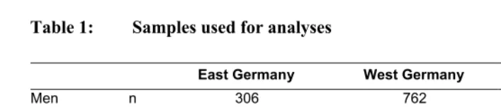
the sizes of samples used in East and West Germany by gender. The total sample used here contains 1,068 complete life histories of men and 936 complete life histories of women. Events and transitions were recorded forward in time and dated monthly.
Table 1: Samples used for analyses
East Germany West Germany Total
Men n 306 762 1068
% 28.7 71.3 100
Women n 286 650 936
% 30.6 69.4 100
Note: The numbers above indicate number of individuals (not spells).
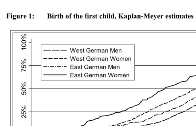
As noted above, an important advantage of our data is that it avoids the left-censoring problem which is pervasive in the extant research (e.g., Kreyenfeld 2009; Gonzalez and Jurado-Guerrero 2006; Schmitt 2008). We follow all respondents from the age 16 (the onset of fertility risk) until they make their transition to parenthood, or until the last interview date (at approximately age 348) (See Figure 1).
We exclude unusual transitions to parenthood (e.g., adoptions or step-parenthood via marriages) from our sample, since the decision-making process during
unemployment is too complex to model.9 However, it should be noted that Table 2
shows that East German men are more than twice as likely to adopt a child as their West German counterparts. The relevant question here is whether employment instability is correlated with becoming a stepfather. In other words, our estimates might be slightly biased in East Germany if the characteristics that make men likely to enter parenthood via adoption and step-fatherhood also affect their employment status. However, we believe it is unlikely that such characteristics exist specifically for step-fatherhood.
8 This can be considered a limitation because the observation window is shorter than the possible fertility
window of women, and it ends at the same age for men, which may be especially problematic for the highly educated.
9 This is a common practice in the literature, although to our knowledge none of the papers we cite here in
Figure 1: Birth of the first child, Kaplan-Meyer estimates
0%
25
%
50
%
75
%
10
0%
20 25 30 35
Age (in years) West German Men
West German Women East German Men East German Women
Table 2: Nature of the relationship between parents and their first child
Relationship to first child
Own child Adopted child Child of partner
East Germany Men 82.4 17.6 0.0
Women 100.0 0.0 0.0
Total 92.1 7.9 0.0
West Germany Men 91.4 7.5 1.1
Women 98.8 1.2 0.0
Total 95.7 3.9 0.5
Note: The percentages above are for the respondents at the age of 34 or at the age of childbirth .
and West Germany. Looking at gender, we observe that slightly more women than men are in education and are inactive. Except for these differences, our samples have rather similar distributions in the two regions.
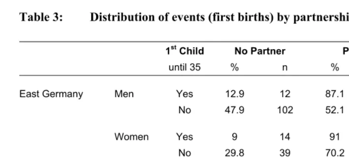
Table 3: Distribution of events (first births) by partnership status
1st Child No Partner Partner Total
until 35 % n % n n
East Germany Men Yes 12.9 12 87.1 81 93
No 47.9 102 52.1 111 213
Women Yes 9 14 91 141 155
No 29.8 39 70.2 92 131
West Germany Men Yes 8.2 19 91.8 213 232
No 46.6 247 53.4 283 530
Women Yes 8.1 26 91.9 295 321
No 37.1 122 62.9 207 329
Table 4: Employment status (person-spell data)
Status
Employed Unemployed Education Inactive n
East Germany Men 49.0 8.0 32.0 11.0 3504
Women 43.9 7.5 44.7 3.9 2843
West Germany Men 46.2 4.8 38.3 10.7 8716
Women 47.7 3.5 43.6 5.2 6764
Note: The figures above indicate the percentages of the corresponding person-spells, not of the individuals. Because we adopt a
3.2 Model specification and variables
We use an event history analysis (e.g., Blossfeld and Rohwer 1995) that allows us to examine transitions to parenthood, and that controls for right-censored data. The crucial statistical concept here is conditional likelihood, i.e., a hazard rate: it is simply the likelihood that an event will take place within a time interval, conditional on it having not occurred previously. In our case, we apply a piecewise constant exponential model, because it relaxes assumptionsabout the functional form of the hazard rates by allowing the hazard to vary between specified portions of time within our observation window. The piecewise constant exponential model can be depicted as follows:
) ' exp(
)
( ip i i
i t X
r = α +β if t Єp
where the subscript p denotes a specific sub-period—in this, the age group10 (<20, 20– 25, 25-30 or >30 years old, respectively)—and X represents a vector of explanatory and control variables used in the analysis. αip is a constant coefficient associated with the time period p. Finally, subscript i denotes the transition rate from origin to destination state. Thus, our main coefficient estimates (βp) reveal information regarding the hazard
rate at different points in time. Our dependent variable is the timing (age) at the first birth. Thus, for example, in isolation a positive coefficient implies that the hazard is increasing, which in turn means transitions occur at earlier ages (faster). We subtract nine months from the date of the first birth in order to capture the time at which the decision for parenthood was made, and avoid reverse causation problems. In other words, our dependent variable is the age at conception (of the first live birth).11
We have a number of time-varying explanatory variables which measure different
aspects of career and economic uncertainty. Our first direct measure is employment
status, which is a categorical time-varying variable that indicates four different states: employed, enrolled in secondary and tertiary education, unemployed, or inactive. Our
second measure of career and economic uncertainty is the number of months spent in
unemployment, i.e., unemployment duration. This is a cumulative count of months in all unemployment spells. This variable indicates the total loss of human capital in the form
10 Because we have only one cohort (1971), period effects should be identical to the age effects. It is not
exactly identical because we have a variation of a few months among the members of the cohort, although this discrepancy does not affect the results.
11 Of course the decision to conceive is not the same thing as conception. We discuss this in detail in Section
of labor market experience due to unemployment. We also generated a variable that counts the number ofunemployment spells.12
We measure respondents’ educational attainment in two ways. First, we take into account each respondent’s educational level. It is important to note that the East and West Germans in this cohort experienced two different school systems. In West Germany, there are three main branches of schooling which diverge after the fourth
grade. Hauptschule is an eight-year track which qualifies students for basic
apprenticeships and vocational training in certain occupations. A higher degree (Mittlere Reife) is awarded upon graduation from Realschule, a 10-year track that prepares pupils for a wider range of vocational training programs. The highest degree is the Abitur, which is earned following attendance at Gymnasium, and requires a total of 12 or 13 (depending on the region) years of schooling. Only students who have received the Abitur degree are permitted to attend university. In contrast, in the former GDR,
there was one type of school, Polytechnische Oberschule (POS), which nearly all
students attended from the first through the 10th grades. The students then received a degree which qualified them to begin an apprenticeship. However, to gain entry to university, students from the former GDR also had to earn the Abitur, which required them to attend Erweiterte Oberschule (EOS), a two-year extension of the POS.
To create a comparable measure of education between the East and West, we constructed a variable with three categories. We distinguish between the low-educated,
i.e., individuals whose highest degree is the Hauptschulabschluss in West Germany, or
who left POS after the eighth grade in East Germany; the medium-educated, i.e.,
individuals who graduated from school after 10th grade; and the highly educated, i.e., individuals who were qualified to enter university. The distribution of these categories in East and West Germany is shown in Table 5. There are striking differences in the distribution of people across these categories in East and West Germany. There is almost no one in the lowest education category in East Germany, and the percentage of people in the highest educational category in West Germany is almost double the respective percentage in East Germany. These differences are not an artifact of our categorization, but instead reflect real differences in the two parts of the country (see Mayer and Schulze 2009 for details of the education structures of East and West Germany).
Our second measure of educational attainment captures the amount of time spent in secondary and tertiary education. More precisely, it counts the months spent in secondary and post secondary education since age 16. This variable can also be seen as
12 This variable is highly correlated with the number of months of unemployment (approximately r =0.7)
a proxy for age at labor market entry, which matters for our study since people often delay parenthood until they enter the labor market (Huinink and Mayer 1995; Kreyenfeld 2006).
Since the timing of birth and the timing of marriage are usually linked, and marriage accelerates the timing of the first birth (Blossfeld and Huinink 1991), it is important to control for marital status (Blossfeld and Rohwer 1995). As described above, our partnership status variable has four categories: no partner, a non-cohabitating partner, a non-cohabitating partner, or a spouse. We also control for the partner’s age and use the partner’s educational level as an indicator of the partner’s human capital to allow for testing of Hypothesis 4. Finally, we constructed a control variable that counts the number of prior job shifts,13 which is used to distinguish instability induced by job changes from dramatic changes in earnings induced by unemployment spells.
Table 5: Level of education
School degree
Low Middle High
East Germany Men 5.2 73.2 21.6
Women 4.2 73.4 22.4
West Germany Men 30.4 27.7 41.9
Women 22.6 35.6 41.8
Note: These figures indicate the percentages of all individuals.
13 It may be expected that the number of months spent in unemployment would also be correlated with the
4. Results
The last six tables (Tables 6 to 11) display the results of our analysis. We ran separate models for women and men, which we outline in Sections 4.1 and 4.2, respectively. We also report separate sets of models for East and West Germany. Our aim at this stage is to define a saturated model of fertility timing, and to analyze the effects of unemployment and partnership status. In Section 4.3, we use the saturated model defined in Sections 4.1 and 4.2 as a “baseline,” and then introduce a number of interaction effects. Because our focus in Section 4.3 is only on the interaction effects, the variables of the baseline saturated model will be considered solely for control reasons. Finally, we discuss additional specifications and sensitivity checks in Section 4.4.
4.1 Results for women
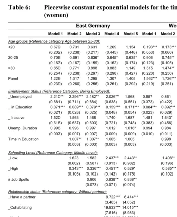
Table 6 shows the results for transition to motherhood in East and West Germany. We report five different specifications per country. We set the age group 25-30 as the reference category in all models. All the coefficients in Tables 6 to 11 represent hazard ratios. Our analytical strategy is to begin with a simple model (Model 1), and then to add sets of covariates and controls stepwise in each specification from Models 2 to 5.
Model 1 includes two time-varying covariates to capture the unconditional effects
of unemployment; unemployed is one of the three dummy variables of our
Table 6: Piecewise constant exponential models for the timing of the first birth (women)
East Germany West Germany
Model 1 Model 2 Model 3 Model 4 Model 5 Model 1 Model 2 Model 3 Model 4 Model 5
Age groups (Reference category Age between 25-30):
<20 0.679 0.731 0.631 1.269 1.154 0.193*** 0.173*** 0.181*** 0.569* 0.470**
(0.202) (0.238) (0.217) (0.445) (0.446) (0.053) (0.060) (0.063) (0.189) (0.158)
20-25 0.706 0.691 0.636* 0.645* 0.635* 0.906 0.745** 0.766* 0.990 0.814
(0.163) (0.167) (0.159) (0.162) (0.174) (0.123) (0.105) (0.111) (0.143) (0.125)
>30 0.850 0.771 0.898 0.883 1.149 1.315 1.474** 1.404* 1.402* 1.841***
(0.254) (0.238) (0.297) (0.298) (0.427) (0.220) (0.250) (0.253) (0.250) (0.364)
Panel 1.229 1.317 1.295 1.307 1.405 1.562*** 1.726*** 1.714*** 1.336** 1.350**
(0.239) (0.260) (0.256) (0.261) (0.292) (0.219) (0.251) (0.249) (0.196) (0.203)
Employment Status (Reference Category: Being Employed):
_Unemployed 2.210** 2.296*** 2.182** 2.026** 1.568 0.857 0.861 0.877 0.968 0.921
(0.681) (0.711) (0.684) (0.638) (0.551) (0.373) (0.422) (0.428) (0.453) (0.426)
_ in Education 0.071*** 0.089*** 0.079*** 0.159*** 0.171*** 0.084*** 0.092*** 0.096*** 0.216*** 0.181***
(0.021) (0.026) (0.025) (0.048) (0.054) (0.023) (0.029) (0.031) (0.066) (0.058)
_ Inactive 1.520 1.563 1.468 1.740 1.687 1.481 1.643* 1.689* 1.558 1.697*
(0.616) (0.637) (0.603) (0.721) (0.748) (0.383) (0.456) (0.472) (0.436) (0.480)
Unemp. Duration 0.996 0.996 0.997 1.012 1.016* 0.994 0.984 0.983 0.981* 0.989
(0.007) (0.007) (0.007) (0.009) (0.009) (0.010) (0.011) (0.011) (0.011) (0.012)
Time in Education 1.007** 1.007** 1.005 1.005 0.998 0.998 1.001 1.001
(0.003) (0.003) (0.003) (0.003) (0.003) (0.003) (0.002) (0.003)
Schooling Level (Reference Category: Middle Level):
_Low 1.623 1.582 2.437** 2.443** 1.408** 1.409** 1.626*** 1.562***
(0.602) (0.587) (0.913) (0.982) (0.196) (0.196) (0.229) (0.225)
_High 0.343*** 0.336*** 0.451** 0.529* 0.585*** 0.590*** 0.600*** 0.619**
(0.105) (0.102) (0.142) (0.175) (0.102) (0.103) (0.108) (0.119)
# Job Spells 0.906 0.838** 0.838** 1.039 1.020 1.022
(0.073) (0.071) (0.074) (0.047) (0.049) (0.052)
Relationship status (Reference category: Without partner):
_Have a partner 9.722*** 6.414*** 3.014*** 5.027***
(3.405) (4.052) (0.896) (2.697)
_Cohabitating 19.933*** 14.015*** 9.129*** 15.745***
(7.516) (8.983) (2.621) (8.278)
_Marriage 35.114*** 24.679*** 32.318*** 54.827***
(14.412) (15.545) (8.967) (28.637)
Age of Partner 1.098* 1.029
(0.055) (0.038)
Age-Squared of Partner 0.998* 0.999*
(0.001) (0.001)
Partner Human Capital 0.876 0.969
(0.073) (0.037)
Log likelihood -120.762 -112.765 -112.008 -52.558 -50.968 -190.610 -157.443 -157.090 18.336 26.904
Chi-Squared 283.33*** 299.33*** 300.84*** 419.74*** 390.63*** 755.79*** 786.75*** 787.46*** 1138.31*** 1116.48***
Number of Events 152 152 152 152 140 311 311 303 303 299
N 2807 2807 2807 2807 2645 6688 6596 6596 6596 6282
Note: One asterisk indicates a significance level of 90%, two asterisks indicate a level of 95%, and three asterisks indicate a level
Hypothesis 1 suggested that unemployment had no clear effect on motherhood timing among women due to offsetting income and substitution effects. While this is true for West German women,14 we find that unemployment has a strong positive effect for women in East Germany. Furthermore, these results are robust to other specifications with different sets of controls (see Models 1 to 4). These findings come as a surprise, because in East Germany women do not subscribe to the idea that mothers’ fulltime employment is harmful for small children (Mayer and Schulze 2009), and better childcare facilities are more widely available to them. These factors should lower the benefits of using an unemployment period as an opportunity for childbearing. On the other hand, the very same factors—free childcare, higher rates of female employment, and positive norms about working mothers—might also cause women to be less concerned that having a child during unemployment might prevent them from returning to work. Additionally, lower wages in East Germany might also reduce the relative weight of the income effect of unemployment. When these considerations are taken into account, our finding that East German women prefer using unemployment as an opportunity to become mothers is less surprising.
We find that unemployment duration has no effect in either East or West
Germany, and thus reject Hypothesis 2a, which predicted a negative impact. We should, however, be cautious in interpreting this finding for two reasons. First, while unemployment duration is entered in our model linearly, theoretically the functional form of this variable is ambiguous with respect to fertility timing. Second, the vast majority of unemployment spells in our sample are shorter than three months, and the number of events occurring in unemployment spells longer than three months is so small that any added higher-order polynomial terms or interval dummies of duration capture very little variation, which leads to insignificant results.
Next we consider Model 2, which incorporates two more variables related to education: time spent in education and educational level attained, with the middle level
of schooling set as the reference category. As expected, and in line with previous
findings (Rindfuss et al. 1996), moving from the middle to a higher education category reduces the risk of transitioning to motherhood by about 65% in East Germany, and by 40% in West Germany. When we include partnership-related variables in the following models, these effects decline to about 45% in East Germany and 35% in West Germany, though they remain statistically significant in all models (or at the edge). Furthermore, compared to the reference category, women with low levels of schooling are 2.5 times more likely to become mothers in East Germany (controlling for partnership status) and around 1.5 times more likely to become mothers in West Germany. We should also note that being enrolled in secondary or tertiary education
decreases the motherhood transition rate to around 90% and 80% relative to being employed in East and West Germany, respectively; which indicates that, not surprisingly, women avoid pregnancy while in secondary and tertiary education.
In Model 4, we add partner status variables. It could be argued that this introduces endogeneity, as the decision to become a mother might depend on marriage decisions, and vice versa. However, we would like to separate the timing of the first birth from the timing of marriage, because we suspect there are large variations in the degree to which these decisions are linked in East and West Germany. Thus, having a fine-grained relationship status measure might allow us to control for the timing of changes in relationship types. Additionally, we do not substantially interpret the coefficients of these variables, since they are for control purposes only.15
Most of the coefficients, however, remain virtually unchanged when we add controls for the partner’s age and education in Model 5. It should be noted that, in this specification, we estimate the variation in partner characteristics for those who have a partner. We find that, in general, the partner’s education has no impact on a woman’s fertility timing, although the husband’s age had a slightly positive impact that decreases over time in both the East and West.
In short, in this section, we could only confirm that unemployment did not have an impact on fertility timing for women (Hypothesis 1) in West Germany. In contrast, we found that being unemployed has a positive impact in East Germany, where the childcare system and reduced earnings decrease the impact of the income effect. Our Hypothesis 2a could not be confirmed in either region, indicating that there is no
evidence that unemployment duration plays a role in women’s fertility timing. The
effects of the education and partnership status variables were all in the expected directions, and the partner’s education had no impact.
15 The coefficients in partnership status are significantly positive, and increase monotonically as we move
4.2 Results for men
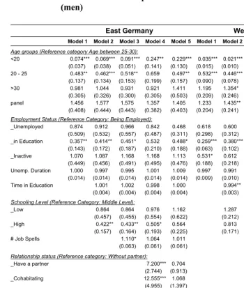
Table 7 displays the results for men, and follows the same approach as the one used in Table 6 (stepwise addition of controls). For men, we expected unemployment to have a negative effect on fertility timing, as stated in our first hypothesis. We failed to confirm this hypothesis, however. We found no significant association between unemployment and fertility timing in any of our models for men in East and West Germany. This is surprising because the theoretical prediction for men was less ambiguous than for women, since the theory for men predicts only an income effect from unemployment, but no substitution effect.
Regarding our unemployment duration variable, we faced the same difficulty for men as we did for women: the sample size was small. Particularly in East Germany, we had such a small number of transitions (90 events) that it is difficult to find significant effects when we test for short- versus long-run differences of unemployment duration. When we include unemployment duration linearly, it shows no significant effect on fertility timing. Thus, we cannot fully confirm Hypothesis 2b, which asserts that the impact of unemployment depends on its duration. This is in line with our expectations, but we need a more refined test for Hypothesis 2b.16
Our models for men indeed show the expected signs for the education variables, as did our model for women. Additionally, for West German men, we find that time spent in school has a negative effect, which is robust across all specifications. We also find a striking difference between East and West German men regarding the impact of schooling. For East German men, as for East German women, having a higher level of education delayed the timing of fertility by about 50% relative to having a middle level of education; whereas for West German men, we did not observe significantly different effects between middle and high levels of schooling.
16 To that end, in the next section we report interaction effects between unemployment duration and other
Table 7: Piecewise constant exponential models for the timing of the first birth (men)
East Germany West Germany
Model 1 Model 2 Model 3 Model 4 Model 5 Model 1 Model 2 Model 3 Model 4 Model 5
Age groups (Reference category Age between 25-30):
<20 0.074*** 0.069*** 0.091*** 0.247** 0.229*** 0.035*** 0.021*** 0.022*** 0.098*** 0.096***
(0.037) (0.038) (0.051) (0.141) (0.130) (0.015) (0.010) (0.010) (0.047) (0.047)
20 - 25 0.483** 0.462*** 0.518** 0.659 0.497** 0.532*** 0.446*** 0.459*** 0.791 0.614**
(0.137) (0.134) (0.153) (0.199) (0.157) (0.090) (0.078) (0.081) (0.141) (0.118)
>30 0.981 1.044 0.931 0.921 1.411 1.195 1.354* 1.310 1.288 1.561**
(0.305) (0.326) (0.300) (0.305) (0.503) (0.209) (0.246) (0.243) (0.239) (0.309)
panel 1.456 1.577 1.575 1.357 1.405 1.233 1.435** 1.422** 1.191 1.248
(0.408) (0.444) (0.443) (0.382) (0.403) (0.204) (0.241) (0.239) (0.204) (0.222)
Employment Status (Reference Category: Being Employed):
_Unemployed 0.874 0.912 0.966 0.842 0.468 0.618 0.600 0.623 0.694 0.591
(0.509) (0.532) (0.557) (0.487) (0.311) (0.298) (0.312) (0.322) (0.360) (0.332)
_in Education 0.357** 0.414** 0.451* 0.532 0.488* 0.259*** 0.380*** 0.394*** 0.591* 0.560**
(0.143) (0.172) (0.187) (0.210) (0.188) (0.063) (0.102) (0.107) (0.160) (0.159)
_Inactive 1.070 1.087 1.168 1.168 1.113 0.531* 0.612 0.630 0.720 0.602
(0.449) (0.456) (0.491) (0.495) (0.476) (0.188) (0.218) (0.225) (0.255) (0.240)
Unemp. Duration 1.000 0.997 0.995 1.001 1.009 0.997 0.991 0.989 1.008 1.007
(0.014) (0.014) (0.014) (0.014) (0.014) (0.009) (0.010) (0.010) (0.011) (0.012)
Time in Education 1.001 1.002 0.998 1.000 0.994** 0.994** 0.992*** 0.994**
(0.004) (0.004) (0.004) (0.004) (0.003) (0.003) (0.003) (0.003)
Schooling Level (Reference Category: Middle Level):
_Low 0.864 0.864 0.976 1.162 1.287 1.279 1.324* 1.154
(0.457) (0.455) (0.554) (0.622) (0.212) (0.211) (0.219) (0.200)
_High 0.422** 0.433** 0.505* 0.564 0.813 0.825 1.130 1.140
(0.157) (0.164) (0.193) (0.225) (0.171) (0.174) (0.243) (0.257)
# Job Spells 1.110* 1.064 1.011 1.033 0.935* 0.952
(0.063) (0.061) (0.061) (0.038) (0.036) (0.032)
Relationship status (Reference category: Without partner):
_Have a partner 7.200*** 0.704 6.823*** 3.286*
(2.744) (0.913) (2.197) (2.249)
_Cohabitating 12.555*** 1.068 16.861*** 8.461***
(4.955) (1.397) (5.481) (5.794)
_Marriage 29.567*** 3.780 68.640*** 36.655***
(12.702) (4.919) (21.646) (24.746)
Age of Partner 1.435*** 1.163***
(0.160) (0.061)
Age-Squared of Partner 0.991*** 0.996***
(0.002) (0.001)
Partner Human Capital 0.788** 0.890**
(0.082) (0.043)
Log likelihood -114.421 -110.347 -108.838 -64.749 -48.411 -243.179 -226.674 -226.309 -51.203 -41.325
Chi-Squared 183.815*** 191.492*** 194.508***282.686***303.499***550.268***559.836***560.565***910.778*** 882.875***
Number of Events 90 90 90 90 88 223 223 223 223 208
N 3471 3466 3466 3466 3257 8641 8466 8466 8466 8221
Interestingly, we find that partner characteristics have a stronger effect for men than for women. As the female partner’s human capital increases, fatherhood transitions are less likely by about 20% in East Germany, and by 10% in West Germany. This finding partially confirms Hypothesis 5a, which predicted a negative impact of the partner’s human capital on fatherhood decisions, especially for those with lower levels of education. (We provide further evidence concerning the less-educated subgroup in the next section.) It may be recalled that we found the husband’s human capital to have no effect on women’s motherhood transitions (see Table 6). This gender contrast is interesting because it suggests that the wife’s education (and perhaps her career) is more important for the timing of childbirth decisions, although testing this argument formally is beyond the scope of this paper.
4.3 Interaction effects
Some of our hypotheses suggest that the income effect or the substitution effect might be differentially stronger for women and men, depending on their educational attainment. If this is true, simply conditioning on education might not capture such differences in parenthood processes. For example, unemployment for highly educated individuals might imply a bigger income effect (loss) than for persons without much schooling. If the spouse is also highly educated, the importance of unemployment might also be very different, depending on the gender. Our Hypotheses 3 and 4 are formulated to test these variations in the impact of unemployment. To this end, we report a number of interaction effects for women and men, respectively, in Tables 8 and 9.
Table 8: Interaction effects on the timing of the first birth for women in East and West Germany
E ast G er m an y W est Ger m an y Mo d e l 1 M odel 2 M odel 3 Mo d e l 4 M odel 5 M odel 1 Mo d e l 2 Mo d e l 3 M odel 4 M odel 5
Level of Sc
ho ol ing (R ef er ence C at ego ry: M edi um ) _Low 1.753 2. 443* * 2. 463* * 2. 443* * 2. 463* * 1. 74 2* ** 1.562* ** 1. 562* ** 1 .5 4 6 *** 1.546* ** (0.825 ) (0 .9 8 2) (0 .9 9 0) (0 .9 8 2) (0 .9 9 0) (0 .2 52 ) (0.225 ) (0 .2 2 5) (0 .2 2 4) (0. 224 ) _Hi gh 0.349* ** 0. 529* 0. 524* 0. 529* 0. 524* 0. 61 8* ** 0.619* * 0. 620* * 0. 619* * 0.620* * (0.124 ) (0 .1 7 5) (0 .1 7 4) (0 .1 7 5) (0 .1 7 4) (0 .1 13 ) (0.119 ) (0 .1 1 9) (0 .1 1 9) (0. 120 ) E m pl o ym ent S tat us (Ref er ence Cat egor y: E m pl oyed) _Educat io n 0. 163* ** 0. 171* ** 0 .1 7 6 *** 0. 171* ** 0. 176* ** 0.218* ** 0.181* ** 0. 181* ** 0 .1 8 3 *** 0.184* ** (0 .0 5 0) (0 .0 5 4) (0 .0 5 5) (0 .0 5 4) (0 .0 5 5) (0.067 ) (0.058 ) (0 .0 5 8) (0 .0 5 9) (0. 059 ) _Unem pl oyed 1. 781* 1. 568 3. 052 1. 568 3. 057 0.876 0.921 0. 443 0. 920 0.449 (0 .5 7 7) (0 .5 5 1) (2 .2 2 0) (0 .5 5 1) (2 .2 2 8) (0.419 ) (0.426 ) (0 .4 8 8) (0 .4 2 6) (0. 495 ) _Inact ive 1. 612 1. 687 1. 706 1. 648 1. 798 1.494 1.697* 1. 701* 2. 528* 2.510* (0 .6 7 6) (0 .7 4 8) (0 .7 5 7) (2 .2 2 2) (2 .4 3 3) (0.421 ) (0.480 ) (0 .4 8 1) (1 .3 9 6) (1. 386 ) Unem p. Durati on 1. 011 1. 016* 1. 012 1. 016* 1. 012 1.006 0.989 0. 989 0. 989 0.989 (0 .0 1 0) (0 .0 0 9) (0 .0 0 9) (0 .0 0 9) (0 .0 0 9) (0.017 ) (0.012 ) (0 .0 1 2) (0 .0 1 2) (0. 012 ) _Low x (Une m p . Durati on) 1. 081 0.957* (0 .0 5 5) (0.023 ) _Hi gh x ( U nem p. D u ra tion) 1. 103* 0.988 (0 .0 5 6) (0.026 ) P a rtner' s E ducat ion 0. 876 0. 890 0. 875 0.891 0.969 0. 966 0. 973 0.970 (0 .0 7 3) (0 .0 7 5) (0 .0 7 4) (0.077 ) (0.037 ) (0 .0 3 7) (0 .0 3 8) (0. 038 ) (_U nem pl oyed) x (Partne r's Educ at io n) 0.844 1. 192 1.187 (0.143 ) (0.143 ) (0 .2 6 7) (0. 266 ) (_ In a ct ive ) x (Partner 's Educat io n) 0.988 0. 895 0.897 (0 .309 ) (0.304 ) (0 .1 2 5) (0. 125 ) Log-like lihood -50.057 -50. 968 -50.474 -50. 968 -50. 474 20.267 26. 904 27. 216 27.220 27.518 Chi -s quare d 424.74* ** 390. 62* ** 391.61* ** 390. 62* ** 391. 61 ** * 1142.17* ** 1 116. 48* ** 1117. 1* ** 1117.11* ** 1117.70* ** N 2807 2645 2645 2 645 2645 6596 6282 6282 6282 6282 Not e : On e ast e ri sk in di cates a si gn ifi cance le ve l oft 90% , t w o ast e ri sks in di ca te a le ve
l of 95%
, an d th re e ast e ri sk s in di ca te a le ve
l of 99%
. In the spec ifi ca tions 1, w e cont rol f or b ei ng in the p ane l s ur vey, tim e spent in educ at ion, r el ati ons hi p st atus. I n M o de ls 2 t
o 5 w
Table 8 reports the results of seven models with different sets of interactions for
women, which were run for East and West Germany separately.Model 1 includes only
the interaction term between education level and unemployment duration to capture the
potentially different meanings of this variable. Unemployment duration has a similar
impact on motherhood transitions for women with both low and high levels of education, relative to the middle-level group in East and West Germany.17 Strikingly, the impact is positive in East Germany and negative in West Germany. Specifically, we find that, in East Germany, an extra month of unemployment duration accelerates the
risk of transitioning to motherhood by about 11.5%18 for women in the highest
education category. For West German women in the lowest education category, an extra month of unemployment results in a small (approximately 4%) decline in risk.
Thus it appears that, in East Germany, highly educated women regard unemployment as an opportunity to have a child, especially as its duration increases. This result is somewhat surprising, but it is consistent with our finding in Section 4.1 that unemployment contributes to the risk of transitioning to motherhood only in East Germany. This also implies that, in East Germany, unemployment duration only delays fertility for women with middle levels of education. With these results, our Hypothesis 3 is partially confirmed. We find the precisely expected result for highly educated women in East Germany. However, our results do not confirm our expectations for women with low levels of education in general. On the contrary: we find a small negative impact of unemployment duration for these women in West Germany. Sample differences complicate a comparison of impact sizes between East and West Germany. Still, the effects are only marginally significant in both East and West Germany.
We now turn our attention to men, and consider the same interactions in Model 1 in Table 9. We find no statistically significant differences across education categories in the effect of unemployment duration on fatherhood transitions. If we assume for the moment that the absence of significant differences is due to a lack of analytical power (i.e., the small number of events), and not to the absence of a relationship between the variables, we can see that the coefficients are in the expected direction: we find that an additional month of unemployment has a positive effect for highly educated men, and no effect or a negative effect for less-educated men, reflecting the resources available.
17 Although the coefficients are similar in size (and in their standard deviation), it is obvious that we lack
statistical power. Thus, we only interpret the significant education categories.
18 This number is calculated using both coefficients of interaction components with the following formula:
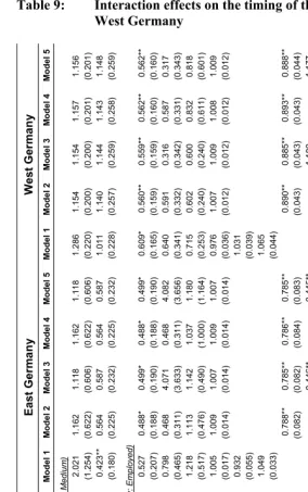
Table 9: Interaction effects on the timing of the first birth for men in East and West Germany East Ger m a n y Wes t G er m an y Mode l 1 Model 2 Model 3 Model 4 Model 5 Mode l 1 Mode l 2 M ode l 3 M ode l 4 M ode l 5 Lev el of S ch ool in g ( R ef er en ce Ca te gor y: M ed ium ) _L ow 2. 02 1 1. 16 2 1. 11 8 1. 16 2 1. 118 1. 28 6 1. 154 1. 15 4 1. 157 1. 15 6 (1 .2 54 ) (0. 622 ) (0 .6 06 ) (0 .6 22 ) (0 .6 06) (0. 220 ) (0 .2 00) (0 .2 00 ) (0. 20 1) (0 .2 01) _H ig h 0. 42 3** 0. 56 4 0. 58 7 0. 56 4 0. 587 1. 01 1 1. 140 1. 14 4 1. 143 1. 14 8 (0 .1 80 ) (0. 225 ) (0 .2 32 ) (0 .2 25 ) (0 .2 32) (0. 228 ) (0 .2 57) (0 .2 59 ) (0. 25 8) (0 .2 59) E m pl oym en t S ta tus ( R ef er enc e C at eg or y: E m pl oy ed) _ E duc at io n 0. 52 7 0. 48 8* 0. 49 9* 0. 48 8* 0. 499* 0. 60 9* 0. 560** 0. 55 9** 0. 562** 0. 56 2* * (0 .2 07 ) (0. 188 ) (0 .1 90 ) (0 .1 88 ) (0 .1 90) (0. 165 ) (0 .1 59) (0 .1 59 ) (0. 16 0) (0 .1 60) _U nem plo ye d 0. 79 8 0. 46 8 4. 07 1 0. 46 8 4. 082 0. 64 0 0. 591 0. 31 6 0. 587 0. 31 7 (0 .4 65 ) (0. 311 ) (3 .6 33 ) (0 .3 11 ) (3 .6 56) (0. 341 ) (0 .3 32) (0 .3 42 ) (0. 33 1) (0 .3 43) _I na ct ive 1. 21 8 1. 11 3 1. 14 2 1. 03 7 1. 180 0. 71 5 0. 602 0. 60 0 0. 832 0. 81 8 (0 .5 17 ) (0. 476 ) (0 .4 90 ) (1 .0 00 ) (1 .1 64) (0. 253 ) (0 .2 40) (0 .2 40 ) (0. 61 1) (0 .6 01) Un emp . D ura tion 1. 00 5 1. 00 9 1. 00 7 1. 00 9 1. 007 0. 97 6 1. 007 1. 00 9 1. 008 1. 00 9 (0 .0 17 ) (0. 014 ) (0 .0 14 ) (0 .0 14 ) (0 .0 14) (0. 036 ) (0 .0 12) (0 .0 12 ) (0. 01 2) (0 .0 12) _L ow x ( U ne m p. Du ra tio n ) 0. 93 2 1. 03 1 (0 .0 55 ) (0. 039 ) _H ig h x ( U nemp .D ur at ion ) 1. 04 9 1. 06 5 (0 .0 33 ) (0. 044 ) P ar tne r's Ed uc at io n 0. 78 8** 0. 78 5** 0. 78 6** 0. 785** 0. 890** 0. 88 5** 0. 893** 0. 88 8* * (0. 082 ) (0 .0 82 ) (0 .0 84 ) (0 .0 83) (0 .0 43) (0 .0 43 ) (0. 04 3) (0 .0 44) (_U ne m pl oy ed) x ( P ar tn er 's E du cat io n) 0. 44 6** 0. 445** 1. 18 0 1. 17 7 (0 .1 57 ) (0 .1 57) (0 .2 63 ) (0 .2 62) (_I na ct iv e) x ( P ar tner 's E duc at ion) 1. 01 9 0. 991 0. 915 0. 91 8 (0 .2 38 ) (0 .2 37) (0. 16 3) (0 .1 64) Lo g-like lih oo d -6 1. 94 0 -4 8. 41 1 -4 5. 441 -4 8. 408 -4 5. 44 1 -49. 71 8 -4 1. 325 -4 1. 04 4 -4 1. 20 2 -4 0. 93 1 C hi -s qua re d 28 8.31 *** 30 3. 50 *** 30 9. 44 *** 303. 51*** 30 9. 44 *** 913 .75* ** 88 2. 88* ** 883. 44*** 883 .1 3** * 88 3.67 *** N 3 466 32 57 32 57 32 57 32 57 84 66 82 21 82 21 82 21 8 221 N o te: O ne as ter isk indi ca te s a s ig ni fic an ce le vel o f 9 0% , t w o as ter is ks in di cat e a l ev el o f 95 %, an d th re e as ter is ks in di ca
te a l
Finally, Hypotheses 4a and 4b are concerned with the interaction between the partner’s human capital and unemployment. Hypothesis 4a suggests that unemployed men with highly educated partners will delay fatherhood. Models 2 to 5, shown in Table 9, consider different combinations of partner characteristics for men in East and West Germany. Overall, the partner’s education decreased the men’s likelihood of becoming a father by 10% to 20% in East and West Germany. Further, we find that each additional year of a partner’s education decreases the likelihood of fatherhood transitions for unemployed men by about 65% in East Germany. While partner education delays fatherhood in West Germany as well, its interaction with unemployment is not significant. This means that, in West Germany, additional education of the partner has a general negative effect for all men, but this effect does not vary by men’s employment status.
Moreover, the effect we observe for unemployment does not apply to men who are inactive: this interaction has no effect for men in both East and West Germany. Thus, Hypothesis 5a is confirmed in East Germany, but not in West Germany. It is unclear what exactly the absence of such an effect in West Germany means. First, we do not have information on the partner’s employment status. The partner’s education might be capturing part of the effect of the partner’s employment. If this is true, one interpretation might be that, when men are unemployed, the cost of an educated woman’s work interruptions due to childbirth might be bigger in East Germany than in West Germany, because East German wives are more likely to be employed than West German wives.
If we again consider Table 8 and apply the same hypothesis (5b) to women, we find that the husband’s education has no impact on women’s fertility timing across the board, and we cannot confirm that the husband’s education matters for childbirth decisions when a wife is either unemployed or inactive. Thus, based on the results of Models 2 to 5, we cannot confirm Hypothesis 5a.
4.4 Additional specifications and sensitivity analysis
4.4.1 Period-specific effects
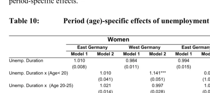
Hypothesis 2c is the only hypothesis that remains to be assessed. It suggests that the effect of unemployment varies in different stages of the life course. In order to capture life-course trends,19 we include period-specific effects of unemployment duration in
Table 10.20 We report two models for each country and for each sex. In the first model, we show the baseline model of overall unemployment duration (only the main effect). In the second model, we show the interaction between unemployment months by each sub-period of the baseline hazard (i.e., age group) on fertility timing. In both models, we again use Model 4 from Tables 6 and 7 as the baseline, to which we add a full set of period-specific effects.
Table 10: Period (age)-specific effects of unemployment spells
Women Men
East Germany West Germany East Germany West Germany Model 1 Model 2 Model 1 Model 2 Model 1 Model 2 Model 1 Model 2
Unemp. Duration 1.010 0.984 0.994 1.003
(0.008) (0.011) (0.015) (0.011)
Unemp. Duration x (Age< 20) 1.010 1.141*** 0.001 1.011
(0.041) (0.051) (1.034) (0.076)
Unemp. Duration x (Age 20-25) 1.021 0.997 1.008 1.013
(0.014) (0.028) (0.027) (0.015)
Unemp. Duration x (Age 25-30) 0.995 0.979 0.980 0.967
(0.020) (0.017) (0.027) (0.025)
Unemp. Duration x (Age > 30) 1.016 0.983 0.995 1.011
(0.010) (0.016) (0.017) (0.012)
# of Events 139 139 289 289 87 87 208 208
Log-likelihood -81.286 -85.965 -19.675 -18.635 -67.739 -70.894 -81.192 -81.755
Chi-squared 4318.571*** 4356.662*** 7508.538*** 7515.606*** 2853.629*** 2897.187*** 6402.993*** 6414.605***
N 2760 2760 6523 6523 3445 3445 8414 8414
Note: One asterisk indicates a significance level of 90%, two asterisks indicate a level of 95%, and three asterisks indicate a level of 99%. In all the specifications, we control for being in the panel survey, time spent in education, and all the previous covariates related to employment status and relationship status. Coefficients indicate hazard ratios and standard errors are in parentheses.
Model 2 in Table 10 shows the trends of unemployment duration over the life course on fertility timing. Hypothesis 2c predicted an initial strong negative effect of unemployment duration for younger women that fades away with age. Our models reject this hypothesis. For East German women21 and for men in the East and West, we find that the effect of unemployment duration does not significantly differ across age groups. It is also important to keep in mind that “the early stages” mentioned in the theoretical arguments about the impact of unemployment duration often refer to the early stages of work life. However, because the fertility window starts at the age of 16
20 We also examined, but do not report, period-specific effects of job changes. The results are available upon
request.
21 The first period (age< 20) is pre-1991, when unemployment had not yet started, as indicated by the zero
in our data, our “early” age group (age<20) usually coincides with time enrolled in school. In this context, the significant coefficient for the first age group in West Germany is likely driven by a very select, small group of women in the labor market, and therefore should not be interpreted substantially.
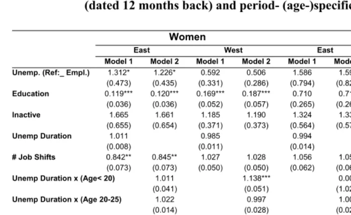
4.4.2 Sensitivity check for timing of conception
While some studies directly model the timing of the first birth, most researchers subtract nine months (or a year) from the date of birth to counter the obvious endogeneity problem, just as we did in this paper. However, as mentioned previously, it could be argued that the timing of conception decisions may differ from the timing of conception itself. The extant literature using event history models often ignores this difference. The difficulty is that the distribution of time that has elapsed between the decision and the actual conception is unknown. To find out whether our estimations are sensitive to this time difference, we tested our models by subtracting 8, 10, 11 and 12 months from the date of the first birth.
In Table 11, we show only the specification in which we subtract 12 months from the date of birth, instead of nine months. Model 1 simply replicates the baseline model (i.e., Model 4 in Tables 6 and 7) with this new dependent variable. Due to space limitations, control variables are not shown in this table. Three coefficients for the main explanatory variables related to unemployment are reported. Model 2 reports the period-specific effects of unemployment duration.