Numerical Solution of

(1)

Numerical Solution of

Partial Differential Equations

by

Gordon C. Everstine

(2)

(3)

Preface

These lecture notes are intended to supplement a one-semester graduate-level engineering course at The George Washington University in numerical methods for the solution of par-tial differenpar-tial equations. Both finite difference and finite element methods are included. The main prerequisite is a standard undergraduate calculus sequence including ordinary differential equations. In general, the mix of topics and level of presentation are aimed at upper-level undergraduates and first-year graduate students in mechanical, aerospace, and civil engineering.

Gordon Everstine

(4)

(5)

List of Figures

1 1-DOF Mass-Spring System. . . 1

2 Simply-Supported Beam With Distributed Load. . . 2

3 Finite Difference Approximations to Derivatives. . . 6

4 The Shooting Method. . . 11

(7)

6 Heat Equation Stencil for Explicit Finite Difference Algorithm. . . 17

7 Heat Equation Stencil forr = 1/10. . . 17

8 Heat Equation Stencils forr = 1/2 and r= 1. . . 17

9 Explicit Finite Difference Solution With r= 0.48. . . 18

10 Explicit Finite Difference Solution With r= 0.52. . . 19

11 Mesh for Crank-Nicolson. . . 20

12 Stencil for Crank-Nicolson Algorithm. . . 20

13 Treatment of Derivative Boundary Conditions. . . 21

14 Propagation of Initial Displacement. . . 23

15 Initial Velocity Function. . . 24

16 Propagation of Initial Velocity. . . 24

17 Domains of Influence and Dependence. . . 25

18 Mesh for Explicit Solution of Wave Equation. . . 26

19 Stencil for Explicit Solution of Wave Equation. . . 26

20 Domains of Dependence forr >1. . . 27

21 Finite Difference Mesh at Nonreflecting Boundary. . . 28

22 Finite Length Simulation of an Infinite Bar. . . 30

23 Laplace’s Equation on Rectangular Domain. . . 31

24 Finite Difference Grid on Rectangular Domain. . . 31

25 The Neighborhood of Point (i, j). . . 32

26 20-Point Finite Difference Mesh. . . 32

27 Laplace’s Equation With Dirichlet and Neumann B.C. . . 33

28 Treatment of Neumann Boundary Conditions. . . 34

29 2-DOF Mass-Spring System. . . 34

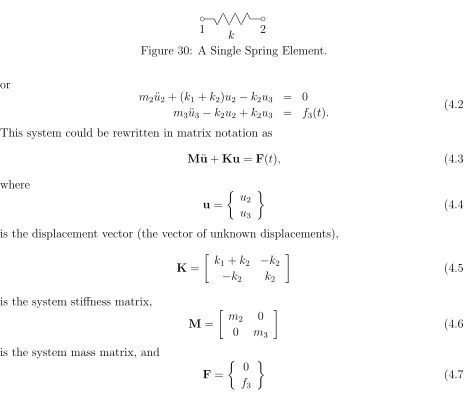
30 A Single Spring Element. . . 35

31 3-DOF Spring System. . . 36

32 Spring System With Constraint. . . 37

33 4-DOF Spring System. . . 37

34 Pin-Jointed Rod Element. . . 39

35 Truss Structure Modeled With Pin-Jointed Rods. . . 39

36 The Degrees of Freedom for a Pin-Jointed Rod Element in 2-D. . . 40

37 Computing 2-D Stiffness of Pin-Jointed Rod. . . 40

38 Pin-Jointed Frame Example. . . 41

39 Example With Reactions and Loads at Same DOF. . . 42

40 Large Spring Approach to Constraints. . . 43

41 DOF for Beam in Flexure (2-D). . . 44

42 The Beam Problem Associated With Column 1. . . 44

43 The Beam Problem Associated With Column 2. . . 45

44 DOF for 2-D Beam Element. . . 45

45 Plate With Constraints and Loads. . . 46

46 DOF for the Linear Triangular Membrane Element. . . 46

47 Element Coordinate Systems in the Finite Element Method. . . 50

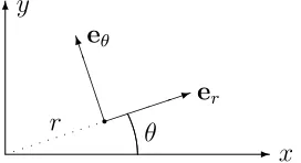
48 Basis Vectors in Polar Coordinate System. . . 50

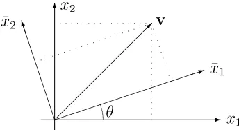
49 Change of Basis. . . 51

(8)

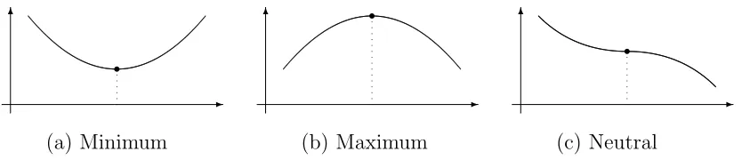
51 Minimum, Maximum, and Neutral Stationary Values. . . 58

52 Curve of Minimum Length Between Two Points. . . 60

53 The Brachistochrone Problem. . . 61

54 Several Brachistochrone Solutions. . . 63

55 A Constrained Minimization Problem. . . 64

56 Two-Dimensional Finite Element Mesh. . . 70

57 Triangular Finite Element. . . 70

58 Axial Member (Pin-Jointed Truss Element). . . 72

59 Neumannn Boundary Condition at Internal Boundary. . . 74

60 Two Adjacent Finite Elements. . . 75

61 Triangular Mesh at Boundary. . . 78

62 Discontinuous Function. . . 81

63 Compatibility at an Element Boundary. . . 82

64 A Vector Analogy for Galerkin’s Method. . . 83

65 Potential Flow Around Solid Body. . . 86

66 Streamlines Around Circular Cylinder. . . 87

67 Symmetry With Respect to y= 0. . . 87

68 Antisymmetry With Respect to x= 0. . . 88

69 Boundary Value Problem for Flow Around Circular Cylinder. . . 88

70 The Free Surface Problem. . . 89

71 The Complex Amplitude. . . 90

72 Phasor Addition. . . 91

73 2-D Wave Maker: Time Domain. . . 91

74 Graphical Solution of ω2_/α₌_g_{tanh(αd). . . .} ₉₃

75 2-D Wave Maker: Frequency Domain. . . 93

(9)

1 Numerical Solution of Ordinary Differential

Equa-tions

An ordinary differential equation (ODE) is an equation that involves an unknown function (the dependent variable) and some of its derivatives with respect to a single independent variable. Annth-order equation has the highest order derivative of order n:

f x, y, y0, y00, . . . , y(n)= 0 for a≤x≤b, (1.1) where y = y(x), and y(n) _{denotes the} _{nth derivative with respect to}_{x. An} _{nth-order ODE}

requires the specification ofnconditions to assure uniqueness of the solution. If all conditions are imposed at x = a, the conditions are called initial conditions (I.C.), and the problem is an initial value problem (IVP). If the conditions are imposed at both x = a and x = b, the conditions are called boundary conditions (B.C.), and the problem is a boundary value problem (BVP).

For example, consider the initial value problem

mu¨+ku=f(t)

u(0) = 5, u(0) = 0,˙ (1.2)

where u = u(t), and dots denote differentiation with respect to the time t. This equation describes a one-degree-of-freedom mass-spring system which is released from rest and sub-jected to a time-dependent force, as illustrated in Fig. 1. Initial value problems generally arise in time-dependent situations.

An example of a boundary value problem is shown in Fig. 2, for which the differential equation is

 



EIu00(x) =M(x) = F L

2 x−F x x

2

u(0) =u(L) = 0,

(1.3)

where the independent variable x is the distance from the left end, u is the transverse displacement, and M(x) is the internal bending moment at x. Boundary value problems generally arise in static (time-independent) situations. As we will see, IVPs and BVPs must be treated differently numerically.

A system of n first-order ODEs has the form 

   

   

y₁0(x) = f1(x, y1, y2, . . . , yn)

y₂0(x) = f2(x, y1, y2, . . . , yn)

.. .

y_n0(x) = fn(x, y1, y2, . . . , yn)

(1.4)

AAAA

k

m

- u(t)

e e

- f(t)

(10)

? ? ? ? ? ? ? ? ? ? ?

@ @

F (N/m)

L

-Figure 2: Simply-Supported Beam With Distributed Load.

fora≤x≤b. A singlenth-order ODE is equivalent to a system ofn first-order ODEs. This equivalence can be seen by defining a new set of unknowns y1, y2, . . . , yn such that y1 =y,

y2 =y0,y3 =y00,. . . ,yn=y(n−1). For example, consider the third-order IVP

y000 =xy0+ex_y₊_x2_{+ 1, x}_≥₀

y(0) = 1, y0(0) = 0, y00(0) = −1. (1.5)

To obtain an equivalent first-order system, define y1 =y,y2 =y0, y3 =y00 to obtain

 



y₁0 =y2

y₂0 =y3

y₃0 =xy2+exy1+x2+ 1

(1.6)

with initial conditions y1(0) = 1, y2(0) = 0,y3(0) =−1.

1.1 Euler’s Method

This method is the simplest of the numerical methods for solving initial value problems. Consider the IVP

y0(x) = f(x, y), x≥a

y(a) = η. (1.7)

To effect a numerical solution, we discretize the x-axis:

a=x0 < x1 < x2 <· · ·,

where, for uniform spacing,

xi−xi−1 =h, (1.8)

and his considered small. With this discretization, we can approximate the derivative y0(x) with the forward finite difference

y0(x)≈ y(x+h)−y(x)

h . (1.9)

If we let yk represent the numerical approximation to y(xk), then

y0(xk)≈

yk+1−yk

(11)

Thus, a numerical (difference) approximation to the ODE, Eq. 1.7, is yk+1−yk

h =f(xk, yk), k= 0,1,2, . . . (1.11) or

yk+1 =yk+hf(xk, yk), k= 0,1,2, . . .

y0 =η.

(1.12)

This recursive algorithm is called Euler’s method.

1.2 Truncation Error for Euler’s Method

There are two types of error that arise in numerical methods: truncation error (which arises primarily from a discretization process) and rounding error (which arises from the finiteness of number representations in the computer). Refining a mesh to reduce the truncation error often causes the rounding error to increase.

To estimate the truncation error for Euler’s method, we first recall Taylor’s theorem with remainder, which states that a function f(x) can be expanded in a series about the point x=c:

f(x) = f(c) +f0(c)(x−c) +f 00_(c)

2! (x−c)

2₊_{· · ·}₊f(n)(c)

n! (x−c)

n₊f(n+1)(ξ)

(n+ 1)! (x−c)

n+1_, _(1.13)

where ξ is betweenx and c. The last term in Eq. 1.13 is referred to as the remainder term. Note also that Eq. 1.13 is an equality, not an approximation.

In Eq. 1.13, let x=xk+1 and c=xk, in which case

y(xk+1) = y(xk) +hy0(xk) +

1 2h

2_y00

(ξk), (1.14)

where xk≤ξk ≤xk+1.

Since y satisfies the ODE, Eq. 1.7,

y0(xk) = f(xk, y(xk)), (1.15)

where y(xk) is the actual solution at xk. Hence,

y(xk+1) =y(xk) +hf(xk, y(xk)) +

1 2h

2

y00(ξk). (1.16)

Like Eq. 1.13, this equation is an equality, not an approximation.

By comparing this last equation to Euler’s approximation, Eq. 1.12, it is clear that Euler’s method is obtained by omitting the remainder term 1₂h2y00(ξk) in the Taylor expansion of

y(xk+1) at the point xk. The omitted term accounts for the truncation error in Euler’s

methodat each step. This error is a local error, since the error occurs at each step regardless of the error in the previous step. The accumulation of local errors is referred to as theglobal error, which is the more important error but much more difficult to compute.

(12)

1.3 Runge-Kutta Methods

Euler’s method is a first-order method, since it was obtained by omitting terms in the Taylor series expansion containing powers of hgreater than one. To derive a second-order method, we again use Taylor’s theorem with remainder to obtain

y(xk+1) = y(xk) +hy0(xk) +

1 2h

2_y00 (xk) +

1 6h

3_y000

(ξk) (1.17)

for some ξk such that xk≤ξk ≤xk+1. Since, from the ODE (Eq. 1.7),

y0(xk) = f(xk, y(xk)), (1.18)

we can approximate

y00(x) = df(x, y(x))

dx =

f(x+h, y(x+h))−f(x, y(x))

h +O(h) (1.19)

where we use the “big O” notation O(h) to represent terms of order h as h → 0. [For example, 2h3 =O(h3), 3h2+ 5h4 =O(h2),h2O(h) =O(h3), and −287h4e−h =O(h4).] From these last two equations, Eq. 1.17 can then be written as

y(xk+1) = y(xk) +hf(xk, y(xk)) +

h

2[f(xk+1, y(xk+1))−f(xk, y(xk))] +O(h

3_), _(1.20)

which leads (after combining terms) to the difference equation

yk+1 =yk+

1

2h[f(xk, yk) +f(xk+1, yk+1)]. (1.21) This formula is a second-order approximation to the original differential equation y0(x) = f(x, y) (Eq. 1.7), but it is an inconvenient approximation, since yk+1 appears on both sides

of the formula. (Such a formula is called animplicit method, sinceyk+1 is defined implicitly.

An explicit method would haveyk+1 appear only on the left-hand side.)

To obtain instead an explicit formula, we use the approximation

yk+1 =yk+hf(xk, yk) (1.22)

to obtain

yk+1 =yk+

1

2h[f(xk, yk) +f(xk+1, yk+hf(xk, yk))]. (1.23) This formula is the Runge-Kutta formula of second order. Other higher-order formulas can be derived similarly. For example, a fourth-order formula turns out to be popular in applications.

We illustrate the implementation of the second-order Runge-Kutta formula, Eq. 1.23, with the following algorithm. We first make the following three definitions:

ak=f(xk, yk), (1.24)

(13)

ck =f(xk+1, bk), (1.26)

in which case

yk+1 =yk+

1

2h(ak+ck). (1.27)

The calculations can then be performed conveniently with the following spreadsheet:

k xk yk ak bk ck yk+1

0 1 2 .. .

1.4 Systems of Equations

The methods just derived can be extended directly to systems of equations. Consider the initial value problem involving two equations:

 



y0(x) =f(x, y(x), z(x)) z0(x) =g(x, y(x), z(x)) y(a) =η, z(a) = ξ.

(1.28)

We recall from Eq. 1.12 that, for one equation, Euler’s method uses the recursive formula

yk+1 =yk+hf(xk, yk). (1.29)

This formula is directly extendible to two equations as 





yk+1 =yk+hf(xk, yk, zk)

zk+1 =zk+hg(xk, yk, zk)

y0 =η, z0 =ξ.

(1.30)

We recall from Eq. 1.23 that, for one equation, the second-order Runge-Kutta method uses the recursive formula

yk+1 =yk+

1

2h[f(xk, yk) +f(xk+1, yk+hf(xk, yk))]. (1.31) For two equations, this formula becomes

  

 

yk+1 =yk+ 1₂h[f(xk, yk, zk) +f(xk+1, yk+hf(xk, yk, zk), zk+hg(xk, yk, zk))]

zk+1 =zk+ 1₂h[g(xk, yk, zk) +g(xk+1, yk+hf(xk, yk, zk), zk+hg(xk, yk, zk))]

y0 =η, z0 =ξ.

(14)

-6

x y(x)

x−h x x+h

s

H H

Y backward

difference

H H

Y forward

difference

H H j

central difference

Figure 3: Finite Difference Approximations to Derivatives.

1.5 Finite Differences

Before addressing boundary value problems, we want to develop further the notion of finite difference approximation of derivatives.

Consider a functiony(x) for which we want to compute the derivativey0(x) at some point x. If we discretize the x-axis with uniform spacing h, we could approximate the derivative using the forward difference formula

y0(x)≈ y(x+h)−y(x)

h , (1.33)

which is the slope of the line to the right of x (Fig. 3). We could also approximate the derivative using the backward difference formula

y0(x)≈ y(x)−y(x−h)

h , (1.34)

which is the slope of the line to the left of x. Since, in general, there is no basis for choosing one of these approximations over the other, an intuitively more appealing approximation results from the average of these formulas:

y0(x)≈ 1

2

y(x+h)−y(x)

h +

y(x)−y(x−h) h

(1.35)

or

y0(x)≈ y(x+h)−y(x−h)

2h . (1.36)

(15)

Similar approximations can be derived for second derivatives. Using forward differences,

y00(x)≈ y

0_(x₊_h)₋_y0_(x) h

≈ y(x+ 2h)−y(x+h)

h2 −

y(x+h)−y(x) h2

= y(x+ 2h)−2y(x+h) +y(x)

h2 . (1.37)

This formula, which involves three points forward ofx, is the forward difference approxima-tion to the second derivative. Similarly, using backward differences,

y00(x)≈ y

0_(x)₋_y0_(x₋_h) h

≈ y(x)−y(x−h)

h2 −

y(x−h)−y(x−2h) h2

= y(x)−2y(x−h) +y(x−2h)

h2 . (1.38)

This formula, which involves three points backward ofx, is the backward difference approx-imation to the second derivative. The central finite difference approxapprox-imation to the second derivative uses instead the three points which bracketx:

y00(x)≈ y(x+h)−2y(x) +y(x−h)

h2 . (1.39)

This last result can also be obtained by using forward differences for the second derivative followed by backward differences for the first derivatives, or vice versa.

The central difference formula for second derivatives can alternatively be derived using Taylor series expansions:

y(x+h) =y(x) +hy0(x) + h

2

2 y 00

(x) + h

3

6 y 000

(x) +O(h4). (1.40)

Similarly, by replacing h by−h,

y(x−h) = y(x)−hy0(x) + h

2

2 y 00

(x)−h 3

6y 000

(x) +O(h4). (1.41)

The addition of these two equations yields

y(x+h) +y(x−h) = 2y(x) +h2y00(x) +O(h4) (1.42)

or

y00(x) = y(x+h)−2y(x) +y(x−h)

h2 +O(h

2_), _(1.43)

(16)

1.6 Boundary Value Problems

The techniques for initial value problems (IVPs) are, in general, not directly applicable to boundary value problems (BVPs). Consider the BVP

y00(x) =f(x, y, y0), a≤x≤b y(a) = η1, y(b) =η2.

(1.44)

This equation could be nonlinear, depending on f. The methods used for IVPs started at one end (x =a) and computed the solution step by step for increasing x. For a BVP, not enough information is given at either endpoint to allow a step-by-step solution.

Consider first a special case of Eq. 1.44 for which the right-hand side depends only on x and y:

y00(x) = f(x, y), a≤x≤b y(a) =η1, y(b) = η2.

(1.45)

Subdivide the interval (a, b) into n equal subintervals:

h= b−a

n , (1.46)

in which case

xk =a+kh, k= 0,1,2, . . . , n. (1.47)

Let yk denote the numerical approximation to the exact solution at xk. That is,

yk≈y(xk). (1.48)

Then, if we use a central difference approximation to the second derivative in Eq. 1.45, the ODE can be approximated by

y(xk−1)−2y(xk) +y(xk+1)

h2 ≈f(xk, yk), (1.49)

which suggests the difference equation

yk−1−2yk+yk+1 =h2f(xk, yk), k= 1,2,3, . . . , n−1. (1.50)

Since this system of equations has n−1 equations in n+ 1 unknowns, the two boundary conditions are needed to obtain a nonsingular system:

y0 =η1, yn =η2. (1.51)

The resulting system is thus

−2y1 + y2 = −η1+h2f(x1, y1)

y1 − 2y2 + y3 = h2f(x2, y2)

y2 − 2y3 + y4 = h2f(x3, y3)

y3 − 2y4 + y5 = h2f(x4, y4)

.. .

yn−2 − 2yn−1 = −η2+h2f(xn−1, yn−1),

(1.52)

(17)

1.6.1 Example

Consider

y00=−y(x), 0≤x≤π/2

y(0) = 1, y(π/2) = 0. (1.53)

In Eq. 1.45, f(x, y) = −y, η1 = 1, η2 = 0. Thus, the right-hand side of the ith equation in

Eq. 1.52 has −h2_y

i, which can be moved to the left-hand side to yield the system

−(2−h2)y1 + y2 = −1

y1 − (2−h2)y2 + y3 = 0

y2 − (2−h2)y3 + y4 = 0

.. . yn−2 − (2−h2)yn−1 = 0.

(1.54)

We first solve this tridiagonal system of simultaneous equations withn = 8 (i.e., h=π/16), and compare with the exact solutiony(x) = cosx:

Exact Absolute %

k xk yk y(xk) Error Error

0 0 1 1 0 0

1 0.1963495 0.9812186 0.9807853 0.0004334 0.0441845 2 0.3926991 0.9246082 0.9238795 0.0007287 0.0788715 3 0.5890486 0.8323512 0.8314696 0.0008816 0.1060315 4 0.7853982 0.7080045 0.7071068 0.0008977 0.1269565 5 0.9817477 0.5563620 0.5555702 0.0007917 0.1425085 6 1.1780972 0.3832699 0.3826834 0.0005865 0.1532604 7 1.3744468 0.1954016 0.1950903 0.0003113 0.1595767

8 1.5707963 0 0 0 0

We then solve this system with n= 40 (h=π/80):

Exact Absolute %

k xk yk y(xk) Error Error

0 0 1 1 0 0

5 0.1963495 0.9808025 0.9807853 0.0000172 0.0017571 10 0.3926991 0.9239085 0.9238795 0.0000290 0.0031363 15 0.5890486 0.8315047 0.8314696 0.0000351 0.0042161 20 0.7853982 0.7071425 0.7071068 0.0000357 0.0050479 25 0.9817477 0.5556017 0.5555702 0.0000315 0.0056660 30 1.1780972 0.3827068 0.3826834 0.0000233 0.0060933 35 1.3744468 0.1951027 0.1950903 0.0000124 0.0063443

40 1.5707963 0 0 0 0

(18)

1.6.2 Solving Tridiagonal Systems

Tridiagonal systems are particularly easy (and fast) to solve using Gaussian elimination. It is convenient to solve such systems using the following notation:

d1x1 + u1x2 = b1

l2x1 + d2x2 + u2x3 = b2

l3x2 + d3x3 + u3x4 = b3

.. . lnxn−1 + dnxn = bn,

      

     

(1.55)

where di, ui, and li are, respectively, the diagonal, upper, and lower matrix entries in Row

i. All coefficients can now be stored in three one-dimensional arrays, D(·), U(·), and L(·), instead of a full two-dimensional array A(I,J). The solution algorithm (reduction to upper triangular form by Gaussian elimination followed by back-solving) can now be summarized as follows:

1. For k = 1,2, . . . , n−1: [k = pivot row]

(a) m=−lk+1/dk [m = multiplier needed to annihilate term below]

(b) dk+1 =dk+1+muk [new diagonal entry in next row]

(c) bk+1 =bk+1+mbk [new rhs in next row]

2. xn=bn/dn [start of back-solve]

3. For k =n−1, n−2, . . . ,1: [back-solve loop] (a) xk= (bk−ukxk+1)/dk

Tridiagonal systems arise in a variety of applications, including the Crank-Nicolson finite difference method for solving parabolic partial differential equations.

1.7 Shooting Methods

Shooting methods provide a way to convert a boundary value problem to a trial-and-error initial value problem. It is useful to have additional ways to solve BVPs, particularly if the equations are nonlinear.

Consider the following two-point BVP: 





y00 =f(x, y, y0), a≤x≤b y(a) = A

y(b) =B.

(1.56)

To solve this problem using the shooting method, we compute solutions of the IVP 





y00 =f(x, y, y0), x≥a y(a) =A

y0(a) = M

(19)

-6

x y

M1

M2

a _b

A

r

6

?

B

Figure 4: The Shooting Method.

for various values of M (the slope at the left end of the domain) until two solutions, one with y(b)< B and the other with y(b) > B, have been found (Fig. 4). The initial slope M can then be interpolated until a solution is found (i.e., y(b) =B).

2 Partial Differential Equations

A partial differential equation (PDE) is an equation that involves an unknown function (the dependent variable) and some of its partial derivatives with respect to two or more independent variables. An nth-order equation has the highest order derivative of order n.

2.1 Classical Equations of Mathematical Physics

1. Laplace’s equation (the potential equation)

∇2φ= 0 (2.1)

In Cartesian coordinates, the vector operator del is defined as

∇=ex

∂ ∂x +ey

∂ ∂y +ez

∂

∂z. (2.2)

∇2 _{is referred to as the Laplacian operator and given by}

∇2 ₌_{∇ · ∇}₌ ∂2

∂x2 +

∂2

∂y2 +

∂2

∂z2. (2.3)

Thus, Laplace’s equation in Cartesian coordinates is ∂2_φ

∂x2 +

∂2_φ

∂y2 +

∂2_φ

∂z2 = 0. (2.4)

In cylindrical coordinates, the Laplacian is

∇2_φ₌ 1

r ∂ ∂r

r∂φ

∂r

+ 1 r2

∂2φ ∂θ2 +

∂2φ

∂z2. (2.5)

(20)

heat conduction with no sources (in which case φ is the temperature), and torsion of bars in elasticity (in which case φ(x, y) is the warping function). Functions which satisfy Laplace’s equation are referred to as harmonic functions.

2. Poisson’s equation

∇2_φ₊_g _{= 0} _(2.6)

This equation arises in steady-state heat conduction with distributed sources (φ = temperature) and torsion of bars in elasticity (in which case φ(x, y) is the stress func-tion).

3. wave equation

∇2φ= 1

c2φ¨ (2.7)

In this equation, dots denote time derivatives, e.g.,

¨ φ= ∂

2_φ

∂t2, (2.8)

and c is the speed of propagation. The wave equation arises in several physical situa-tions:

(a) transverse vibrations of a string

For this one-dimensional problem, φ = φ(x, t) is the transverse displacement of the string, and

c= s

T

ρA, (2.9)

whereT is the string tension, ρ is the density of the string material, andAis the cross-sectional area of the string. The denominatorρA is mass per unit length. (b) longitudinal vibrations of a bar

For this one-dimensional problem, φ = φ(x, t) represents the longitudinal dis-placement, and

c= s

E

ρ, (2.10)

whereE and ρ are, respectively, the modulus of elasticity and density of the bar material.

(c) transverse vibrations of a membrane

For this two-dimensional problem,φ =φ(x, y, t) is the transverse displacement of the membrane (e.g., drum head), and

c= r

T

m, (2.11)

(21)

(d) acoustics

For this three-dimensional problem,φ=φ(x, y, z, t) is the fluid pressure or veloc-ity potential, andcis the speed of sound, where

c= s

B

ρ, (2.12)

whereB =ρc2 is the fluid bulk modulus, and ρ is the density. 4. Helmholtz equation (reduced wave equation)

∇2_φ₊_k2_φ_{= 0} _(2.13)

The Helmholtz equation is the time-harmonic form of the wave equation, in which inter-est is rinter-estricted to functions which vary sinusoidally in time. To obtain the Helmholtz equation, we substitute

φ(x, y, z, t) = φ0(x, y, z) cosωt (2.14)

into the wave equation, Eq. 2.7, to obtain

∇2_φ

0cosωt=−

ω2

c2φ0cosωt. (2.15)

If we define the wave number k =ω/c, this equation becomes

∇2φ0+k2φ0 = 0. (2.16)

With the understanding that the unknown depends only on the spacial variables, the subscript is unnecessary, and we obtain the Helmholtz equation, Eq. 2.13. This equa-tion arises in steady-state (time-harmonic) situaequa-tions involving the wave equaequa-tion, e.g., steady-state acoustics.

5. heat equation

∇ ·(k∇φ) +Q=ρcφ˙ (2.17) In this equation,φrepresents the temperatureT,k is the thermal conductivity,Qis the internal heat generation per unit volume per unit time,ρ is the material density, andc is the material specific heat (the heat required per unit mass to raise the temperature by one degree). The thermal conductivitykis defined by Fourier’s law of heat conduction:

ˆ

qx=−kA

dT

dx, (2.18)

where ˆqx is the rate of heat conduction (energy per unit time) with typical units J/s

or BTU/hr, and A is the area through which the heat flows. Alternatively, Fourier’s law is written

qx =−k

dT

dx, (2.19)

whereqx is energy per unit time per unit area (with typical units J/(s·m2). There are

(22)

(a) homogeneous material (k = constant):

k∇2φ+Q=ρcφ˙ (2.20)

(b) homogeneous material, steady-state (time-independent):

∇2_φ₌₋Q

k (Poisson’s equation) (2.21) (c) homogeneous material, steady-state, no sources (Q= 0):

∇2φ = 0 (Laplace’s equation) (2.22)

2.2 Classification of Partial Differential Equations

Of the classical PDEs summarized in the preceding section, some involve time, and some don’t, so presumably their solutions would exhibit fundamental differences. Of those that involve time (wave and heat equations), the order of the time derivative is different, so the fundamental character of their solutions may also differ. Both these speculations turn out to be true.

Consider the general, second-order, linear partial differential equation in two variables Auxx+Buxy +Cuyy+Dux+Euy+F u=G, (2.23)

where the coefficients are functions of the independent variables x and y (i.e., A=A(x, y), B =B(x, y), etc.), and we have used subscripts to denote partial derivatives, e.g.,

uxx =

∂2u

∂x2. (2.24)

The quantity B2₋_4AC _{is referred to as the} _discriminant _{of the equation. The behavior of}

the solution of Eq. 2.23 depends on the sign of the discriminant according to the following table:

B2 ₋_4AC _{Equation Type} _{Typical Physics Described}

<0 Elliptic Steady-state phenomena

= 0 Parabolic Heat flow and diffusion processes >0 Hyperbolic Vibrating systems and wave motion

The names elliptic, parabolic, and hyperbolic arise from the analogy with the conic sections in analytic geometry.

Given these definitions, we can classify the common equations of mathematical physics already encountered as follows:

Name Eq. Number Eq. in Two Variables A, B, C Type Laplace Eq. 2.1 uxx+uyy = 0 A=C = 1, B = 0 Elliptic

Poisson Eq. 2.6 uxx+uyy =−g A=C = 1, B = 0 Elliptic

Wave Eq. 2.7 uxx−uyy/c2 = 0 A= 1, C =−1/c2, B = 0 Hyperbolic

Helmholtz Eq. 2.13 uxx+uyy+k2u= 0 A=C = 1, B = 0 Elliptic

(23)

In the wave and heat equations in the above table, y represents the time variable. The behavior of the solutions of equations of different types differs. Elliptic equations characterize static (independent) situations, and the other two types of equations characterize time-dependent situations.

2.3 Transformation to Nondimensional Form

It is often convenient, when solving equations, to transform the equation to a nondimensional form. Consider, for example, the one-dimensional wave equation

∂2u ∂x2 =

1 c2

∂2u

∂t2, (2.25)

where u is displacement (of dimension length), t is time, and c is the speed of propagation (of dimension length/time). Let L represent some characteristic length associated with the problem. We define the nondimensional variables

¯ x= x

L, u¯= u

L, t¯= ct

L, (2.26)

in which case the derivatives in Eq. 2.25 become ∂u

∂x =

∂(L¯u) ∂(L¯x) =

∂u¯

∂x¯, (2.27)

∂2_u

∂x2 =

∂ ∂x ∂u ∂x = ∂ ∂x

∂u¯ ∂x¯

= ∂

∂x¯

∂u¯ ∂x¯

d¯x dx =

1 L

∂2_u_¯

∂x¯2, (2.28)

∂u ∂t =

∂(L¯u) ∂(L¯t/c) =c

∂u¯

∂t¯, (2.29)

∂2_u

∂t2 =

∂ ∂t ∂u ∂t = ∂ ∂t

c∂u¯ ∂¯t

=c ∂

∂¯t

∂u¯ ∂¯t

d¯t dt =c

∂2_u_¯

∂¯t2

c L =

c2

L ∂2_u_¯

∂t¯2. (2.30)

Thus, from Eq. 2.25,

1 L

∂2_u_¯

∂x¯2 =

1 c2 ·

c2

L ∂2_u_¯

∂¯t2 (2.31)

or

∂2_u_¯

∂x¯2 =

∂2_u_¯

∂¯t2. (2.32)

This is the nondimensional wave equation.

This last equation can also be obtained more easily by direct substitution of Eq. 2.26 into Eq. 2.25 and factoring out the constants:

∂2_(L¯_u)

∂(L¯x)2 =

1 c2

∂2_(L¯_u)

∂(Lt/c)¯ 2 (2.33)

or

L L2

∂2_u_¯

∂x¯2 =

1 c2

c2_L

L2

∂2_u_¯

(24)

3 Finite Difference Solution of Partial Differential

Equa-tions

3.1 Parabolic Equations

Consider the boundary-initial value problem (BIVP) 

  

  

uxx =

1

cut, u=u(x, t), 0< x <1, t >0 u(0, t) =u(1, t) = 0 (boundary conditions) u(x,0) = f(x) (initial condition),

(3.1)

where c is a constant. This problem represents transient heat conduction in a rod with the ends held at zero temperature and an initial temperature profile f(x).

To solve this problem numerically, we discretize x and t such that

xi =ih, i= 0,1,2, . . .

tj =jk, j = 0,1,2, . . . .

(3.2)

3.1.1 Explicit Finite Difference Method

Let ui,j be the numerical approximation to u(xi, tj). We approximate ut with the forward

finite difference

ut≈

ui,j+1−ui,j

k (3.3)

and uxx with the central finite difference

uxx ≈

ui+1,j−2ui,j +ui−1,j

h2 . (3.4)

The finite difference approximation to the PDE is then ui+1,j−2ui,j+ui−1,j

h2 =

ui,j+1−ui,j

ck . (3.5)

Define the parameter r as

r= ck h2 =

c∆t

(∆x)2, (3.6)

in which case Eq. 3.5 becomes

ui,j+1 =rui−1,j+ (1−2r)ui,j +rui+1,j. (3.7)

(25)

-6

x t

0 u=f(x) 1

u= 0 u= 0

s

i−1, j si, j si+1, j

s

i, j+1

h -? 6

k

Figure 5: Mesh for 1-D Heat Equation.

r

1−2r

r

1

Figure 6: Heat Equation Stencil for Explicit Finite Difference Algorithm.

'

&

$

%

1 10

'

&

$

%

8 10

'

&

$

%

1 10

1

Figure 7: Heat Equation Stencil for r= 1/10.

'

&

$

%

1 2

'

&

$

%

0

'

&

$

%

1 2

1 r= 1

2

'

&

$

%

1

'

&

$

%

−1

'

&

$

%

1

1 r = 1

(26)

-6

x u

0.0 0.2 0.4 0.6 0.8 1.0

0.1 0.2 0.3 0.4 0.5

c c

c

c c c c

c

c c

c

c c

c _c c

c c c c

c c c c c _c c

t= 0.048

t= 0.096

t= 0.192

r = 0.48 Exact

c c _F.D.

Figure 9: Explicit Finite Difference Solution With r= 0.48.

the new point depends on the three points at the previous time step with a 1-8-1 weighting. Notice that, if r= 1/2, the solution at the new point is independent of the closest point, as illustrated in Fig. 8. For r > 1/2 (e.g., r = 1), the new point depends negatively on the closest point (Fig. 8), which is counter-intuitive. It can be shown that, for a stable solution, 0< r ≤ 1/2. An unstable solution is one for which small errors grow rather than decay as the solution evolves.

The instability which occurs for r > 1/2 can be illustrated with the following example. Consider the boundary-initial value problem (in nondimensional form)

uxx =ut, 0< x <1, u=u(x, t)

u(0, t) = u(1, t) = 0

u(x,0) = f(x) =

2x, 0≤x≤1/2 2(1−x), 1/2≤x≤1.

(3.8)

The physical problem is to compute the temperature history u(x, t) for a bar with a pre-scribed initial temperature distributionf(x), no internal heat sources, and zero temperature prescribed at both ends. We solve this problem using the explicit finite difference algorithm with h = ∆x = 0.1 and k = ∆t = rh2 ₌ _r(∆x)2 _{for two different values of} _r: _r _{= 0.48}

and r = 0.52. The two numerical solutions (Figs. 9 and 10) are compared with the analytic solution

u(x, t) = ∞ X

n=1

8 (nπ)2 sin

nπ

2 (sinnπx)e −(nπ)2_t

, (3.9)

which can be obtained by the technique of separation of variables. The instability for r >1/2 can be clearly seen in Fig. 10. Thus, a disadvantage of this explicit method is that a small time step ∆t must be used to maintain stability. This disadvantage will be removed with the Crank-Nicolson algorithm.

3.1.2 Crank-Nicolson Implicit Method

(27)

-6

x u

0.0 0.2 0.4 0.6 0.8 1.0

0.1 0.2 0.3 0.4 0.5

c c

c c c

c _c

c

c c c

c _c c

c c c

c c

t = 0.052

t= 0.104

t= 0.208

r = 0.52 Exact

c c _F.D.

Figure 10: Explicit Finite Difference Solution With r= 0.52.

The basis for the Crank-Nicolson algorithm is writing the finite difference equation at a mid-level in time: i, j + 1₂. The finite difference x derivative at j + 1₂ is computed as the average of the two central difference time derivatives atj andj+ 1. Consider again the PDE of Eq. 3.1:

   

  

uxx =

1

cut, u=u(x, t)

u(0, t) =u(1, t) = 0 (boundary conditions) u(x,0) = f(x) (initial condition).

(3.10)

The PDE is approximated numerically by 1

2

ui+1,j+1−2ui,j+1+ui−1,j+1

h2 +

ui+1,j−2ui,j+ui−1,j

h2

= ui,j+1−ui,j

ck , (3.11)

where the right-hand side is a central difference approximation to the time derivative at the middle pointj +1₂. We again define the parameter r as

r= ck h2 =

c∆t

(∆x)2, (3.12)

and rearrange Eq. 3.11 with all j+ 1 terms on the left-hand side:

−rui−1,j+1+ 2(1 +r)ui,j+1−rui+1,j+1 =rui−1,j+ 2(1−r)ui,j +rui+1,j. (3.13)

This formula is called the Crank-Nicolson algorithm.

(28)

-6

x t

0 u=f(x) 1

u= 0 u= 0

s

i−1,j+1 s_di, j+1 si+1,j+1

h -? 6

k

Figure 11: Mesh for Crank-Nicolson.

r

2(1−r)

r

−r

2(1 +r)

−r

Figure 12: Stencil for Crank-Nicolson Algorithm.

we then increment j to j = 1, and solve a new system of equations. An approach which requires the solution of simultaneous equations is called an implicit algorithm. A sketch of the C-N stencil is shown in Fig. 12.

Note that the coefficient matrix of the C-N system of equations does not change from step to step. Thus, one could compute and save the LU factors of the coefficient matrix, and merely do the forward-backward substitution (FBS) at each new time step, thus speeding up the calculation. This speedup would be particularly significant in higher dimensional problems, where the coefficient matrix is no longer tridiagonal.

It can be shown that the C-N algorithm is stable for any r, although better accuracy results from a smaller r. A smaller r corresponds to a smaller time step size (for a fixed spacial mesh). C-N also gives better accuracy than the explicit approach for the same r.

3.1.3 Derivative Boundary Conditions Consider the boundary-initial value problem

   

  

uxx =

1

cut, u=u(x, t)

u(0, t) = 0, ux(1, t) =g(t) (boundary conditions)

u(x,0) =f(x) (initial condition).

(3.14)

The only difference between this problem and the one considered earlier in Eq. 3.1 is the right-hand side boundary condition, which now involves a derivative (aNeumann boundary condition).

(29)

p p p c p p p c p p p c

13 14 15

23 24 25

33 34 35

Figure 13: Treatment of Derivative Boundary Conditions.

and assume we use an explicit finite difference algorithm. Since u25 is not known, we must

write the finite difference equation for u25:

u25=ru14+ (1−2r)u24+ru34. (3.15)

On the other hand, a central finite difference approximation to thex derivative at Point 24 is

u34−u14

2h =g24. (3.16)

The phantom variable u34can then be eliminated from the last two equations to yield a new

equation for the boundary point u25:

u25= 2ru14+ (1−2r)u24+ 2rhg24. (3.17)

3.2 Hyperbolic Equations

3.2.1 The d’Alembert Solution of the Wave Equation

Before addressing the finite difference solution of hyperbolic equations, we review some background material on such equations.

The time-dependent transverse response of an infinitely long string satisfies the one-dimensional wave equation with nonzero initial displacement and velocity specified:

     

    

∂2u ∂x2 =

1 c2

∂2u

∂t2, −∞< x < ∞, t >0,

u(x,0) =f(x), ∂u(x,0)

∂t =g(x) lim

x→±∞u(x, t) = 0,

(3.18)

wherex is distance along the string, t is time, u(x, t) is the transverse displacement,f(x) is the initial displacement, g(x) is the initial velocity, and the constantc is given by

c= s

T

ρA, (3.19)

(30)

equation assumes that all motion is vertical and that the displacementuand its slope∂u/∂x are both small.

It can be shown by direct substitution into Eq. 3.18 that the solution of this system is

u(x, t) = 1

2[f(x−ct) +f(x+ct)] + 1 2c

Z x+ct

x−ct

g(τ)dτ. (3.20)

The differentiation of the integral in Eq. 3.20 is effected with the aid of Leibnitz’s rule:

d dx

Z B(x)

A(x)

h(x, t)dt = Z B

A

∂h(x, t)

∂x dt+h(x, B) dB

dx −h(x, A) dA

dx. (3.21)

Eq. 3.20 is known as the d’Alembert solution of the one-dimensional wave equation.

For the special case g(x) = 0 (zero initial velocity), the d’Alembert solution simplifies to

u(x, t) = 1

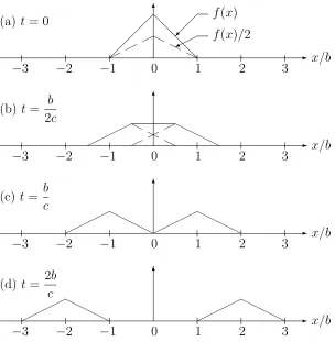
2[f(x−ct) +f(x+ct)], (3.22) which may be interpreted as two waves, each equal to f(x)/2, which travel at speed c to the right and left, respectively. For example, the argument x−ct remains constant if, as t increases,xalso increases at speed c. Thus, the wavef(x−ct) moves to the right (increasing x) with speed c without change of shape. Similarly, the wave f(x+ct) moves to the left (decreasing x) with speedcwithout change of shape. The two waves [each equal to half the initial shapef(x)] travel in opposite directions from each other at speedc. Iff(x) is nonzero only for a small domain, then, after both waves have passed the region of initial disturbance, the string returns to its rest position.

For example, let f(x), the initial displacement, be given by

f(x) =

−|x|+b, |x| ≤b,

0, |x| ≥b, (3.23)

which is a triangular pulse of width 2b and height b (Fig. 14). For t > 0, half this pulse travels in opposite directions from the origin. For t > b/c, where c is the wave speed, the two half-pulses have completely separated, and the neighborhood of the origin has returned to rest.

For the special case f(x) = 0 (zero initial displacement), the d’Alembert solution simpli-fies to

u(x, t) = 1 2c

Z x+ct

x−ct

g(τ)dτ = 1

2[G(x+ct)−G(x−ct)], (3.24) where

G(x) = 1 c

Z x −∞

g(τ)dτ. (3.25)

(31)

-6

x/b

−3 −2 −1 0 1 2 3

f(x)/2 f(x)

(a) t = 0 @

@ @

@ H

H H

-6

x/b

−3 −2 −1 0 1 2 3

(b) t = b 2c

H H

H H H

H H

-6

x/b

−3 −2 −1 0 1 2 3

(c) t = b c

H H H H

-6

x/b

−3 −2 −1 0 1 2 3

(d) t = 2b c

H H H H

[image:31.612.155.459.64.375.2]

H H H H

Figure 14: Propagation of Initial Displacement.

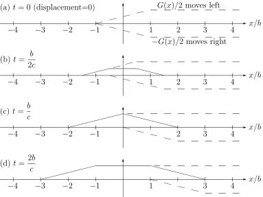
For example, let the initial velocity g(x) be given by

g(x) =

M c, |x|< b,

0, |x|> b, (3.26)

which is a rectangular pulse of width 2b and height M c, where the constant M is the dimensionless Mach number, and c is the wave speed (Fig. 15). The travelling wave G(x) is given by Eq. 3.25 as

G(x) =  



0, x≤ −b,

M(x+b), −b≤x≤b, 2M b, x≥b.

(3.27)

That is, half this wave travels in opposite directions at speedc. Even though g(x) is nonzero only near the origin, the travelling wave G(x) is constant and nonzero for x > b. Thus, as time advances, the center section of the string reaches a state of rest, but not in its original position (Fig. 16).

From the preceding discussion, it is clear that disturbances travel with speed c. For an observer at some fixed location, initial displacements occurring elsewhere pass by after a finite time has elapsed, and then the string returns to rest in its original position. Nonzero initial velocity disturbances also travel at speed c, but, once having reached some location, will continue to influence the solution from then on.

Thus, the domain of influence of the data at x =x0, say, on the solution consists of all

(32)

-6

x/b g(x)

−3 −2 −1 0 1 2 3

(a)

-6

x/b G(x)

−3 −2 −1 0 1 2 3

(b)

[image:32.612.114.497.362.649.2]

Figure 15: Initial Velocity Function.

-6

x/b

−4 −3 −2 −1 1 2 3 4

G(x)/2 moves left

−G(x)/2 moves right (a) t= 0 (displacement=0)

X X

-6

x/b

−4 −3 −2 −1 1 2 3 4

(b) t= b 2c

XXX

X

X X

-6

x/b

−4 −3 −2 −1 2 3 4

(c) t= b c

X X X X X X X X X

X X

X

-6

x/b

−4 −3 −2 −1 1 3 4

(d) t= 2b c

X X X X X X X X X

X X

X

(33)

-6

x t

r

@ @ @ @ @ @

slope=1/c

−1/c

(x0,0)

(a) Domain of Influence of Data on Solution.

-6

x t

r

@ @

@

−1/c 1/c

(x, t)

r r

(x−ct,0) (x+ct,0) (b) Domain of Dependence

of Solution on Data. Figure 17: Domains of Influence and Dependence.

Conversely, thedomain of dependence of the solution on the initial data consists of all points within a distance ct of the solution point. That is, the solution at (x, t) depends on the initial data for all locations in the range (x−ct, x+ct), which are the limits of integration in the d’Alembert solution, Eq. 3.20.

3.2.2 Finite Differences

From the preceding discussion of the d’Alembert solution, we see that hyperbolic equations involve wave motion. If the initial data are discontinuous (as, for example, in shocks), the most accurate and the most convenient approach for solving the equations is probably the method of characteristics. On the other hand, problems without discontinuities can probably be solved most conveniently using finite difference and finite element techniques. Here we consider finite differences.

Consider the boundary-initial value problem (BIVP) 

  

  

uxx =

1

c2 utt, u=u(x, t), 0< x < a, t >0

u(0, t) = u(a, t) = 0 (boundary conditions)

u(x,0) =f(x), ut(x,0) =g(x) (initial conditions).

(3.28)

This problem represents the transient (time-dependent) vibrations of a string fixed at the two ends with both initial displacementf(x) and initial velocityg(x) specified.

A central finite difference approximation to the PDE, Eq. 3.28, yields ui+1,j −2ui,j +ui−1,j

h2 =

ui,j+1−2ui,j+ui,j−1

c2_k2 . (3.29)

We define the parameter

r= ck h =

c∆t

∆x, (3.30)

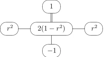
and solve for ui,j+1:

ui,j+1=r2ui−1,j+ 2(1−r2)ui,j+r2ui+1,j−ui,j−1. (3.31)

(34)

-6

x t

0 u=f(x), ut=g(x) a

u= 0 u= 0

s

i, j+1

s

i, j−1

h -? 6

[image:34.612.223.395.257.352.2]

k

Figure 18: Mesh for Explicit Solution of Wave Equation.

r2

2(1−r2₎

r2

1

−1

Figure 19: Stencil for Explicit Solution of Wave Equation.

all time values up to thejth time step, we can compute the solution ui,j+1 at Step j+ 1 in

terms of known quantities. Thus, this algorithm is an explicit algorithm. The corresponding stencil is shown in Fig. 19.

It can be shown that this finite difference algorithm is stable ifr ≤1 and unstable ifr >1. This stability condition is know as the Courant, Friedrichs, and Lewy (CFL) condition or simply the Courant condition. It can be further shown that a theoretically correct solution is obtained when r = 1, and that the accuracy of the solution decreases as the value of r decreases farther and farther below the value of 1. Thus, the time step size ∆t should be chosen, if possible, so that r = 1. If that ∆t is inconvenient for a particular calculation, ∆t should be selected as large as possible without exceeding the stability limit of r= 1.

An intuitive rationale behind the stability requirement r ≤ 1 can also be made using Fig. 20. If r > 1, the numerical domain of dependence (NDD) would be smaller than the actual domain of dependence (ADD) for the PDE, since NDD spreads by one mesh point at each level for earlier time. However, if NDD < ADD, the numerical solution would be independent of data outside NDD but inside ADD. That is, the numerical solution would ignore necessary information. Thus, to insure a stable solution, r≤1.

3.2.3 Starting Procedure for Explicit Algorithm

(35)

-6

x t

-h

? 6_k

s

@ @

@ @ #

# # # # # # # # # # # #

c c

c

Numerical Domain of Dependence

-Actual Domain of Dependence

-Slope = 1/c

Z

~ Slope = −1/c

Figure 20: Domains of Dependence for r >1.

The explicit finite difference algorithm is given in Eq. 3.31:

To compute the solution at the end of the first time step, letj = 0:

ui,1 =r2ui−1,0+ 2(1−r2)ui,0+r2ui+1,0 −ui,−1, (3.33)

where the right-hand side is known (from the initial condition) except for ui,−1. However,

we can write a central difference approximation to the first time derivative at t= 0: ui,1 −ui,−1

2k =gi (3.34)

or

ui,−1 =ui,1−2kgi, (3.35)

wheregiis the initial velocityg(x) evaluated at theith point, i.e.,gi =g(xi). If we substitute

this last result into Eq. 3.33 (to eliminateui,−1), we obtain

ui,1 =r2ui−1,0+ 2(1−r2)ui,0+r2ui+1,0−ui,1+ 2kgi (3.36)

or

ui,1 =

1 2r

2

ui−1,0+ (1−r2)ui,0+

1 2r

2

ui+1,0+kgi. (3.37)

This is the difference equation used for the first row. Thus, to implement the explicit finite difference algorithm, we use Eq. 3.37 for the first time step and Eq. 3.31 for all subsequent time steps.

3.2.4 Nonreflecting Boundaries

(36)

s s s

s

c c s c c

i, j

Figure 21: Finite Difference Mesh at Nonreflecting Boundary.

to be truncated at some sufficiently large distance. At such a boundary, a suitable boundary condition must be imposed to ensure that outgoing waves are not reflected.

Consider a vibrating string which extends to infinity for largex. We truncate the compu-tational domain at some finite x. Let the initial velocity be zero. The d’Alembert solution, Eq. 3.20, of the one-dimensional wave equation c2uxx =utt can be written in the form

u(x, t) = F1(x−ct) +F2(x+ct), (3.38)

where F1 represents a wave advancing at speed c toward the boundary, and F2 represents

the returning wave, which should not exist if the boundary is nonreflecting. With F2 = 0,

we differentiateu with respect to x and t to obtain ∂u

∂x =F 0

1,

∂u

∂t =−cF 0

1, (3.39)

where the prime denotes the derivative with respect to the argument. Thus, ∂u

∂x =− 1 c

∂u

∂t. (3.40)

This is the one-dimensional nonreflecting boundary condition. Note that the x direction is normal to the boundary. The boundary condition, Eq. 3.40, must be imposed to inhibit reflections from the truncated boundary. This condition is exact in 1-D (i.e., plane waves) and approximate in higher dimensions, where the nonreflecting condition is written

c∂u ∂n+

∂u

∂t = 0, (3.41)

where n is the outward unit normal to the boundary.

The nonreflecting boundary condition, Eq. 3.40, can be approximated in the finite dif-ference method with central difdif-ferences expressed in terms of the phantom point outside the boundary. For example, at the typical point (i, j) on the nonreflecting boundary in Fig. 21, the general recursive formula is given by Eq. 3.31:

The central difference approximation to the nonreflecting boundary condition, Eq. 3.40, is

cui+1,j−ui−1,j

2h =−

ui,j+1−ui,j−1

(37)

or

r(ui+1,j−ui−1,j) =−(ui,j+1−ui,j−1). (3.44)

The substitution of Eq. 3.44 into Eq. 3.42 (to eliminate the phantom point) yields

(1 +r)ui,j+1 = 2r2ui−1,j+ 2(1−r2)ui,j−(1−r)ui,j−1. (3.45)

For the first time step (j = 0), the last term in this relation is evaluated using the central difference approximation to the initial velocity, Eq. 3.35. Note also that, for r= 1, Eq. 3.45 takes a particularly simple (and perhaps unexpected) form:

ui,j+1 =ui−1,j. (3.46)

To illustrate the perfect wave absorption that occurs in a one-dimensional finite difference model, consider an infinitely-long vibrating string with a nonzero initial displacement and zero initial velocity. The initial displacement is a triangular-shaped pulse in the middle of the string, similar to Fig. 14. According to the d’Alembert solution, half the pulse should propagate at speed c to the left and right and be absorbed into the boundaries. We solve the problem with the explicit central finite difference approach with r = ck/h = 1. With r= 1, the finite difference formulas 3.31 and 3.37 simplify to

ui,j+1 =ui−1,j+ui+1,j−ui,j−1 (3.47)

and

ui,1 = (ui−1,0+ui+1,0)/2. (3.48)

On the right and left nonreflecting boundaries, Eq. 3.46 implies

un,j+1 =un−1,j, u0,j+1 =u1,j, (3.49)

where the mesh points in the xdirection are labeled 0 ton. The finite difference calculation for this problem results in the following spreadsheet:

(38)

ρcA @ @ @

Figure 22: Finite Length Simulation of an Infinite Bar.

Notice that the triangular wave is absorbed without any reflection from the two boundaries. For steady-state wave motion, the solution u(x, t) is time-harmonic, i.e.,

u=u0eiωt, (3.50)

and the nonreflecting boundary condition, Eq. 3.40, becomes ∂u0

∂x =− iω

c u0 (3.51)

or, in general,

∂u0

∂n =− iω

c u0 =−iku0, (3.52)

where n is the outward unit normal at the nonreflecting boundary, and k = ω/c is the wave number. This condition is exact in 1-D (i.e., plane waves) and approximate in higher dimensions.

The nonreflecting boundary condition can be interpreted physically as a damper (dash-pot). Consider, for example, a bar undergoing longitudinal vibration and terminated on the right end with the nonreflecting boundary condition, Eq. 3.40 (Fig. 22). The internal longitudinal force F in the bar is given by

F =Aσ=AEε=AE∂u

∂x, (3.53)

where A is the cross-sectional area of the bar, σ is the stress, E is the Young’s modulus of the bar material, and u is displacement. Thus, from Eq. 3.40, the nonreflecting boundary condition is equivalent to applying an end force given by

F =−AE

c v, (3.54)

where v =∂u/∂t is the velocity. Since, from Eq. 2.10,

E =ρc2, (3.55)

Eq. 3.54 becomes

F =−(ρcA)v, (3.56)

(39)

-6

x y

a b

T =f1(x)

T =f2(x)

T =g1(y) ∇2T = 0 T =g2(y)

Figure 23: Laplace’s Equation on Rectangular Domain.

-6

s Point (i, j)

i−1 i i+ 1 j−1

j j+ 1

Figure 24: Finite Difference Grid on Rectangular Domain.

3.3 Elliptic Equations

Consider Laplace’s equation on the two-dimensional rectangular domain shown in Fig. 23:

∇2_T_{(x, y) = 0} ₍₀_{< x < a,} ₀_{< y < b),}

T(0, y) =g1(y), T(a, y) =g2(y), T(x,0) =f1(x), T(x, b) =f2(x).

(3.57)

This problem corresponds physically to two-dimensional steady-state heat conduction over a rectangular plate for which temperature is specified on the boundary.

We attempt an approximate solution by introducing a uniform rectangular grid over the domain, and let the point (i, j) denote the point having theith value of xand the jth value of y(Fig. 24). Then, using central finite difference approximations to the second derivatives (Fig. 25),

∂2_T

∂x2 ≈

Ti−1,j−2Ti,j+Ti+1,j

h2 , (3.58)

∂2_T

∂y2 ≈

Ti,j−1−2Ti,j+Ti,j+1

h2 . (3.59)

The finite difference approximation to Laplace’s equation thus becomes Ti−1,j−2Ti,j +Ti+1,j

h2 +

Ti,j−1−2Ti,j +Ti,j+1

h2 = 0 (3.60)

or

(40)

s

h

-6

?

h

(i−1, j−1) (i, j−1) (i+ 1, j−1) (i−1, j) (i, j) (i+ 1, j) (i−1, j+ 1) (i, j+ 1) (i+ 1, j+ 1)

Figure 25: The Neighborhood of Point (i, j).

1 2 3 4

5 6 7 8

9 10 11 12

13 14 15 16

17 18 19 20

Figure 26: 20-Point Finite Difference Mesh.

That is, for Laplace’s equation with the same uniform mesh in each direction, the solution at a typical point (i, j) is the average of the four neighboring points.

For example, consider the mesh shown in Fig. 26. Although there are 20 mesh points, 14 are on the boundary, where the temperature is known. Thus, the resulting numerical problem has only six degrees of freedom (unknown variables). The application of Eq. 3.61 to each of the six interior points yields

        

       

4T6 − T7 − T10 = T2+T5

−T6 + 4T7 − T11 = T3+T8

−T6 + 4T10 − T11 − T14 = T9

−T7 − T10 + 4T11 − T15 = T12

−T10 + 4T14 − T15 = T13+T18

−T11 − T14 + 4T15 = T16+T19,

(3.62)

(41)

-6

x y

a b

T =f1(x)

T =f2(x)

T =g1(y)

∂T

∂x =g(y)

∇2_T _{= 0}

Figure 27: Laplace’s Equation With Dirichlet and Neumann B.C.

Since the numbers assigned to the mesh points in Fig. 26 are merely labels for identifica-tion, the pattern of nonzero coefficients appearing on the left-hand side of Eq. 3.62 depends on the choice of mesh ordering. Some equation solvers based on Gaussian elimination oper-ate more efficiently on systems of equations for which the nonzeros in the coefficient matrix are clustered near the main diagonal. Such a matrix system is called banded.

Systems of this type can also be solved using an iterative procedure known as relaxation, which uses the following general algorithm:

1. Initialize the boundary points to their prescribed values, and initialize the interior points to zero or some other convenient value (e.g., the average of the boundary values). 2. Loop systematically through the interior mesh points, setting each interior point to

the average of its four neighbors.

3. Continue this process until the solution converges to the desired accuracy.

3.3.1 Derivative Boundary Conditions

The approach of the preceding section must be modified for Neumann boundary conditions, in which the normal derivative is specified. For example, consider again the problem of the last section but with a Neumann, rather than Dirichlet, boundary condition on the right side (Fig. 27):

 



∇2_T_{(x, y) = 0} ₍₀_{< x < a,} ₀_{< y < b),}

T(0, y) = g1(y),

∂T(a, y)

∂x =g(y), T(x,0) =f1(x), T(x, b) = f2(x).

(3.63)

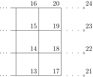
We extend the mesh to include additional points to the right of the boundary at x = a (Fig. 28). At a typical point on the boundary, a central difference approximation yields

g18 =

∂T18

∂x ≈

T22−T14

2h (3.64)

or

T22 =T14+ 2hg18. (3.65)

On the other hand, the equilibrium equation for Point 18 is

(42)

. . . . . . . . . . . .

p p p b p p p b p p p b p p p b

13 14 15 16

17 18 19 20

21 22 23 24

Figure 28: Treatment of Neumann Boundary Conditions.

AAAA

k1

m2

- u₂(t)

e e AAAA

k2

m3

- u₃(t)

e e

[image:42.612.223.387.83.219.2]

- f₃(t)

Figure 29: 2-DOF Mass-Spring System.

which, when combined with Eq. 3.65, yields

4T18−2T14−T17−T19= 2hg18, (3.67)

which imposes the Neumann boundary condition on Point 18.

4 Direct Finite Element Analysis

The finite element method is a numerical procedure for solving partial differential equations. The procedure is used in a variety of applications, including structural mechanics and dy-namics, acoustics, heat transfer, fluid flow, electric and magnetic fields, and electromagnetics. Although the main theoretical bases for the finite element method are variational principles and the weighted residual method, it is useful to consider discrete systems first to gain some physical insight into some of the procedures.

4.1 Linear Mass-Spring Systems

Consider the two-degree-of-freedom (DOF) system shown in Fig. 29. We let u2 and u3

denote the displacements from the equilibrium of the two massesm2 andm3. The stiffnesses

of the two springs arek1 andk2. The dynamic equilibrium equations could be obtained from

Newton’s second law (F=ma):

m2u¨2+k1u2−k2(u3−u2) = 0

m3u¨3+k2(u3−u2) = f3(t)

(43)

AAAA

k

c c

[image:43.612.72.536.62.460.2]

1 2

Figure 30: A Single Spring Element.

or

m2u¨2+ (k1 +k2)u2−k2u3 = 0

m3u¨3−k2u2 +k2u3 = f3(t).

(4.2)

This system could be rewritten in matrix notation as

M¨u+Ku=F(t), (4.3)

where

u=

u2

u3

(4.4)

is the displacement vector (the vector of unknown displacements),

K=

k1+k2 −k2 −k2 k2

(4.5)

is the system stiffness matrix,

M=

m2 0

0 m3

(4.6)

is the system mass matrix, and

F=

0 f3

(4.7)

is the force vector. This approach would be very tedious and error-prone for more complex systems involving many springs and masses.

To develop instead a matrix approach, we first isolate one element, as shown in Fig. 30. The stiffness matrix Kel for this element satisfies

Kelu=F, (4.8)

or

k11 k12

k21 k22

u1

u2

=

f1

f2

. (4.9)

By expanding this equation, we obtain

k11u1+k12u2 =f1

k21u1+k22u2 =f2

. (4.10)

From this equation, we observe thatk11 can be defined as the force on DOF 1 corresponding

to enforcing a unit displacement on DOF 1 and zero displacement on DOF 2:

k11 =f1

(44)

AAAA

k1

AAAA

k2

c c c

1 2 3

Figure 31: 3-DOF Spring System.

Similarly,

k12 =f1

u1=0,u2=1 =−k, k21=f2

u1=1,u2=0 =−k, k22 =f2

u1=0,u2=1 =k. (4.12)

Thus,

Kel =

k −k

−k k

=k

1 −1

−1 1

. (4.13)

In general, for a larger system with many more DOF,

K11u1+K12u2+K13u3+· · ·+K1nun=F1

K21u1+K22u2+K23u3+· · ·+K2nun=F2

K31u1+K32u2+K33u3+· · ·+K3nun=F3

.. .

Kn1u1+Kn2u2+Kn3u3+· · ·+Knnun=Fn

      

     

, (4.14)

in which case we can interpret an individual element Kij in the stiffness matrix as the force

at DOF i if uj = 1 and all other displacement components ui = 0:

Kij =Fi

uj=1,others=0. (4.15)

4.2 Matrix Assembly

We now return to the stiffness part of the original problem shown in Fig. 29. In the absence of the masses and constraints, this system is shown in Fig. 31. Since there are three points in this system, each with one DOF, the system is a 3-DOF system. The system stiffness matrix can be assembled for this system by adding the 3×3 stiffness matrices for each element:

K= 



k1 −k1 0 −k1 k1 0

0 0 0



+ 



0 0 0

0 k2 −k2

0 −k2 k2



= 



k1 −k1 0 −k1 k1+k2 −k2

0 −k2 k2



. (4.16)

The justification for this assembly procedure is that forces are additive. For example, k22 is

the force at DOF 2 when u2 = 1 and u1 =u3 = 0; both elements which connect to DOF 2

contribute to k22. This matrix corresponds to the unconstrained system.

4.3 Constraints

(45)

AAAA

k1

AAAA

k2

r c c

1 2 3

fixed

Figure 32: Spring System With Constraint.

AAAA

k1

AAAA

k2

AAAA

k4

AAAA

k3

c

c c

1

2

3 4

Figure 33: 4-DOF Spring System.

(unconstrained) matrix system Ku=Finto

K11u1+K12u2+K13u3 =F1

K21u1+K22u2+K23u3 =F2

K31u1+K32u2+K33u3 =F3

 



, (4.17)

we see that Row i corresponds to the equilibrium equation for DOF i. Thus, if ui = 0,

we do not need Row i of the matrix (although that equation can be saved to recover later the constraint force). Also, Column i of the matrix multiplies ui, so that, if ui = 0, we do

not need Column i of the matrix. That is, if ui = 0 for some system, we can enforce that

constraint by deleting Row i and Column i from the unconstrained matrix. Hence, with u1 = 0 in Fig. 32, we delete Row 1 and Column 1 in Eq. 4.16 to obtain the reduced matrix

K=

k1+k2 −k2 −k2 k2

, (4.18)

which is the same matrix obtained previously in Eq. 4.5. Notice that, from Eqs. 4.16 and 4.18,

detK3×3 =k1[(k1+k2)k2−k22] +k1(−k1k2) = 0, (4.19)

whereas

detK2×2 = (k1 +k2)k2−k22 =k1k2 6= 0. (4.20)

That is, the unconstrained matrix K3×3 is singular, but the constrained matrix K2×2 is

nonsingular. Without constraints, Kis singular (and the solution of the mechanical problem is not unique) because of the presence of rigid body modes.