A Time Dependent Pollution Routing Problem in Multi-graph

(1)

Please cite this article as: M. Setak, Z. Shakeri, A. Patoghi, A Time Dependent Pollution Routing Problem in Multi-graph, International Journal of Engineering (IJE), TRANSACTIONSB: Applications Vol. 30, No. 2, (February 2017) 234-242

International Journal of Engineering

J o u r n a l H o m e p a g e : w w w . i j e . i r

A Time Dependent Pollution Routing Problem in Multi-graph

M. Setak*_{, Z. Shakeri, A. Patoghi}

Department of Industrial Engineering, K. N. Toosi University of Technology, Tehran, Iran

P A P E R I N F O

Paper history:

Received 08 November 2016

Received in revised form 23 December 2016 Accepted 05 January 2017

Keywords: Time – dependent Pollution Routing Problem Multi-graph

Tabu Search

A B S T R A C T

This paper considers a time dependent (the travel time is not constant throughout the day) pollution routing problem (TDPRP), which aids the decision makers in minimizing travel time, toll cost and emitted pollution cost. In complexity of urban areas most of the time one point is accessible from another with more than one edge. In contrast to previous TDPRP models, which are designed with only one edge between two nodes, the existence of more than one edge between two nodes is allowed in our modeling. Thus we develop a new model that is called time dependent pollution routing problem in multi-graph (TDPRPM). Since the problem is NP-hard, a tabu search (TS) algorithm is developed to solve it. Finally, computational results of tabu search procedure and its comparison to exact solution are presented.

doi: 10.5829/idosi.ije.2017.30.02b.10

1. INTRODUCTION1

The modern economic environment is gaining far reaching complexity and completion. All business sectors are facing a lot of pressure for cost reduction in order to survive in this competitive environment. Logistics is the main part of supply chain management playing a significant role in cost reduction. Logistics management plans, implement and control the efficient, effective forward and reverse flow and storage of goods, services, and related information between the point of origin and the point of consumption in order to meet customer's requirements. Among these activities transportation planning or in other words planning for efficient transfer of goods or people between desired locations by a fleet of vehicles through communication networks is very critical. Problems related to the distribution of goods between the warehouse and the final customer is generally considered as vehicle routing problem (VRP).

Vehicle routing problem was first raised by Dantzig and Ramser [1]. Afterwards, Clarke and Wright [2] improved an algorithm for problems with more than two vehicles. Gradually some assumptions such as discussing time dependency, considering more than one

1_{*Corresponding Author’s Email:}_{Setak@kntu.ac.ir}_{(M. Setak)}

path between two nodes or taking into account released pollution were added to the classical vehicle routing problem.

(2)

between two nodes was depended on the departure time. In the work presented by Huart et al. [10] a time dependent vehicle routing problem with time windows was studied. They supposed a specific speed for each arcand finally a Dijkstra algorithm was adapted for determining the shortest path. Figliozzi [11] considered the route and the travel time as decision variables, thereafter in another work [12], he presented a model for optimizing speed of vehicles.

In the vehicle routing problem, it is assumed that there is only one edge between two nodes, however due to the complexity of urban areas it is clear that most of the time there is more than one path between two nodes. Moreover, there are circumstances in which traffic congestion forces decision makers to create a new path between nodes in order to reduce cost of emissions, travel time, and driver. To the best of our knowledge for the first time Setak et al. [13] discussed vehicle routing problem in a multi-graph network with FIFO priority. Huang et al. [14] developed a time dependent VRP with path flexibility (existence of multiple paths between two nodes). Moreover, they formulated their model under deterministic and stochastic traffic conditions. Garaix et al. [15] studied the consideration of alternative paths and evaluated their impact on solution algorithm through a multi graph network.

Regarding to the importance of the vehicle routing problem and its effects on the environment such as greenhouse gas emissions and its harms to human’s health; a new branch of VRP was introduced by Bektas and Laporte [16] as pollution routing problem (PRP). Considering the pollution in the vehicle routing is an extension of the classical VRP, so that instead of discussing the traveled distance, it discusses the amount of greenhouse gas emissions, fuel consumption and the travel time. There are several studies in the literature related to fuel consumption and emissions. Apaydin and Gonullu [17] tried to control emissions in the context of route optimization with a constant emission factor to estimate fuel consumption. Kuo [18] discussed the fuel consumption depending on transportation speed and load of the vehicle and tried to minimize it in a time dependent vehicle routing problem. Jabali et al. [19] also studied a time dependent VRP which its aim was to minimize CO2 emissions. Their model was solved via tabu search algorithm.

Suzuki [20] calculated fuel consumption by considering load, speed of the vehicle, slope of the road and vehicle’s waiting time. Kramer et al. [21] proposed a time window pollution routing problem with vehicle capacity constraint. In their modeling costs were based on driver wages and fuel consumption wherein vehicle’s load and travel distance were involved in calculation. Wen and Eglese [22] introduced LANCOST heuristic approach for solving vehicle routing and scheduling problem to minimize the total travel cost, which consists of fuel cost, driver wages and congestion cost. Fuel

consumption depends on the vehicle speed and the speed is influenced by the congestion, more over if a vehicle enters a congestion charge zone it should pay a fixed charge. Qian and Eglese [23] presented a model which determines routes for a fleet of delivery vehicles with consideration of minimum fuel emissions. The speed of vehicle through each road is also considered as decision variable. A column generation based tabu search algorithm was applied to solve the problem. Kramer et al. [24] introduced a new speed and departure time optimization algorithm for the pollution routing problem. In Kramer modeling in order to reduce the CO2 emission, vehicles were allowed to leave the depot with delay. According to the literature and to the best of our knowledge there has been no attention toward time dependent pollution routing problem in multi-graph. Overall the main contributions of this paper are as follows:

 Discussing pollution emissions

 Proposing network of routes as a multi-graph network where there are more than one edge between two nodes

 Considering a specific toll for each edge

Such considerations make this study unique and advantages in reflecting complexity of urban areas.

The rest of this paper is organized as follows: In section 2, time dependent PRP in multi-graph is described and is modeled using linear integer programming. Since the problem is NP-hard a tabu search procedure is applied to solve the problem in section 3. In section 4 computational results are presented for some examples.

2. PROBLEM FRAMEWORK

The main purpose of this paper is to minimize the amount of pollution that is emitted by vehicles and also to reduce other costs relating to the time of travel and traffic condition. The following assumptions are considered in the model:

1. All the vehicles leave the depot at the same time. 2. After visiting the last customer all the vehicles

return to the depot.

3. All customers’ demand is fixed and known. 4. Fleet vehicles are homogenous with fixed and

determined capacity.

5. The number of vehicles is determined.

6. Each customer is given service only by a vehicle. 7. The main objective of the model is to reduce the

emitted pollution.

8. A specific toll is defined for each edge.

(3)

2. 1. TDPRPM Model In this section first we introduce the following assumptions and notations which are used in our mixed integer linear programming. Thereafter, based on the aforementioned assumptions and described parameters and variables we develop our TDPRPM model. In Table 1 parameters, variables and sets are introduced. Suppose G= (V, E) as a complete graph, in which V is the set of nodes and E is the set of edges. Each edge can be defined by a regular ternary as( , , , l )

ij

i j mij .

Here

i

is the origin node, j is the destination node, ij

m

indicates mth edge between two aforementioned nodes and lij defines 𝑙𝑡ℎ time interval from node 𝑖 to node𝑗.

Following formulation is used to calculate the amount of needed energy to move through mthedge from node

i

to node j [16].

2

( ) d

mij

P W w_ij V_mlijd_mij

mij mij

 

  

mij

 _{is arc specific constant which is calculated as the}

following formulation and depends on each arc angle

and vehicles’ acceleration.



a gsin( _mij) g Cr cos( _mij)



mij



  



     



is vehicle specific constant and due to the homogenous transportation system in our study is identical for all vehicles.



0.5 Cd A





 



    

Figure 1. Representation of simple graph (A) vs. multi-graph (B) (Setak et al. [13]).

TABLE 1. Parameters and variables of model

Sets mij Arc specific constant (m/s

2

*g/j)

L Set of time intervals (𝑙 ∈ 𝐿)  Vehicle specific constant (kg/m*g/j))

M Set of arcs between two nodes (m ∈ M) mij Slope of mth edge between nodes i and j

V Set of nodes (𝑖, 𝑗 ∈ 𝑉 and 𝑖 = 0 indicates the depot) Cr Coefficients of rolling resistance

Parameters Cd Coefficients of drag

i

S Service time for customer

i

(s) A Frontal surface area of the vehicle (m2₎

K The number of vehicles



Air density (kg/m3₎

G Capacity of vehicle (kg) a Acceleration (m/s2₎

i

q

Demand of customer

i

(q0=0) (kg)  Fuel to air mass ratio

p Driver wages per unit time ($/s)  Heating value of a typical diesel fuel (j/g)

mij

C Toll cost of mth edge between

i

and j ($) MM Large number

E Fix cost of vehicle ($) BB Large number

mij

d _{Distance between two}_i_and_j_{nodes of the mth edge (m)} Variables

mlij

v Speed of the vehicle from node i to node j of mth edge in the lth

time interval (m/s)

x

mlij

1 if the vehicle moves from node i to node j of mth edge

in the lth time interval otherwise 0

ij

u Upper bound of lth time interval between node i and j (s) b_i Departure time from node i (s)

c

f Fuel consumption cost per unit ($/g) Fj Total traveled time when node 𝑖 is the last visited node (s)

W Weight of the vehicle (with no freight) (kg)

w

_ij Amount of freight carried by a vehicle from node i to

node j (kg)

g Gravitational constant (9.81 m/s2₎

(e,d)

(e,d,1) (e,d,2) d

e

a b a b

c _c

(4)

Below, the formulation of TDPRPM is presented:

0 0 1 1

0 0 1

2

0 0 1 1

( ( ) ) mij mij mij ij M L N N mij mlij

i j m l

M N N

ij mij

i j m

L M

N N

mij mlij mlij

i j l m

Min fc d x W

w d

d v x

Z

                









(1.a) Subject to: 0 1 1 1

M L N

ml j

m l j

0 0, 0

i

w   i (10)

0 0

b  (11)

( ) (1 )

1 1 1 1

, 1, ..., . , 1, ..., . d

L M _mij L M

b b s x MM x

i j j mlij mlij

l m l m

v mlij

i j N i j N

                  (12) 0 0 0

1 1 1 1

0

( ) (1 )

1, ...,

,

L M L M

mi

j j mlj mlj

l m l m

mli

d

b F x MM x

v

j

N

        

 

 

(13) (1 ),

, 1, ..., ( ).

1, ..., . 1, ..., .

i lij mlij

b u BB x

i j N i j

l L m M

  

  

   

(14)

( 1) 0, , 1, ..., ( ).

1, ..., . 1, ..., .

i l ij mlij

b u x i j N i j

l L m M



     

    (15)

0 1, , 1,..., ( ).

1,..., . 1,..., .

mlij

x or i j N i j

l L m M

   

    (16)

, , 0,

, 1,..., ( ).

1,..., . 1,..., .

i ij j

b w F

i j N i j

l L m M



  

   

(17)

The objective function (1) includes minimizing: (1.a) the cost of consumed energy; it is clear that a reduction in the consumed energy will reduce the emitted pollution which is one of the main concerns of this study; (1.b) cost related to driver wages (each driver wage is calculated based on total travel time); (1.c) vehicle acquisition cost and (1.d) toll cost; it should be noted that the toll cost of paths differ from one path to another according to the traffic congestion or the length of each path. Constraints (2) and (5) express that the number of departure from the depot and the number of arrival to the depot are the same. Constraints (3) and (4) ensure that each node is visited exactly once. It is guaranteed in constrain (6) that loading from the depot is less than vehicles capacity. Constraint (7) indicates that when a vehicle passes an arc from node 𝑖 to node𝑗, its freight must meet the demand of node𝑗. If a vehicle meets node 𝑖 its freight must be as much as the difference between the total capacity and the demand of node 𝑖; this subject is investigated in constraint (8). Constraint (9) ensures that the difference between the j

j pF





_(1.b)

0 0 0 1

M

N L

mli

i l m

E x

  

 



(1.c)

0 0 1 1

M

N N L

mij mlij

i j m l

C x

   

(5)

load carried to node 𝑖 and the load extracted from this node is equal to the node's demanding amount. Constraint (10) indicates that the vehicle returns to the depot empty. Constraint (11) shows the departure time from depot. Constraint (12) determines the departure time from customer nodes and constraint (13) indicates the total travel time. Constraints (14) and (15) state the time intervals of the departure of vehicles. According to Constraint (14) if the departure time is lower than the upper bound of 𝑙𝑡ℎ time interval and according to Constraint (15) if it is upper than the upper bound of

(𝑙 − 1)𝑡ℎ time interval, then definitely the departure time is in the 𝑙𝑡ℎ time interval. Constraints (16) and (17) represent the type of variables.

3. THE PROPOSED TABU SEARCH ALGORITHM

In the VRP with the increase of problem scale the solution time increases non-polynomially using exact solvers. Moreover, many studies such as Fakhri and Sadri Esfahani [25] have proved tabu search procedure efficiency in VRP issues. Hence, a tabu search algorithm is used to solve the problem in less computational time. The proposed tabu search algorithm is explained and its results are presented in the following.

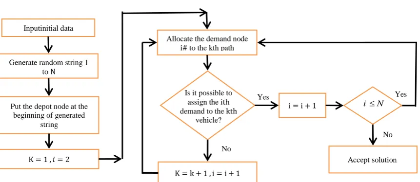
3. 1. Feasibility of a Soulotion To determine an initial solution, first a sequence of customer visiting is provided. With consideration of vehicle capacity and customers demand, each customer is allocated to a vehicle in which all the customers receive service. In Figure 2 the process for producing the feasible solution is shown.

3. 2. Objective Function The objective function is a cost minimization function that consists of four terms. First part is related to the cost of energy consumption. In the second part there is driver cost which is calculated by computing the total travel time. The third part indicates vehicles cost and the final part concerns about toll cost.

3. 3. TABU Search Parameters The proposed tabu search algorithm consists of three main parameters: the length of tabu list, tabu tenure and maximum number of iteration. According to Setak et al. the tabu list length is N(N-1)/2, in which N is the number of nodes. Based on Taguchi analysis that is implemented on an example with five levels for tabu tenure (N/12, N/6, N/3, N/2, 3N/2) and five levels for the maximum level of the iterations (10N, 12N, 14N, 16N, 18N). Finally N/3 and 14N are gained for the tabu tenure and the maximum level of iterations.

3. 4. Neighborhood Search In each iteration of the proposed TS algorithm neighborhoods are investigated N(N-1)/2 times. As a result, all the possible combinations are examined. The neighborhood search is randomly applied amongst swap and reverse strategies.

3. 5. The Proposed TABU Search Structure The structure of the proposed TS algorithm is as follows. First an initial solution is generated and its feasibility is checked. At the first stage this solution is the best solution with the lowest cost. Afterwards nodes are selected randomly for exchange. Exchanges are done based on Swap and Reverse strategies unless they are not in tabu list.

Figure 2. The process of producing a feasible solution Inputinitial data

Generate random string 1 to N

K = 1 , 𝑖 = 2

Put the depot node at the beginning of generated

string

K = k + 1 , i = i + 1

Allocate the demand node

i# to the kth path

i = i + 1

Accept solution No

Yes Is it possible to

assign the ith

demand to the kth

vehicle?

i N

Yes

(6)

Swap strategy is to choose two nodes of a sequence and swap their position without any change in other nodes sequence. In the Reverse strategy in addition to the change in position of two selected nodes, the sequence of the nodes between two aforementioned nodes will be reversed.

The cost function of the new solution is competed and compared with the pervious solution. The solution which has the minimum cost is considered as the best solution. Next three aforementioned TS parameters are updated and the process is continued until the maximum number of iterations.

4. COMPUTATIONAL RESULT

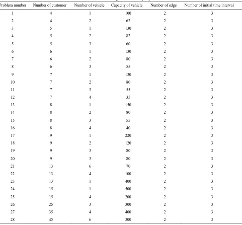
The twenty eight generated problems with different number of vehicles, different capacity and different number of customers is investigated (Table 2). These samples are solved by CPLEX 12 solver in GAMS 24.1.2 and the proposed Tabu search in Matlab on a system with CPU core i5, 2.6 GHz and 4.00 GB of ram. The results of two aforementioned procedures are shown in Table 3. The second column and the third one indicate Gams’ results and its computational time, respectively.

TABLE 2. Features of generated sample problem

Problem number Number of customer Number of vehicle Capacity of vehicle Number of edge Number of initial time interval

1 4 1 100 2 3

2 4 2 62 2 3

3 5 1 130 2 3

4 5 2 82 2 3

5 5 3 60 2 3

6 6 1 130 2 3

7 6 2 80 2 3

8 6 3 55 2 3

9 7 1 130 2 3

10 7 2 80 2 3

11 7 3 55 2 3

12 7 4 35 2 3

13 8 1 150 2 3

14 8 2 80 2 3

15 8 3 55 2 3

16 8 4 40 2 3

17 9 1 220 2 3

18 9 2 120 2 3

19 9 3 80 2 3

20 9 3 80 2 3

21 13 6 70 2 3

22 13 4 100 2 3

23 13 1 400 2 3

24 15 1 500 2 3

25 15 4 200 2 3

26 25 3 300 2 3

27 35 4 400 2 3

(7)

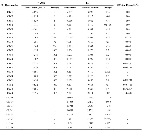
TABLE 3. The results of TS algorithm vs. CPLEX solver

Problem number

GAMS TS

RPD for TS results % Best solution (10^13) Time (s) Best solution Mean of solution Time (s)

C4V1 4.895 1 4.895 4.895 0.33 0.00

C4V2 4.915 1 4.915 4.915 0.05 0.00

C5V1 6.039 6 6.039 6.062 0.14 0.00

C5V2 6.111 5 6.111 6.119 0.1125 0.00

C5V3 6.161 1 6.161 6.161 0.15 0.00

C6V1 7.188 107 7.188 7.195 0.17 0.00

C6V2 7.265 100 7.295 7.306 0.32 0.4143

C6V3 7.361 92 7.361 7.369 0.21 0.0000

C7V1 8.165 310 8.165 8.203 0.13 0.0000

C7V2 8.154 1000 8.154 8.176 0.2 0.0000

C7V3 8.273 1001 8.273 8.303 0.2 0.0000

C7V4 8.382 1060 8.382 8.397 0.38 0.0000

C8V1 9.372 1001 9.391 9.424 0.3 0.198464

C8V2 9.474 1001 8.487 9.356 0.6 0.104159

C8V3 9.601 1001 9.601 9.618 0.991 0

C8V4 9.809 1000 9.809 9.920 0.8 0

C9V1 9.610 1000 9.629 9.656 0.8 0.198751

C9V2 9.632 1070 9.671 9.688 0.53 0.401786

C9V3 9.685 1000 9.710 9.742 0.6 0.256066

C9V4 9.756 1003 9.801 9.814 1.07 0.46228

C13V6 - - 1.6062 1.4343 1.4275

-C13V4 - - 1.4085 1.4172 1.5075

-C13V1 - - 1.3944 1.4005 1.38

-C15V1 - - 1.0499 1.1513 1.59

-C15V4 - - 1.3398 1.3527 1.471

-C25V3 - - 1.411 1.8959 2.0225

-C35V4 - - 1.25 1.5469 2.785

-C45V6 - - 2.02 2.9 3.011

-Columns 4-6 show results of proposed TS algorithm that are the best solution mean of solution and computational time. These results illustrate that the computational time by the CPLEX solver increases with the size growth of the problem severely. Furthermore, it’s not possible to reach an exact solution in many cases of the larger problems. Based on the literature VRP problems are NP- hard (Toth and Vigo [26]). In this paper a TDPRPM is investigated which is a more complex case than VRP, therefor this problem is NP-hard as well. Comparison of the results of the CPLEX solver and the proposed TS algorithm demonstrates the efficiency and the effectiveness of the TS algorithm. In the problems in which GAMS procures an exact solution, this algorithm obtains the identical result at all

running times. Different results are observed by increase of the number of customers. However, the quality of the TS solution is more proper in many of the cases, in which GAMS is not able to acquire the exact solution. The quality of the proposed TS algorithm is shown by calculating RPD index (Setak et al. [13]).

(8)

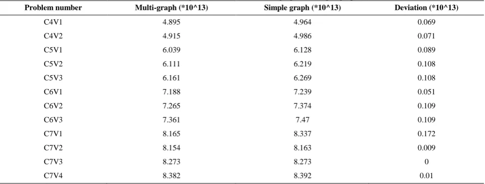
TABLE 4. The objective function of multi-graph vs. simple graph

Problem number Multi-graph (*10^13) Simple graph (*10^13) Deviation (*10^13)

C4V1 4.895 4.964 0.069

C4V2 4.915 4.986 0.071

C5V1 6.039 6.128 0.089

C5V2 6.111 6.219 0.108

C5V3 6.161 6.269 0.108

C6V1 7.188 7.239 0.051

C6V2 7.265 7.374 0.109

C6V3 7.361 7.47 0.109

C7V1 8.165 8.337 0.172

C7V2 8.154 8.163 0.009

C7V3 8.273 8.273 0

C7V4 8.382 8.392 0.01

As expected the objective function in the case of multi- graph is much better than the case of simple graph .This privilege signifies less cost of emissions, travel time, and driver. There are circumstances in which traffic congestion forces decision makers to create a new path between nodes in order to reduce cost of emissions, travel time, and driver. Consequently, the results of this study can be a means for urban decision makers to make the optimum decision on the selection of proper nodes for adding an extra edge or edges between them.

5. CONCLUSION AND SUMMARY

This study is an extension of classical VRP in which in addition to operational complexity, environmental necessities are considered. In complexity of urban areas usually one point is accessible from another with more than one edge; accordingly we consider more than one edge between two nodes. In this condition traffic congestion affects edge selection. The traffic congestion affects the travel time through each available edge and is determined based on the vehicle departure time of origin node. Thus, the model can help transportation, distribution and service firms to choose the best paths

between the locations. Moreover there are

circumstances in which traffic congestion forces decision makers to create a new path between nodes in order to reduce cost of emissions, travel time, and driver. These issues result in a better service in the shortest time with the lowest pollution emission. The new introduced model is called TDPRPM and formulated as a mixed integer linear programming. Due to its complexity and since it is a NP-hard problem a meta-heuristic (TS) algorithm is presented. The twenty numbers of random samples are solved by GAMS using COLEX solver and the proposed TS algorithm.

Comparison of the results of the CPLEX solver and the proposed TS algorithm demonstrates the efficiency and the effectiveness of the TS algorithm. Finally significance of a multi-graph network is evaluated.The work presented herein could have several possible extensions. For instance, the impact of multi-graph network in other versions of the vehicle routing problems, such as the VRP with time windows or adding some actual characteristic of the VRPs such as non-constant travel time functions, need to be further studied. It is obvious that introduction of multi-graph network in the VRP increases the problem size. As a result, it is significant to develop and study efficient algorithms to solve large scale instances.

6. REFERENCES

1. Dantzig, G. B. and Ramser, J. H., "The truck dispatching

problem", Management Science, Vol. 6, No. 1, (1959), 80-91.

2. Clarke, G. and Wright, J. W., "Scheduling of vehicles from a

central depot to a number of delivery points", Operations

Research, Vol. 12, No. 4, (1964), 568-581.

3. Picard, J.-C. and Queyranne, M., "The time-dependent traveling

salesman problem and its application to the tardiness problem in

one-machine scheduling", Operations Research, Vol. 26, No. 1,

(1978), 86-110.

4. Lucena, A., "Time‐dependent traveling salesman problem–the

deliveryman case", Networks, Vol. 20, No. 6, (1990), 753-763.

5. Malandraki, C. and Daskin, M. S., "Time dependent vehicle

routing problems: Formulations, properties and heuristic algorithms", Transportation Science, Vol. 26, No. 3, (1992), 185-200.

6. Ichoua, S., Gendreau, M. and Potvin, J.-Y., "Vehicle dispatching

with time-dependent travel times", European Journal of

Operational Research, Vol. 144, No. 2, (2003), 379-396. 7. Haghani, A. and Jung, S., "A dynamic vehicle routing problem

(9)

8. Hashimoto, H., Yagiura, M. and Ibaraki, T., "An iterated local search algorithm for the time-dependent vehicle routing problem with time windows", Discrete Optimization, Vol. 5, No. 2, (2008), 434-456.

9. Balseiro, S., Loiseau, I. and Ramonet, J., "An ant colony

algorithm hybridized with insertion heuristics for the time dependent vehicle routing problem with time windows",

Computers & Operations Research, Vol. 38, No. 6, (2011), 954-966.

10. Huart, V., Perron, S., Caporossi, G. and Duhamel, C., A heuristic for the time-dependent vehicle routing problem with time windows, in Computational management science, (2016), Springer, 73-78.

11. Figliozzi, M., "Vehicle routing problem for emissions

minimization", Transportation Research Record: Journal of

the Transportation Research Board, Vol. 1, No. 2197, (2010), 1-7.

12. Figliozzi, M. A., "The impacts of congestion on time-definitive

urban freight distribution networks CO2 emission levels: Results

from a case study in portland, oregon", Transportation

Research Part C: Emerging Technologies, Vol. 19, No. 5, (2011), 766-778.

13. Setak, M., Habibi, M., Karimi, H. and Abedzadeh, M., "A time-dependent vehicle routing problem in multigraph with FIFO

property", Journal of Manufacturing Systems, Vol. 35, No. 35,

(2015), 37-45.

14. Huang, Y., Zhao, L., Van Woensel, T. and Gross, J.-P., "Time-dependent vehicle routing problem with path flexibility",

Transportation Research Part B: Methodological, Vol. 95, (2017), 169-195.

15. Garaix, T., Artigues, C., Feillet, D. and Josselin, D., "Vehicle routing problems with alternative paths: An application to

on-demand transportation", European Journal of Operational

Research, Vol. 204, No. 1, (2010), 62-75.

16. Bektas, T. and Laporte, G., "The pollution-routing problem",

Transportation Research Part B: Methodological, Vol. 45, No. 8, (2011), 1232-1250.

17. Apaydin, O. and Gonullu, M. T., "Emission control with route optimization in solid waste collection process: A case study",

Sadhana, Vol. 33, No. 2, (2008), 71-82.

18. Kuo, Y., "Using simulated annealing to minimize fuel consumption for the time-dependent vehicle routing problem",

Computers & Industrial Engineering, Vol. 59, No. 1, (2010), 157-165.

19. Jabali, O., Woensel, T. and de Kok, A., "Analysis of travel times

and CO2 emissions in time‐dependent vehicle routing",

Production and Operations Management, Vol. 21, No. 6, (2012), 1060-1074.

20. Suzuki, Y., "A new truck-routing approach for reducing fuel

consumption and pollutants emission", Transportation

Research Part D: Transport and Environment, Vol. 16, No. 1, (2011), 73-77.

21. Kramer, R., Subramanian, A., Vidal, T. and Lucidio dos Anjos, F. C., "A matheuristic approach for the pollution-routing

problem", European Journal of Operational Research, Vol.

243, No. 2, (2015), 523-539.

22. Wen, L. and Eglese, R., "Minimum cost VRP with time-dependent speed data and congestion charge", Computers & Operations Research, Vol. 56, (2015), 41-50.

23. Qian, J. and Eglese, R., "Fuel emissions optimization in vehicle

routing problems with time-varying speeds", European Journal

of Operational Research, Vol. 248, No. 3, (2016), 840-848. 24. Kramer, R., Maculan, N., Subramanian, A. and Vidal, T., "A

speed and departure time optimization algorithm for the

pollution-routing problem", European Journal of Operational

Research, Vol. 247, No. 3, (2015), 782-787.

25. Fakhrzada, M. and Esfahanib, A. S., "Modeling the time windows vehicle routing problem in cross-docking strategy using two meta-heuristic algorithms", International Journal of Engineering-Transactions A: Basics, Vol. 27, No. 7, (2013), 1113-1126.

26. Toth, P. and Vigo, D., "Models, relaxations and exact approaches for the capacitated vehicle routing problem",

Discrete Applied Mathematics, Vol. 123, No. 1, (2002), 487-512.

A Time Dependent Pollution Routing Problem in Multi-graph

M. Setak, Z. Shakeri, A. Patoghi

Department of Industrial Engineering, K. N. Toosi University of Technology, Tehran, Iran

P A P E R I N F O

Paper history:

Received 08 November 2016

Received in revised form 23 December 2016 Accepted 05 January 2017

Keywords: Time – dependent Pollution Routing Problem Multi-graph

Tabu Search

ديكچ ه

هلئسم کی هلاقم نیا هلیسو یبایریسم ی

یمن تباث زور لوط رد رفس نامز(نامز هب هتسباو هیلقن ی نتفرگ رظن رد اب )دشاب

یم یسررب ار یگدولآ صخاش میمصت هب هک ؛دنک

هنیزه و ضراوع هنیزه ،رفس نامز شهاک رد ناریگ یگدولآ هب طوبرم یاه

یاه یم کمک هدش دازآ هدیچیپ طیارش رد .دنک

رگیدکی زا ریسم کی زا رتشیب اب هرگ ود عقاوم رتشیب رد یرهش قطانم ی

لدم فلاخ رب .دنتسه یسرتسد لباق نیشیپ یاه

TDPRP

هدش یحارط هرگ ود نیب ریسم کی اهنت نتفرگ رظنرد اب هک ، ،دنا

شیب دوجو ناکما هعلاطم نیا رد هدش حرطم یزاس لدم رد نیاربانب .تسا هدش هداد رارق رظندم هرگ ود نیب ریسم کی زا

یم هعسوت ار یدیدج لدم هلیسو یبایریسم هک میهد

هکبش رد یگدولآ صخاش نتفرگ رظن رد اب نامز هب هتسباو هیلقن ی ی

هناگدنچ فارگ

TDPRPM

یم هدیمان هلئسم .دوش لئاسم زج هدش دای ی

NP-hard

یم ا کی ور نیا زا ؛دشاب متیروگل

تسج و ( هعونمم یوج

TS

تسج شور زا لصاح یتابساحم جیاتن رخآ رد .تسا هدش هداد هعسوت نآ لح یارب ) و

یوج

هدش هئارا قیقد لح زا لصاح جیاتن اب نآ هسیاقم و هعونمم .دنا