R E V I E W
Open Access
The Ensemble Kalman filter:
a signal processing perspective
Michael Roth
*, Gustaf Hendeby, Carsten Fritsche and Fredrik Gustafsson
Abstract
The ensemble Kalman filter (EnKF) is a Monte Carlo-based implementation of the Kalman filter (KF) for extremely high-dimensional, possibly nonlinear, and non-Gaussian state estimation problems. Its ability to handle state dimensions in the order of millions has made the EnKF a popular algorithm in different geoscientific disciplines. Despite a similarly vital need for scalable algorithms in signal processing, e.g., to make sense of the ever increasing amount of sensor data, the EnKF is hardly discussed in our field.
This self-contained review is aimed at signal processing researchers and provides all the knowledge to get started with the EnKF. The algorithm is derived in a KF framework, without the often encountered geoscientific terminology. Algorithmic challenges and required extensions of the EnKF are provided, as well as relations to sigma point KF and particle filters. The relevant EnKF literature is summarized in an extensive survey and unique simulation examples, including popular benchmark problems, complement the theory with practical insights. The signal processing perspective highlights new directions of research and facilitates the exchange of potentially beneficial ideas, both for the EnKF and high-dimensional nonlinear and non-Gaussian filtering in general.
1 Introduction
Numerical weather prediction [1] is an extremely high-dimensional geoscientific state estimation prob-lem. The state x comprises physical quantities (tem-perature, wind speed, air pressure, etc.) at many spa-tially distributed grid points, which often yields a state dimension n in the order of millions. Consequently, the Kalman filter (KF) [2, 3] or its nonlinear exten-sions [4, 5] that require the storage and processing of
n × n covariance matrices cannot be applied directly. It is well-known that the application of particle filters [6, 7] is not feasible either. In contrast, the ensemble Kalman filter [8, 9] (EnKF) was specifically developed as algorithm for high-dimensionaln.
The EnKF
• is a random-sampling implementation of the KF; • reduces the computational complexity of the KF by
propagating an ensemble ofN <nstate realizations; • can be applied to nonlinear state-space models
without the need to compute Jacobian matrices;
*Correspondence: [email protected]
Dept. of Electrical Engineering, Linköping University, Linköping, Sweden
• can be applied to continuous-time as well as discrete-time state transition functions; • can be applied to non-Gaussian noise densities; • is simple to implement;
• does not converge to the Bayesian filtering solution forN→ ∞in general;
• often requires extra measures to work in practice.
Also in the field of stochastic signal processing (SP) and Bayesian state estimation, high-dimensional prob-lems become more and more relevant. Examples include SLAM [10] where x contains an increasing number of landmark positions, or extended target tracking [11, 12] where x can contain many parameters to describe the shape of the target. Furthermore, scalable SP algorithms are required to make sense of the ever increasing amount of data from sensors in everyday devices.
EnKF approaches hardly appear in the relevant SP jour-nals, though. In contrast, vivid theoretical development is documented in geoscientific journals under the umbrella term data assimilation (DA) [1]. Hence, a relevant SP problem is being addressed with only little participation from the SP community. Conversely, much of the DA lit-erature makes little reference to relevant SP contributions. It is our intention to bridge this interesting gap.
There is further overlap that motivates for a closer investigation of the EnKF. First, the basic EnKF [9] can be applied to nonlinear and non-Gaussian state-space mod-els because it is entirely sampling based. In fact, the state evolution in geoscientific applications is typically gov-erned by large nonlinear black box prediction models derived from partial differential equations. Furthermore, satellite measurements in weather applications are non-linearly related to the states [1]. Hence, the EnKF has long been investigated as nonlinear filter. Second, the EnKF lit-erature contains so called localization methods [13, 14] to systematically approach high-dimensional problems by only acting on a part of the state vector in each measure-ment update. These ideas can be directly transferred to sigma point filters [5]. Third, the EnKF offers several inter-esting opportunities to apply SP techniques, e.g., via the application of bootstrap or regularization methods in the EnKF gain computation.
The contributions of this paper aim at making the EnKF more accessible to SP researchers. We provide a concise derivation of the EnKF based on the KF. A litera-ture review highlights important EnKF papers with their respective contributions and facilitates easier access to the extensive and rapidly developing DA literature on the EnKF. Moreover, we put the EnKF in context with popular SP algorithms such as sigma point filters [4, 5] and the par-ticle filter [6, 7]. Our presentation forms a solid basis for further developments and the transfer of beneficial ideas and techniques between the fields of SP and DA.
The structure of the paper is as follows. After an exten-sive literature review in Section 2, the EnKF is developed from the KF in Section 3. Algorithmic properties and challenges of the EnKF and the available approaches to face them are discussed in Sections 4 and 5, respectively. Relations to other filtering algorithms are discussed in Section 6. The theoretical considerations are followed by numerical simulations in Section 7 and some concluding remarks in Section 8.
2 Review
The following literature review provides important land-marks for the EnKF novice.
State-space models and the filtering problem have been investigated since the 1960s. Early results include the Kalman filter (KF) [2] as algorithm for linear systems and the Bayesian filtering equations [15] as theoreti-cal solution for nonlinear and non-Gaussian systems. Because the latter approach cannot be implemented in general, approximate filtering algorithms are required. With a leap in computing capacity, the 1990s saw major developments. The sampling-based sigma point Kalman filters [4, 5] started to appear. Furthermore, particle fil-ters [6, 7] were developed to approximately implement
the Bayesian filtering equations through sequential impor-tance sampling.
The first EnKF [8] was proposed in a geoscientific journal in 1994 and introduced the idea of propagat-ing ensembles to mimic the KF. A systematic error that resulted in an underestimated uncertainty was later cor-rected by processing “perturbed measurements.” This randomization is well motivated in [9] but also used in [13].
Interestingly, [8] remains the most cited EnKF paper1, followed by the overview article [16] and the mono-graph [17] by the same author. Other insightful overviews from a geoscientific perspective are [18, 19]. Many prac-tical aspects of operational EnKF for weather prediction and re-analysis are described in [19–21]. Whereas the aforementioned papers were mostly published in geosci-entific outlets, a special issue of the IEEE Control Systems Magazine appeared with review articles [22–24] and an EnKF case study [25]. Still, the above material was writ-ten by EnKF researchers with a geoscientific focus and in the application-specific terminology. Furthermore, refer-ences to the recent SP literature and other nonlinear KF variants [5] are scarce.
Some attention has been devoted to the EnKF also beyond the geosciences. Convergence properties forN→ ∞have been established using different theoretical anal-yses of the EnKF [26–28]. Statistical perspectives are provided in the thesis [29] and the review [30]. A recom-mended SP view that connects the EnKF with Bayesian filtering and particle methods, including convergence results for nonlinear systems, is [31]. Examples of the EnKF as tool for tomographic imaging and target tracking are described in [32] and [33], respectively. Brief introduc-tory papers that connect the EnKF with more established SP algorithms include [34] and [35]. The latter also served as basis for this article.
uncorrelated state components and measurements. Local-ization techniques such as local measurement updates [13, 16, 42] or covariance tapering [14, 43] let the mea-surement only affect a part of the state vector. In other words, localization effectively reduces the dimension of each measurement update. Inflation and localization are essential components of operational EnKF [19]. Smooth-ing algorithms based on the EnKF are discussed in [17] and, more recently, [44]. Approaches that combine varia-tional DA techniques [1] with the EnKF include [45, 46]. A list of further advances in the geoscientific literature is provided in the appendix of [17].
An interesting development for SP researchers is the reconsideration of particle filters (PF) for high-dimensional geoscientific problems, with seemingly lit-tle reference to SP literature. An early example is [47]. The well-known challenges, mostly related to the prob-lem of importance sampling in high dimensions, are reviewed in [48, 49]. Several recent approaches [50–52] were successfully tested on a popular EnKF benchmark problem [53] that is also investigated in Section 7.4. Com-binations of the EnKF with the deterministic sampling of sigma point filters [5] are given in [54] and [55]. How-ever, the benefit of the unscented transformation [5, 56] in [55] is debated in [57]. Ideas to combine the EnKF with Gaussian mixture approaches are given in [58–60].
3 A signal processing introduction to the ensemble Kalman filter
The underlying framework of our filter presentation are discrete-time state-space models [3, 15]. The Kalman fil-ter and many EnKF variants are built upon the linear model
xk+1=Fxk+Gvk, (1a)
yk=Hxk+ek, (1b)
with the n-dimensional state x and the m-dimensional measurementy. The initial statex0, the process noisevk,
and the measurement noiseekare assumed to be
indepen-dent and described by E(x0) = ˆx0, E(vk) = 0, E(ek) = 0,
cov(x0) = P0, cov(vk) = Q, and cov(ek) = R. In the
Gaussian case, these moments completely characterize the distributions ofx0,vk, andek.
Nonlinear relations in the state evolution and measure-ment equations can be described by a more general model
xk+1=f(xk,vk), (2a)
yk=h(xk,ek). (2b)
More general noise and initial state distributions can, for example, be characterized by probability density functions
p(x0),p(vk), andp(ek).
Both (1) and (2) can be time-varying but the time indices for functions and matrices are omitted for convenience.
3.1 A brief Kalman filter review
The KF is an optimal linear filter [3] for (1) that propagates state estimatesxˆk|kand covariance matricesPk|k.
The KF time update or prediction is given by
ˆ
xk+1|k=Fxˆk|k, (3a)
Pk+1|k=FPk|kFT+GQGT. (3b)
The above parameters can be used to predict the output of (1) and its uncertainty via
ˆ
yk|k−1=Hxˆk|k−1, (4a)
Sk =HPk|k−1HT+R. (4b)
The measurement update adjusts the prediction results according to
ˆ
xk|k= ˆxk|k−1+Kk(yk− ˆyk|k−1) (5a) =(I−KkH)xˆk|k−1+Kkyk, (5b) Pk|k=(I−KkH)Pk|k−1(I−KkH)T+KkRKkT, (5c)
with a gain matrixKk. Here, (5b) resembles a deterministic
observer and only requires all eigenvalues of(I−KkH)
inside the unit circle to obtain a stable filter.
The optimal Kk in the minimum variance sense is given by
Kk =Pk|k−1HTSk−1=MkS−k1, (6)
where Mk is the cross-covariance between the state
and output predictions. Alternatives to the covariance update (5c) exist, but the shown Joseph form [3] will sim-plify the derivation of the EnKF. Furthermore, it is valid for all gain matricesKk beyond (6) and numerically well-behaved. It should be noted that it is numerically advisable to obtainKk by solvingKkSk = Mkrather than explicitly
computingS−k1[61].
3.2 The ensemble idea
The central idea of the EnKF is to propagate an ensemble
ofN<n(oftenNn) state realizations
x(ki) N
i=1instead of then-dimensional estimatexˆk|kand then×ncovariance Pk|kof the KF. The ensemble is processed such that
¯ xk|k= N1
N
i=1x (i)
k ≈ ˆxk|k, (7a)
¯
Pk|k= N1−1
N
i=1
x(ki)− ¯xk|k x(ki)− ¯xk|k T
≈Pk|k.
(7b)
Reduced computational complexity is achieved because the explicit computation of P¯k|k is avoided in the EnKF recursion. Of course, this reduction comes at the price of a low-rank approximation in (7b) that entails some negative effects and requires extra measures.
allows for the compact notation of the ensemble mean and covariance
¯ xk|k= 1
NXk|k1, (8a)
¯ Pk|k=
1
N−1Xk|kX
T
k|k, (8b)
where1=[1,. . ., 1]Tis anN-dimensional vector and Xk|k =Xk|k− ¯xk|k1T =Xk|k
IN− N111T
(9)
is an ensemble of deviations fromx¯k|k, sometimes called
ensemble anomalies [17]. The matrix multiplication in (9) provides a compact way to write the anomalies but is not the most efficient way to compute them.
3.3 The EnKF time update
The EnKF time update is referred to as forecast in the geoscientific literature. In analogy to (3), a prediction ensemble Xk+1|k is computed that carries the
informa-tion inxˆk+1|k andPk+1|k. An ensemble ofNindependent
process noise realizations
v(ki) N
i=1 with zero mean and covarianceQ, stored as matrixVk, is used in
Xk+1|k =FXk|k+GVk. (10)
An extension to nonlinear state transitions (2a) is given by
Xk+1|k =f(Xk|k,Vk), (11)
where we generalizedf to act on the columns of its input matrices. Apparently, the EnKF time update amounts to a one-step-ahead simulation of Xk|k. Consequently,
also continuous-time dynamics can be considered by, for example, numerically solving partial differential equations to obtainXk+1|k. Also non-Gaussian initial state and
pro-cess noise distributions with arbitrary densitiesp(x0)and p(vk)can be employed as long as they allow sampling.
Per-haps because of this flexibility, the time update is often omitted in the EnKF literature [9, 13].
3.4 The EnKF measurement update
The EnKF measurement update is referred to as analy-sis in the geoscientific literature. A prediction or fore-cast ensembleXk|k−1is processed to obtain the filtering ensembleXk|k that encodes the KF mean and covariance.
We assume that a gainK¯k =Kkis given and postpone its
computation to the next section.
WithK¯kavailable, the KF update (5b) can be applied to
each ensemble member as follows [8]
Xk|k =(I− ¯KkH)Xk|k−1+ ¯Kkyk1T. (12)
The resulting ensemble average (8a) is the KF meanxˆk|k
of (5b). However, withyk1T known, the sample
covari-ance (8b) ofXk|k gives only the first term of (5c). Hence, Xk|kfails to carry the information inPk|k.
A solution [9] is to account for the missing termK¯kRK¯kT
by adding artificial zero-mean measurement noise
real-izationse(ki)N
i=1with covarianceR, stored as matrixEk, according to
Xk|k =(I− ¯KkH)Xk|k−1+ ¯Kkyk1T− ¯KkEk. (13)
Then,Xk|khas the correct ensemble mean and covariance, ˆ
xk|kandPk|kof (5), respectively. The model (1) is implicit
in (13) because the matrixHappears. If we, in analogy to (4), define a predicted output ensemble
Yk|k−1=HXk|k−1+Ek (14)
that encodesyˆk|k−1andSk, we can reformulate (13) to an
update that resembles (5a):
Xk|k =Xk|k−1+ ¯Kk
yk1T−Yk|k−1
. (15)
In contrast to (13), the update (15) is entirely sam-pling based. As a consequence, we can extend the algo-rithm to nonlinear measurement models (2b) by replacing (14) with
Yk|k−1=h(Xk|k−1,Ek), (16)
where we generalized hto accept matrix inputs similar to (11).
In the EnKF literature, the prevailing view of inserting artificial noise is that perturbed measurementsyk1T−E
k
are processed. This might appear unusual from an SP perspective since it suggests that information is distorted before processing. The introduction of output ensembles
Yk|k−1, in contrast, yields a direct connection to (4) and highlights the similarities between (15) and (5a).
An interesting point [60] is that the measurement yk
enters linearly in (13) and (15) and merely shifts the ensemble locations. This highlights the EnKF roots in the linear KF in whichPk|kalso remains unchanged byyk.
3.5 The EnKF gain
The optimal gain (6) in the KF is computed from the covariance matrices of the predicted state and output. In the EnKF, the requiredMk andSk are not available but
must be approximated from the prediction ensembles (10) or (11), and (14) or (16).
A straightforward way to compute the EnKF gainK¯kis
to first compute the deviations or anomalies
Xk|k−1=Xk|k−1
IN− N111T
, (17a)
Yk|k−1=Yk|k−1
IN− N111T
, (17b)
and second the sample covariance matrices
¯
Mk = N1−1Xk|k−1YkT|k−1, (17c)
¯
The computations (17) are entirely sampling based, which is useful for the nonlinear case but introduces extra sampling errors. An obvious improvement for addi-tive measurement noiseek with covarianceRis given in
Section 5.2, together with the square root EnKF that avoid the insertion ofEkaltogether.
Similar to the KF, the gainK¯k should be obtained from
the solution of a linear system of equations
¯
KkYk|k−1YkT|k−1=Xk|k−1YkT|k−1. (18)
4 Some properties and challenges of the EnKF After a brief review of convergence results and the compu-tational complexity of the EnKF, we discuss adverse effects that can occur in EnKF with finite ensemble sizeN.
4.1 Asymptotic convergence results
In linear Gaussian systems, the EnKF mean and covari-ance (7) converge to the KF results (5) as N → ∞. This result has been established from different theoretical perspectives [26–28, 31].
For nonlinear systems, the convergence is not as tan-gible. An investigation of the EnKF as particle system is given in [31], with the outcome that the EnKF does not give the Bayesian filtering solution except for the linear Gaussian case. An illustration of this property is given in the example of Section 7.2.
4.2 Computational complexity
For the complexity analysis, we assume that we are only interested in the filtering results and thatn>N>m, that is, the number of measurements is less than the ensemble size and state dimension.
The KF propagates then-dimensional mean vectorxˆk|k
and then×ncovariance matrixPk|kwithn(n+1)/2 unique
entries. These storage requirements ofO(n2/2)dominate for largen>m. The EnKF requires the storage of onlynN
values. The space required to store the Kalman gain and other intermediate results is similar for the KF and EnKF. A reduction via sequential processing of measurements, as explained in Section 5.1, is possible for both.
For largen, the computational bottleneck of the KF is the covariance time update (3b). Without considering any potential structure in F, slightly less than O(n3) float-ing point operations (flops) are required. Contemporary matrix multiplication routines [61] achieve a reduction to roughlyO(n2.4). The EnKF time update requires the prop-agation ofNrealizations. If each propagation costsO(n2)
flops, then time update is achieved inO(n2N)flops. The computation of the KF gain requires O(n2m)
flops for the computation of Mk and Sk. The solution
of (6) forKkamounts toO(m3). The actual measurement
update (5) adds furtherO(n2m)flops. For largen, the total cost isO(n2m). In contrast, the EnKF parametersM¯kand
¯
Skcan be computed inO(nmN)flops which, again,
dom-inates the total cost of the measurement update for large
n. So, the EnKF flop count scales a factorNn better.
4.3 Sampling and coupling effects for finite ensemble size
A serious issue in the EnKF is a commonly noted tendency to underestimate the state uncertainty when usingN <n
ensemble members [13, 18, 19]. In other words, the EnKF becomes over-confident and is likely to diverge [3] for too smallN. A number of causes and related effects can be noted.
First, an ensembleXk|k−1with too few members might not cover the relevant regions of the state-space well enough after the time update (10). The underestimated spread persists in the measurement update (13) or (15) and alsoXk|kshows too little spread.
Second, the ensemble can only transport limited infor-mation and provide a sampling covariance P¯k|k, (7b)
or (8b), of at most rank N − 1. Consequently, identi-cally zero entries of Pk|k are difficult to reproduce and
unwanted spurious correlations show up inP¯k|k. An
exam-ple would be an unreasonably large correlation between the temperature at two distant locations on the globe. Of course, these correlations also affectM¯k andS¯k, and
thus the EnKF gainK¯k in (18). As a result, state
compo-nents that are actually uncorrelated toykare erroneously
updated in (13) or (15). Again, this leads to a reduction in ensemble spread.
Third, the ensemble members are nonlinearly coupled because the gain (18) is computed from the ensemble. This “inbreeding” [13] increases with each measurement update. An interesting side effect is that the ensemble is not independent and Gaussian, even for linear Gaussian problems. To illustrate this, we combine (18) and (15) to obtain
Xk|k=Xk|k−1+
Xk|k−1YkT|k−1 Yk|k−1YkT|k−1
−1
yk1T−Yk|k−1
(19)
and consider a linear model (1) withn=1,H =1, and a zero-meanXk|k−1. Then, one member ofXk|kis given by
xk(i|)k=xk(i|)k−1+
N
j=1
x(kj|)k−1 2
N
j=1
x(kj|)k−1+e(kj) 2
yk−x(ki|)k−1−e(ki|)k−1
,
(20)
Finally, the random sampling in the measurement update by inserting measurement noise in (14) or (16) adds to the EnKF error budget. The inherent sampling errors can be reduced by using the square root EnKF of Section 5.2.
Experiments suggest that there is a threshold for N
above which the EnKF works. A good example is given in [42]. Section 5 discusses methods such as inflation and localization that can reduce this minimumN.
5 Important extensions to the EnKF
The previous section highlighted some of the challenges of the EnKF. Here, we summarize the important extensions that are often essential to achieve a working EnKF with only few ensemble members.
5.1 Sequential updates
For the KF, it is algebraically equivalent to carry out m
measurement updates (5) with the scalar components of
yk instead of a batch update with them-dimensionalyk,
if the measurement noise covariance R is diagonal [3]. Although often treated as a side note only, this tech-nique is very useful. It yields a more flexible algorithm with regard to the availability of measurements at each time step k and reduces the computational complexity. After all, the Kalman gain (6) merely requires a scalar division for each component ofyk. An extension to
block-diagonalRis imminent.
Motivated by the large number of measurements in geoscientific problems, sequential updates have also been suggested for the EnKF [14]. Because of the randomness inherent to the EnKF, there is no algebraic equivalence between sequential and batch updates. Hence, the order in which measurements are processed has an effect on the filtering results.
Furthermore, an unusual alternative interpretation of sequential updates can be found in the EnKF literature. Namely, measurement updates are carried out “grid point by grid point” [13, 16, 42], that is, an iteration is carried out over state rather than measurement components. We will return to this aspect in Section 5.4.
5.2 Model knowledge in the EnKF and square-root filters
The sampling based derivation of the EnKF in Eqs. (10) through (18) facilitates a compact presentation. How-ever, the randomization throughEk in (14) or (16) adds
Monte Carlo sampling errors to the EnKF budget. This section discusses how these errors can be reduced for lin-ear systems (1). Similar results for nonlinlin-ear systems with additive noise follow easily. The interpretation of ensem-bles as (rectangular) matrix square roots is a common theme in the following approaches. In (8b), for instance,
1
√
N−1Xk|kcan be seen as ann×Nsquare root ofP¯k|k.
A first thing to note is that the cross covariance Mk
in the KF and its ensemble equivalentM¯k should not be
influenced by additive measurement noiseek. Therefore,
it is reasonable to replaceYk|k−1with
Zk|k−1=HXk|k−1 (21a)
so as to reduce the Monte Carlo variance of (17) using
¯
A QR decomposition [61] of the right matrix then yields a triangularm×msquare root ofS¯k, and the computation of
¯
Kksimplifies to forward and backward substitution. Such
ideas have their origin in sigma point KF variants [62]. The KF permits offline computation of the covariance matricesPk|kfor allkbecause they do not depend on the
measurements. In an EnKF for a linear system (1), we can mimic this behavior by propagating zero-mean ensem-blesXk|k that only carry the information ofPk|k. This is
the central idea of different square root EnKF [39] which were suggested in [36] (ensemble adjustment filter, EAKF) or [37, 38] (ensemble transform filter, ETKF). The name square root EnKF stems from a relation to square root
KF [3] which propagate n×n matrix square rootsP 1
surement noise and the inherent sampling error can be avoided.
The following derivation [39] rewrites an alternative
expression for (5c) using a square root P12
k|k−1 and its
where (21a) was used. The next step is to factorize
which requires the left hand side to be positive definite. This property is easily established for the positive definite
¯
Skof (21c) after realizing that the left hand side of (23b) is
Finally, theN ×N matrix
that correctly encodesPk|kwithout using any random
per-turbations. Numerically efficient schemes to reduce the computational complexity of ETKF that work onN×N
transform matrices can be found in the literature [39]. Other variants update the deviation ensemble via a multi-plication from the left [36], which is more costly for large
n. Some more conditions on12
k must be met forXk|k to
remain zero-mean [63, 64].
The actual filtering is achieved by updating a single estimate according to
¯
xk|k =(I− ¯KkH)Fx¯k−1|k−1+ ¯Kkyk, (25)
whereK¯kis computed from the deviation ensembles.
There are indications that in nonlinear and non-Gaussian systems the sampling based EnKF variants should be preferable over their square root counterparts: A low-dimensional example is studied in [65]; the impres-sion is confirmed for a high-dimenimpres-sional problem in [66].
5.3 Covariance inflation
Covariance inflation is a measure to counteract the ten-dency of the EnKF to underestimate the state uncertainty for small N and an important ingredient in operational EnKF [18]. The spread of the prediction ensembleXk|k−1 is increased according to
Xk|k−1= ¯xk|k−11T+cXk|k−1 (26)
with a factorc > 1. In the EnKF context, this heuristic has been proposed in [40]. Related concepts are dithering in the PF [7] and the “fudge factor” to increasePk|k−1in the KF [67]. Extensions to adaptive inflation, wherecis adjusted online, are discussed in [23].
5.4 Localization
Localization is a technique to address the issue of spurious correlations in the EnKF, and a crucial feature of opera-tional EnKF [18, 19]. The underlying idea applies equally well to the EnKF and the KF, and can be used to system-atically update only a part of the state vector with each measurement.
In order to explain the concept, we regard the KF measurement update for a linear system (1) with a low-dimensional2measurementyk. Letx = xk|k−1 andP = Pk|k−1 for notational convenience. It is possible to per-mute the state components such that
x=
Only the part x1 appears in the measurement Eq. (1b) yk =H1x1+ek. Whilex2is correlated tox1, there is zero correlation betweenx1andx3. As a consequence, many submatrices ofPvanish in the computation of
PHT =H1P1 H1P12 0 T
, HPHT =H1P1H1T, (28a)
and do not contribute to the Kalman gain (6)
Kk =
A KF measurement update (5) with the aboveKk does
not affect thex3 estimate or covariance. Hence, there is a lower dimensional measurement update that only alters the statistics ofx1andx2.
Localization in the EnKF enforces the above structure using two prevailing techniques, local updates [13, 16, 42] and covariance tapering [14, 43]. Both rely on prior knowl-edge of the covariance structure. For example, the state components are often connected to geographic locations in geoscientific applications. From the underlying physics, it is reasonable to assume zero correlation between distant states. Unfortunately, this viewpoint is not transferable to high-dimensional problems in general.
Local updates were introduced for the sampling-based EnKF in [13] and for different square root EnKF in [16, 42]. Nonlinear measurement functions (2b) are linearized in the latter two. All of the above references update the state vector “grid point by grid point,” which appears unusual from a KF perspective [3]. In an iteration, local state vec-tors of small dimension (< N) are chosen and updated with a subset of supposedly relevant measurements. These “full rank” updates avoid some of the problems associated with smallNand largen. However, discontinu-ities between state components are introduced [68]. Some heuristics to combine the local ensembles and further implementation details can be found in [42, 69].
Under the assumption of the structure in (27), a local analysis would amount to an EnKF update of thex1- and x2-components only, to avoid errors inx3.
Covariance tapering was introduced in [13]. It con-tradicts the EnKF idea in the sense that the ensemble covarianceP¯k|k−1ofXk|k−1is processed. However, it will become clear that not all entries ofP¯k|k−1must be com-puted. Prior knowledge of a covariance structure as in (27) is used to create ann×nmatrixρwith entries in [0, 1], and a tapered covariance(ρ◦ ¯Pk|k−1)is computed. Here,
standard choice uses a compactly supported correlation function from [70] and is discussed in [14, 43, 68]. Sub-sequently, the Kalman gain is computed as in the KF (6) using
¯
Mk =(ρ◦ ¯Pk|k−1)HT, (29a) ¯
Sk =H(ρ◦ ¯Pk|k−1)HT+R, (29b)
where we assumed a linear measurement relation (1b). There are some technicalities associated with the taper-ing operation. Only positive semi-definite ρ guarantee that (ρ ◦ ¯Pk|k−1) is a valid covariance [26]. Full rankρ yield an increased rank in (ρ ◦ ¯Pk|k−1) [14]. However, low rankρ do not necessarily decrease the rank of(ρ ◦
¯
Pk|k−1). A closely related problem to finding valid (positive semi-definite or definite)ρ is the creation of covariance functions and kernels in Gaussian processes [71]. Here, a methodology to create more complicated kernels from simpler ones could be used to createρ.
Unfortunately, the Hadamard product cannot be for-mulated as an operation on the ensembles in general. Still, the computational requirements can be limited by only working with the non-zero elements of(ρ◦ ¯Pk|k−1). Furthermore, it is common to avoid the computation of
¯
Pk|k−1using
¯
Mk =ρM◦ ¯Mk, (30)
instead of (29a) and to skip the tapering in Sk
alto-gether [43]. After all, for low-dimensional yk (small m) ¯
Mk has the strongest influence on the gainK¯k. Also, the
matrixρMis constructed from prior knowledge about the
correlation. In the geoscientific context, where the state components and measurements are associated with geo-graphic locations, this is easy. In general, however, it might not be possible to devise an appropriateρM. Other
vari-ants [14, 26, 68] with tapering for S¯k exist and have in
common that they are only identical to (29) forH=I. Some relations between local updates and covariance tapering are discussed in [68]. For the structure in (27), we can suggest a rank-1 taperρthat establishes a correspon-dence between the two concepts. Letr1andr2be vectors of the same dimensions as x1 andx2, respectively, that contain all ones. Letr3be a zero vector of the same dimen-sion asx3andrT = rT1,r2T,rT3. Then,ρ = rrT removes all entries fromP¯k|k−1that would disappear in (28) any-how. Furthermore, the Hadamard product for the rank-1 ρ can be written as an operation on the ensemble
Xk|k−1using
(rrT)◦ ¯Pk|k−1=diag(r)P¯k|k−1diag(r)
= 1
N−1
diag(r)Xk|k−1 diag(r)Xk|k−1T. (31)
The multiplication with diag(r)merely removes the rows corresponding to x3, which establishes an equivalence
between local updates and covariance tapering. By pick-ing a smoothly decaypick-ingr, we can furthermore avoid the discontinuities associated with local updates.
5.5 The EnKF gain and least squares
A parallel to least squares problems can be disclosed by closer inspection of the Eq. (18) that is used to compute the EnKF gainK¯k. Perhaps more apparent in the transpose
of (18), in
Yk|k−1YkT|k−1K¯kT =Yk|k−1XkT|k−1, (32a)
appear the normal equations of the least squares problems
YkT|k−1K¯kT =XkT|k−1, (32b)
that are to be solved for each row ofK¯kandXk|k−1. Hence, the EnKF iteration can be carried out with-out explicitly computing any sample covariance matrices if instead efficient solutions to the problem (32b) are employed. Furthermore, the problem (32b) could be mod-ified using regularization [72] to enforce sparsity in K¯k.
This would be an alternative approach to the localization methods discussed earlier. Related ideas to improve the Kalman gain using bootstrap methods [72] for computing
¯
MkandS¯kin (17) are discussed in [73, 74].
6 Relations to other algorithms
The EnKF for nonlinear systems (2) differs from other sampling-based nonlinear filters such as sigma point KF [5] or particle filters (PF) [7]. One reason for this is that the EnKF approximates the KF algorithm (with the side effect that it can be applied to (2)) rather than trying to solve the nonlinear filtering problem directly.
The biggest difference between the EnKF and sigma point filters [5] such as the unscented KF [4, 56] or divided difference KF [62] is the measurement update. Whereas the EnKF updates its ensembles, the latter carry out the KF measurement update (5) using approximately com-puted mean values and covariance matrices. That is, the samples or sigma points are condensed into a filtering estimatexˆk|k and its covariancePk|k, which entails a loss
of information and can be seen as an inherent Gaussian assumption on the filtering densityp(xk|y1:k). In contrast,
the EnKF can preserve more information and deviations from Gaussianity in the ensemble. Similarities appear in the gain computations of the EnKF and sigma point KF. In both, the Kalman gain appears as a function of the sam-pling covariance matrices, although with the deterministic sigma points and weights in the latter. With their origin in the KF, both sigma point filters and the EnKF can be expected to share difficulties with multimodal posterior distributions.
update (11). Apart from that, however, the differences dominate. First, the PF is designed as an approximate solution of the Bayesian filtering equations [15] using sequential importance sampling [7]. For N → ∞, the PF solution recovers the true filtering density. Second, the samples in basic PF variants are generated from a proposal distribution only once every time instance and then left untouched. The measurement update amounts to updating the particle weights, which leads to a degeneracy problem for largen. In the EnKF, in contrast, the ensemble members are influenced by the time and the measurement update. Third, the PF relies on a crucial resampling step that is not present in the EnKF. An attempt to use the EnKF as proposal density in PF is described in [75]. A unifying interpretation of the EnKF and PF as ensemble transform filters can be found [76].
Still, the EnKF appears as a distinct algorithm besides sigma point KF and PF. Its properties and potential for nonlinear problems remain to be fully investigated. Existing results that the EnKF does not converge to the Bayesian filtering recursion [31] remain to be interpreted in a constructive manner.
7 Instructive simulation examples
Four examples are discussed in greater detail, among them one popular benchmark problem of the SP and DA literature each.
7.1 A scalar linear Gaussian model
The first example illustrates the tendency of the EnKF to underestimate the state uncertainty. A related example is studied in [38]. We compare the EnKF varianceP¯k|kto the
Pk|kof the KF via Monte Carlo simulations on the simple
scalar state-space model
xk+1=xk+vk, (33a) yk=xk+ek. (33b)
The initial state x0, the process noisevk, and the
mea-surement noiseekare specified by the probability density
functions
p(x0)=N(x0; 0, 0.1), (33c) p(vk)=N(vk; 0, 0.1), (33d) p(ek)=N(ek; 0, 0.01). (33e)
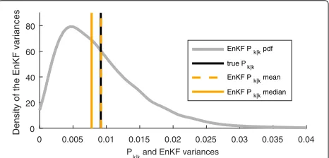
A trajectory of (33) is simulated and a KF is used to compute the optimal variancesPk|k. Because the model is time-invariant, thePk|k quickly converge to a constant value. Fork>3,Pk|k =0.0092 is obtained.
Next, 10,000 Monte Carlo experiments with a sampling-based EnKF withN = 5 are performed. The distribution of obtained P¯k|k fork = 10 is illustrated in Fig. 1. The
0 0.005 0.01 0.015 0.02 0.025 0.03 0.035 0.04
P and EnKF variances 0
20 40 60 80
Density of the EnKF variances
EnKF P pdf
true P
EnKF P mean
EnKF P median
Fig. 1Distribution of EnKF variancesP¯k|kwithk=10 andN=5 ensemble members for 10,000 runs on the same trajectory. Also shown is the mean and median of all outcomes and the desired KF variancePk|k
vertical lines indicate thePk|k of the KF and the median
and mean of theP¯k|koutcomes.
The averageP¯k|k over the Monte Carlo realizations is close to the desiredPk|k. However, there is a large spread among theP¯k|kand the distribution is skewed toward zero
with its median belowPk|k. AlthoughN > n, there is a
tendency to underestimatePk|k.
In order to clarify the reason for this behavior and whether it has to do with the coupling between the EnKF
¯
Kkand the ensemble members, we repeat the experiment
with an EnKF that uses the gain of the stationary KF for allk. The resulting outcomes are illustrated in Fig. 2. Now, the averageP¯k|k is correct. However, the median shows
that there is still more probability mass belowPk|k. The
tendency to underestimatePk|k and the remaining spread
must be due to random sampling errors. For largerN, the effect vanishes, and the median and mean ofP¯k|k appear
similar forN ≥10.
7.2 The particle filter benchmark
In the second example, we show that the EnKF does not converge to the Bayesian filtering solution in nonlin-ear systems as N→ ∞ [31]. A well-known benchmark
0 0.005 0.01 0.015 0.02 0.025 0.03 0.035 0.04
P and EnKF variances 0
20 40 60 80
Density of the EnKF variances
EnKF P pdf
true P
EnKF P mean
EnKF P median
problem from the PF literature [6] is used. The model is specified by
xk+1= xk
2 +25
xk
1+x2k +8 cos(1.2(k+1))+vk,
(34a)
yk=
1 20x
2
k+ek, (34b)
with independent vk ∼ N(0, 10), ek ∼ N(0, 1), and x0∼N(0, 1). Because the model is scalar, the Bayesian fil-tering densitiesp(xk|y1:k) can be computed numerically using point mass filters (PMF) [77]. A sampling based EnKF withN=500 is tested and kernel density estimates are used to obtain approximations ofp(xk|y1:k)from the
ensembles. For comparison, we include a closely related sigma point KF variant that uses Monte Carlo integration with N = 500 samples [5]. The only difference to the EnKF is that this Monte Carlo KF (MCKF) carries out the KF measurement update (5) to propagate a mean and a variance. We illustrate the results as Gaussian densities.
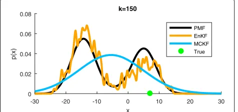
Figure 3 shows the prediction results fork = 150. The PMF reference solution is bimodal with one mode close to the true state. The reason for this lies in the squared
xkin (34b). The EnKF prediction resembles the PMF well
except for the random variations in the kernel density esti-mate. The MCKF cannot represent the multimodality but the Gaussian bell covers the relevant regions.
The filtering results fork=150 are shown in Fig. 4. The PMF reference solution has much narrower peaks after including yk. The EnKF provides a skewed density that
does not resemblep(xk|y1:k)even though the EnKF
pre-diction approximatedp(xk|y1:k−1)well. This is the main take-away result and confirms [31]. Again, the MCKF exhibits a large variance.
Further filtering results for the PMF and EnKF are shown in Fig. 5. It can be seen that the EnKF solutions sometimes resemble the PMF very well but not always. Similar statements can be made for the prediction results.
-30 -20 -10 0 10 20 30
x 0
0.02 0.04 0.06 0.08
p(x)
k=150
PMF EnKF MCKF True
Fig. 3Prediction densitiesp(xk|y1:k−1)by the PMF, EnKF, and MCKF fork=150. The true state is illustrated with agreen dot. The PMF serves as reference solution
-30 -20 -10 0 10 20 30
x 0
0.1 0.2 0.3 0.4
p(x)
k=150
PMF EnKF MCKF True
Fig. 4Filtering densitiesp(xk|y1:k)by PMF, EnKF, and MCKF for k=150. Otherwise similar to Fig. 3
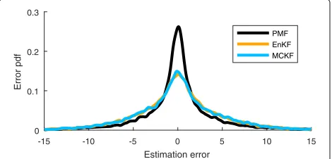
Dots in Fig. 5 illustrate the mean values as state esti-mates. Especially for the PMF, it can be seen that the mean (though optimal in a minimum variance sense [3]) is debatable for multimodal densities. Often, all estimates are quite close. Figure 6 provides the estimation error den-sities obtained from 100 Monte Carlo experiments with 151 time steps each. The PMF mean estimates exhibit a larger peak around 0. The estimation errors for the EnKF and MCKF appear similar. This is surprising because the latter employs a Gaussian approximation at each time step. Both error densities have heavier tails than the PMF density. All estimation errors appear unbiased.
7.3 Batch smoothing using the EnKF
We here show how to use the EnKF as smoothing algo-rithm by estimating batches of states. This allows us to compare its performance for N < n in problems of arbitrary dimension.
-30 -20 -10 0 10 20 30
x 120
121 122 123 124 125
Filtering densities at time k
PMF EnKF True state PMF mean EnKF mean MCKF mean
-15 -10 -5 0 5 10 15 Estimation error
0 0.1 0.2 0.3
Error pdf
PMF EnKF MCKF
Fig. 6Density of the estimation errors obtained from 100 Monte Carlo runs with 151 time steps each
First, we formulate an “augmented state” that comprises an entire trajectory ofL+1 steps,
ξ =xT0 x1T . . . xTL T, (35)
with dimensionn = (L+1)nx. Second, we note that the
measurementsyk, k = 1,. . .,L, have uncorrelated
mea-surement noise and known relations to the components ofξ. For linear systems (1), the predicted mean and covari-ance ofξ can be easily derived, and smoothed estimates of all xk, k = 0,. . .,L, can be obtained by sequentially
processing allykin KF measurement updates forξ. Also, other smoothing variants and the Rauch-Tung-Striebel (RTS) algorithm can be derived from state aug-mentation approaches [3]. Due to its sequential nature, however, the RTS smoother does not provide joint covari-ance matrices ofxkandxk+ifori=0. Except for this and
the higher computational complexity of working withξ, the batch and RTS smoothers are equivalent for (1).
An EnKF approach to batch smoothing mimics the above. A prediction ensemble forξ is obtained by simu-latingN trajectories for random process noise and initial state realizations. This can also be carried out for non-linear models (2). Then, sequential EnKF measurement updates are performed for allyk.
For our experiments, we use a tracking problem with a constant velocity model [67] and position measurements. The low-dimensional state is given by
x=x yx˙ y˙T (36a)
and comprises the Cartesian position [m] and velocity [m/s] of an object. The parameters of (1) are given by
F=
I2 TI2
0 I2
, G= T2
2I2
TI2
, H=I2 0
, (36b)
withT = 1 s. The initial statex0 is Gaussian distributed with
ˆ
x0=0 0 15 −10T, P0=diag(502, 502, 202, 202), (36c)
-1.5 -1 -0.5 0 0.5
Position in km -0.4
-0.2 0 0.2
Position in km
Fig. 7Illustration of a representative trajectory (black), the RTS smoothing solution (cyan), and an initial ensemble (N=50,orange).
Red circlesdepict the measurements. Most ensemble trajectories go beyond the plot area
and the process and measurement noise covariances are
Q=diag(10, 50), R=
2000 1000 1000 1980
. (36d)
Withnx=4 andL=49 we obtainn=200 as dimension
ofξ. The RTS solution is compared to EnKF of ensem-ble sizeN = {10, 20, 50}. Monte Carlo errors are reduced using (21) in the gain computations.
A realization of a true trajectory and its measurements is provided in Fig. 7 together with the RTS estimate and an ensemble ofN=50 trajectories. The latter are the ini-tial ensemble of an EnKF. The ensemble is well gathered around the initial position but fans out wildly.
Figure 8 shows the ensemble after an update withyL
only. The measurement at the end of the trajectory pro-vides an anchor point and quickly reduces the spread of the ensemble. Figure 9 shows the result after processing all measurements in sequential order from first to last. The true trajectory and the RTS estimate are mostly covered well by the ensemble. The EnKF withN=50 appears con-sistent in this respect. Position errors for the RTS and the EnKF are provided in Fig. 10. The EnKF performs slightly worse than the RTS but still gives good results forN=50, without extra inflation or localization.
The next experiment explores the EnKF for N =
10. Figure 11 shows the ensemble after processing all measurements. The ensemble is compactly gathered but
-1.5 -1 -0.5 0 0.5
Position in km -0.4
-0.2 0 0.2
Position in km
-1.5 -1 -0.5 0 0.5 Position in km
-0.4 -0.2 0 0.2
Position in km
Fig. 9The ensemble of Fig. 7 after updating with all measurements in the ordery1,. . .yL. The RTS solution is covered well
does not cover the true trajectory well. The EnKF is overconfident.
A last experiment explores how well an EnKF with
N = 20 captures the uncertainty of the state estimate. Furthermore, we discuss effects of the order in which the measurements are processed. Specifically, we compare the ensemble covariance of the positionsxk to the exact
cov(xk,xi),i,k= 0,. . .,L, obtained by KF updates for the
augmented stateξ.
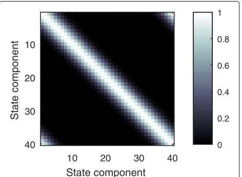
The exact covariance after processing all measurements is shown in Fig. 12. Rowkin the matrix defines the covari-ance function betweenxk and the remainingxpositions.
The banded structure indicates that subsequent positions are more related than, say,x0andxL. Figure 13 shows the
corresponding EnKF covariance after processing the mea-surements from y1 to yL. The off-diagonal elements do
not decay uniformly as in Fig. 12, and spurious positive and negative correlations appear. Furthermore, the cor-rect temporal order of measurements entails an unwanted structure. Laterxk are rated more uncertain according to
the lighter areas in the lower right corner of Fig. 13. A covariance after processing the measurements in random order is shown in Fig. 14. The spurious correlations persist but the diagonal elements appear more homogeneous.
From the above experiments, we conclude that the EnKF can provide good estimates for ensembles with N < n. However, there is a minimum N required to obtain
0 5 10 15 20 25 30 35 40 45
Time step k
20 40 60
Position error
RTS EnKF
Fig. 10Position errors of the RTS (cyan) and the EnKF (N=50,
orange) after updating with all measurements in the ordery1,. . .yL
-1.5 -1 -0.5 0 0.5
Position in km -0.4
-0.2 0 0.2
Position in km
Fig. 11An ensemble withN=10 after updating with all measurements in the ordery1,. . .yL. The smaller ensemble is more condensed and does not cover the RTS solution well
consistent results without further measures such as local-ization or inflation. We have shown adverse effects such as ensembles with too little spread and spurious correlations. As a final note, the alert reader will recognize paral-lels between the above example and ensemble smoothing methods as presented in [17].
7.4 The 40-dimensional Lorenz model
Our final example is a benchmark problem from the EnKF literature. We investigate the 40-dimensional Lorenz-96 model3from [53] that is used in, e.g., [36, 38, 42, 50, 52, 63, 69].
The statexmimics an atmospheric quantity at equally spaced locations along a circle. Its evolution is specified by the nonlinear differential equation
˙
x(j)=x(j+1)−x(j−2)x(j−1)−x(j)+F(j),
(37)
where j = 1,. . ., 40 indexes the components ofx, with the convention that x(0) = x(40) etc. Instead of the commonly used forcing termF(j) = 8, we assume time-dependent Fk(j) ∼ N(8, 1) that are constant for time
0 10 20 30 40
time step k
0
10
20
30
40
time step k
-200 -100 0 100 200 300 400 500
0 10 20 30 40
time step k
0
10
20
30
40
time step k
-200 -100 0 100 200 300 400 500
Fig. 13EnKF (20 members) position covariance matrix cov(xi, xj)after including all measurements in the ordery1,. . .yL
intervalsT=0.05 only and act as process noise. A Runge-Kutta method (RK4) is used to discretize (37) to obtain the nonlinear state difference Eq. (2a) withxk = xk and vk = Fk. The step sizeT corresponds to about 6 h if x
were an atmospheric quantity on a latitude circle of the earth [53]. Although the model (37) is said to be chaotic, the effects are only mild for short integration timesT. In our experiments, all n = 40 states are measured with additive Gaussian noiseek ∼ N(0,I). The initial state is
Gaussian withx0 ∼ N(0,P0), whereP0is drawn from a Wishart distribution with seed matrixInandndegrees of
freedom.
Figure 15 illustrates how the state evolves over sev-eral time steps. There is a tendency for peaks to move “westwards” askincreases.
0 10 20 30 40
time step k
0
10
20
30
40
time step k
-200 -100 0 100 200 300 400 500
Fig. 14EnKF (20 members) position covariance matrix cov(xi, xj)after including all measurements in random order
5 10 15 20 25 30 35 40
State component 30
35 40 45 50 55 60
State at time step k
Fig. 15State evolution for the Lorenz model. Eachhorizontal line
carries a 40-dimensional state vector
We note that there are also alternative approaches for estimatingx, for example, by first linearizing and then dis-cretizing (37). However, we adopt the RK4 discretization of the EnKF literature that yields a state transition that is easy to evaluate but difficult to linearize. Because of this, the EKF [3] cannot be applied easily and we obtain a challenging benchmark problem.
We use sampling-based EnKF to estimate long state sequences ofL = 104time steps. Following [38, 42], the performance is assessed by the error
εk =
1
n(xˆk|k−xk) T(xˆ
k|k−xk), (38)
wherexˆk|kis the ensemble mean. We use the averageεkfor k=100,. . .,L, denoted byε, as quantitative performance¯ measure for different EnKF. Useful EnKF must yieldε <¯ 1, which is the error when simply takingxˆk|k=yk.
First, we compute a reference solution using an EnKF withN =1000. Without any localization or inflationε¯= 0.29 is achieved. Figure 16 shows the sample covariance
¯
Pk|k−1of a prediction ensembleXk|k−1, our best guess of the true covariance. The banded structure reveals that the problem is suitable for localization. Hence, we construct a matrixρfor covariance tapering from a compactly sup-ported correlation function [70] that is also used in [14, 26, 38, 43] and appears to be the standard choice. The chosen ρis a Toeplitz matrix because the components ofxkare at
equidistant locations and shown in Fig. 17.
Next, EnKF with different ensemble sizesN, covariance inflation factorsc, with or without tapering, are compared. The obtained errors ε¯ are summarized in Table 1. For
10 20 30 40
State component
10
20
30
40
State component
-0.1 0 0.1 0.2 0.3 0.4
Fig. 16Prediction covarianceP¯k|k−1fork=30 obtained from an EnKF withN=1000. The banded structure justifies the use of localization
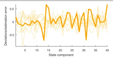
ensemble deviationsXk|k are illustrated. The estimation
error is mostly contained in the intervals spanned by the ensemble; hence, the EnKF is consistent. Tests on EnKF with N = 20 reveal convergence problems, even with inflation the initial estimation error persists. With the help of tapering, however, a competitive error can be achieved. Even further reduction toN = 10 is possible with taper-ing and inflation. The required inflation factorcmust be increased to counteract the lack of ensemble spread. Sim-ilar to Figs. 18 and 19 illustrates the estimation error and deviation ensemble for k = 104, N = 10, c = 1.05, and tapering withρ. Although the obtained error is larger than forN = 40, the ensemble deviations represent the estimation uncertainty well.
A number of lessons have been learned from related experiments. As alternative to theρin Fig. 17, a simpler taper that contains only ones and zeros to enforce the
10 20 30 40
State component
10
20
30
40
State component
0 0.2 0.4 0.6 0.8 1
Fig. 17The employed tapering matrixρ
Table 1Averaged errorsε¯for different EnKF
N c ρ ε¯
1000 1 No 0.29
40 1 No 0.44
40 1.05 No 0.33
40 1 Yes 0.29
40 1.02 Yes 0.28
20 >1 No >1
20 1.01 Yes 0.3
10 1.05 Yes 0.34
banded structure was used. Although thisρ was indefi-nite, a reduction inε¯was achieved without any numerical issues. Hence, the specific structure of ρ appears sec-ondary. The smooth ρ of Fig. 17 remains preferable in terms of ε, though. Sequential processing of the mea-¯ surements did not degrade the performance. Experiments without process noise give the lower errorsε¯ from, e.g., [38, 42].
8 Conclusions
With this paper, we have given a comprehensive and easy to understand introduction to the EnKF for signal pro-cessing researchers. The origin of the EnKF in the KF and its simple implementation have been demonstrated. The unique literature review provides quick access to the most relevant papers in the plethora of geoscientific EnKF pub-lications. Furthermore, we have discussed the challenges related to small ensembles for high-dimensional states,
N < n, and the available solutions such as localization or inflation. Finally, we have tested the EnKF on signal processing and EnKF benchmark problems.
With its scalability and simple implementation, even for nonlinear and non-Gaussian problems, the EnKF stands out as viable candidate for many state estimation prob-lems. Furthermore, localization ideas and advanced con-cepts for estimating covariance matrices and the EnKF
5 10 15 20 25 30 35 40
State component
-1 -0.5 0 0.5 1
Deviations/estimation error
5 10 15 20 25 30 35 40
State component
-0.5 0 0.5
Deviations/estimation error
Fig. 19The estimation errorxk− ¯xk|kfork=104with the deviation ensembleXk|kin the background for an EnKF withN=10, covariance localization, and inflation factorc=1.05
gain from the limited information in the ensembles pro-vide new research directions for the EnKF and high-dimensional filters in general, hopefully with an increased participation from the signal processing community.
Endnotes
1With over 3000 citations between 1994 and 2016.
2We assume that the components can be processed
sequentially.
3Also known as the Lorenz-96, L95, L96, or L40 model.
Acknowledgements
This work was supported by the project Scalable Kalman Filters granted by the Swedish Research Council (VR).
Authors’ contributions
MR wrote the majority of the text and performed the majority of the simulations. GH and CF contributed text to earlier versions of the manuscript and helped with the simulations. GH, CF, and FG commented on and approved the manuscript. FG initiated the research on ensemble Kalman filters. All authors read and approved the final manuscript.
Competing interests
The authors declare that they have no competing interests.
Publisher’s Note
Springer Nature remains neutral with regard to jurisdictional claims in published maps and institutional affiliations.
Received: 28 February 2017 Accepted: 19 July 2017
References
1. E Kalnay,Atmospheric modeling, data assimilation and predictability. (Cambridge University Press, New York, 2002)
2. RE Kalman, A new approach to linear filtering and prediction problems. J. Basic Eng.82(1), 35–45 (1960)
3. BD Anderson, JB Moore,Optimal filtering. (Prentice Hall, Englewood Cliffs, 1979)
4. S Julier, J Uhlmann, H Durrant-Whyte, inProceedings of the American Control Conference 1995vol.3. A new approach for filtering nonlinear systems (IEEE, Seattle, 1995), pp. 1628–1632
5. M Roth, G Hendeby, F Gustafsson, Nonlinear Kalman filters explained: a tutorial on moment computations and sigma point methods. J Adv. Inf. Fusion.11(1), 47–70 (2016)
6. NJ Gordon, DJ Salmond, AF Smith, Novel approach to
nonlinear/non-Gaussian Bayesian state estimation. Radar Signal Process. IEE Proc. F.140(2), 107–113 (1993)
7. F Gustafsson, Particle filter theory and practice with positioning applications. IEEE Aerosp. Electron. Syst. Mag.25(7), 53–82 (2010) 8. G Evensen, Sequential data assimilation with a nonlinear
quasi-geostrophic model using Monte Carlo methods to forecast error statistics. J. Geophys. Res. Oceans.99(C5), 3–10162 (1014)
9. G Burgers, JP van Leeuwen, G Evensen, Analysis scheme in the ensemble Kalman filter. Mon. Weather Rev.126(6), 1719–1724 (1998)
10. H Durrant-Whyte, T Bailey, Simultaneous localization and mapping: Part I. IEEE Robot. Autom. Mag.13(2), 99–110 (2006)
11. M Baum, UD Hanebeck, Extended object tracking with random hypersurface models. IEEE Trans. Aerosp. Electron. Syst.50(1), 149–159 (2014)
12. N Wahlström, E Özkan, Extended target tracking using Gaussian processes. IEEE Trans. Signal Proc.63(16), 4165–4178 (2015)
13. PL Houtekamer, HL Mitchell, Data assimilation using an ensemble Kalman filter technique. Mon. Weather Rev.126(3), 796–811 (1998)
14. PL Houtekamer, HL Mitchell, A sequential ensemble Kalman filter for atmospheric data assimilation. Mon. Weather Rev.129(1), 123–137 (2001) 15. AH Jazwinski,Stochastic processes and filtering theory. (Academic Press, New
York, 1970)
16. G Evensen, The ensemble Kalman filter: theoretical formulation and practical implementation. Ocean Dyn.53(4), 343–367 (2003)
17. G Evensen,Data assimilation: the ensemble Kalman filter, 2nd ed. (Springer, Dordrecht, New York, 2009)
18. TM Hamill, inPredictability of Weather and Climate. Ensemble-based atmospheric data assimilation (Cambridge University Press, Cambridge, 2006)
19. PL Houtekamer, HL Mitchell, Ensemble Kalman filtering. Q. J. R. Meteorol. Soc.131(613), 3269–3289 (2005)
20. JS Whitaker, TM Hamill, X Wei, Y Song, Z Toth, Ensemble data assimilation with the NCEP global forecast system. Mon. Weather Rev.136(2), 463–482 (2008)
21. GP Compo, JS Whitaker, PD Sardeshmukh, N Matsui, RJ Allan, X Yin, BE Gleason, RS Vose, G Rutledge, P Bessemoulin,
S Brönnimann, M Brunet, RI Crouthamel, AN Grant, PY Groisman, PD Jones, MC Kruk, AC Kruger, GJ Marshall, M Maugeri, HY Mok, O Nordli, TF Ross, RM Trigo, XL Wang, SD Woodruff, SJ Worley, The twentieth century reanalysis project. Q. J. R. Meteorol. Soc.137(654), 1–28 (2011)
22. S Lakshmivarahan, D Stensrud, Ensemble Kalman filter. IEEE Control. Syst. 29(3), 34–46 (2009)
23. J Anderson, Ensemble Kalman filters for large geophysical applications. IEEE Control. Syst.29(3), 66–82 (2009)
24. G Evensen, The ensemble Kalman filter for combined state and parameter estimation. IEEE Control. Syst.29(3), 83–104 (2009) 25. J Mandel, J Beezley, J Coen, M Kim, Data assimilation for wildland fires.
IEEE Control. Syst.29(3), 47–65 (2009)
26. R Furrer, T Bengtsson, Estimation of high-dimensional prior and posterior covariance matrices in Kalman filter variants. J. Multivar. Anal.98(2), 227–255 (2007)
27. M Butala, J Yun, Y Chen, R Frazin, F Kamalabadi, in15th IEEE International Conference on Image Processing. Asymptotic convergence of the ensemble Kalman filter (IEEE, San Diego, 2008), pp. 825–828 28. J Mandel, L Cobb, JD Beezley, On the convergence of the ensemble
Kalman filter. Appl. Math.56(6), 533–541 (2011)
29. M Frei,Ensemble Kalman Filtering and Generalizations(Dissertation, ETH, Zürich, 2013). nr. 21266
30. M Katzfuss, JR Stroud, CK Wikle, Understanding the ensemble Kalman filter. Am. Stat.70(4), 350–357 (2016)
31. F Le Gland, V Monbet, V Tran, inThe Oxford Handbook of Nonlinear Filtering, ed. by D Crisan, B Rozovskii. Large sample asymptotics for the ensemble Kalman filter (Oxford University Press, Oxford, 2011), pp. 598–634 32. M Butala, R Frazin, Y Chen, F Kamalabadi, Tomographic imaging of
dynamic objects with the ensemble Kalman filter. IEEE Trans. Image Process.18(7), 1573–1587 (2009)
33. J Dunik, O Straka, M Simandl, E Blasch, Random-point-based filters: analysis and comparison in target tracking. IEEE Trans. Aerosp. Electron. Syst.51(2), 1403–1421 (2015)