Efficient Implementation of Nested-Loop
Multimedia Algorithms
Surin Kittitornkun
Department of Electrical and Computer Engineering, University of Wisconsin, Madison, WI 53706, USA Email: [email protected]
Yu Hen Hu
Department of Electrical and Computer Engineering, University of Wisconsin, Madison, WI 53706, USA Email: [email protected]
Received 22 June 2001 and in revised form 22 August 2001
A novel dependence graph representation called themultiple-order dependence graphfor nested-loop formulated multimedia sig-nal processing algorithms is proposed. It allows a concise representation of an entire family of dependence graphs. This powerful representation facilitates the development of innovative implementation approach for nested-loop formulated multimedia algo-rithms such as motion estimation, matrix-matrix product, 2D linear transform, and others. In particular, algebraic linear mapping (assignment and scheduling) methodology can be applied to implement such algorithms on an array of simple-processing ele-ments. The feasibility of this new approach is demonstrated in three major target architectures: application-specific integrated circuit (ASIC), field programmable gate array (FPGA), and a programmable clustered VLIW processor.
Keywords and phrases:dependence graph, systolic array, multiple-order, FPGA, VLIW.
1. INTRODUCTION
Many data-intensive multimedia algorithms such as motion estimation, 2D DCT/IDCT, matrix multiplication, and others consist of mainly deep nested-loops with relatively simple-loop body. They have been painstakingly implemented man-ually as hardwired ASICs (application specific integrated cir-cuits) [1, 2] in order to meet the extremely high throughput rate demand of video signal processing algorithms. In view of the repetitive nature of the nested-loop algorithm formu-lation, the most effective strategy to speed up computation is to realize such an algorithm using an array of processing elements (PEs) to facilitate parallel processing.
In 1967, Karp et al. [3] introduced the notion of uni-form recurrence equationas a powerful abstraction to describe nested-loop algorithm formulations. Lamport [4] considered the parallel execution of Do loops and proposed to use the al-gebraic construct of ahyperplanein the iteration index space to characterize the iterations that can be executed simulta-neously. In 1982, Kung [5] and Leiserson [6] used the term systolic arrayto describe the pipelined execution of nested-loop formulated algorithms in a regular-structured, locally connected array of identical PEs. It has been argued that a sys-tolic array structure is amenable for very large scale integra-tion circuit (VLSI) implementaintegra-tion as it exploits maximum
parallelism while requiring only local communication among processors. In the 1980s, Kung [7] and others [8, 9] have de-veloped systematic design methodologies for systolic arrays. These methods facilitate algebraic mapping of the iteration indices of a nested-loop onto a systolic array with a linear task assignment and a linear schedule implementation.
With the rapidly increasing demands for real-time multi-media signal processing applications, it becomes ever impor-tant to pursue efficient implementation of data intensive mul-timedia processing algorithms. As pointed out earlier, many of them are suitable for parallel implementation using sys-tolic array of PEs. One notable example is the numerous 1D and 2D array structures of block-based motion estimation algorithm [10, 11, 12, 13, 14].
bandwidth. In a conventional dependence graph, every execu-tion (data delivery) order must be explicitly specified. When there are multiple-choices of loop execution (data delivery) orders, one must select a specific execution order (data deliv-ery) using heuristic. These premature commitments of par-ticular orders often prevent an optimal implementation to be found.
In this paper, we propose a novel dependence graph repre-sentation, calledmultiple-order dependence graph(MODG). In a MODG, all the permissible execution (data delivery) or-ders will be represented explicitly in a concise format. As such, a single MODG representation can represent many of equiv-alent DGs. Since each of these equivequiv-alent DGs may lead to a locally optimal design, searching all of them combined is more likely to yield a globally optimal design.
As noted above, systolic array architecture style so far has been applied mainly for hardwired ASIC modules. With the advancement of deep submicron system-on-chip (SOC) manufacturing technology, it becomes clear that the cost of interconnect in terms of propagation delay, power consump-tion, and chip real estate has increased so much compared to that of logics. Furthermore, the speed gap between logic and dynamic memory gets widened.
As such, the architecture style of a regular array of pro-cessing elements with mostly local interconnects can be found in several different architecture styles. For example, modern field programmable gate array (FPGA) architectures such as the Xilinx Vertex II and the Altera APEX II are composed of a regular array of LUTs (look-up tables) and static RAM blocks as local storage. Even modern programmable digital signal processors also adopted aclustered VLIW(very long instruc-tion word) architecture where the collecinstruc-tion of funcinstruc-tional units and a local register file within a cluster can be regarded as a powerful processing elements (PEs). These clusters can be programmed as a multiprocessor system to achieve parallel processing [16, 17].
In the remaining of this paper, we will first introduce basic definitions and the novel representation of MODG in Section 2. Then the design methodology based on MODG will be presented in Section 3. Next, we illustrate the advan-tages of MODG using three design examples: a hardwired ASIC implementation of block-based motion estimation, an FPGA implementation of matrix-matrix multiplication, and the implementation of separable 2D transform on a 4-cluster VLIW processor in Sections 4, 5, and 6, respectively. Lastly, Section 7 concludes this paper.
2. MULTIPLE-ORDER DEPENDENCE GRAPH
In this section, a novel representation of nested-loop, called multiple-(execution) order dependence graphas well as the ba-sic definitions of dependence analysis will be introduced. The motivation for a multiple-order dependence graph represen-tation will then be presented prior to its formal definition.
2.1. Nested-loop formulated algorithms
Many digital signal processing, image and video processing algorithms can be formulated compactly with a nested-loop
formulation. Consider the following example of a matrix-matrix multiplication algorithm.
Example1. Matrix-matrix multiplicationC=A×B
ci,j= K
k=1
ai,kbk,j, (1)
where A = [ai,j],B = [bi,j], andC = [ci,j]are matrices
of appropriate dimensions. The corresponding nested-loop algorithm formulation can be expressed as:
Listing1. Matrix-matrix multiplication multiple times
Doi=1to3
Doj=1to3 c[i, j]=0
Dok=1to3
c[i, j]=c[i, j]+a[i, k]×b[k, j]
EndDok
EndDoj
EndDoi
where i,j, andk are loop indices. Together, they form an (iteration)index spacewhere each point(i, j, k)corresponds to a single execution of theloop body.
In general, letimbe themth level loop index of loop-nest,
andi = (i1, i2, . . . , in)t ∈ Zbe ann-dimensional column
index vector of an n-level nested Do-loop where Z is the space of integer numbers andatdenotes the transposition of
a. Hence, then-Dindex spaceJncan be expressed as:
Jn=i=(i1, i2, . . . , in)t|i1, i2, . . . , in∈Z. (2)
In this example, the loop body consists of a single recur-rence equation
c[i, j]=c[i, j]+a[i, k]×b[k, j], (3)
wherea[i, k]andb[k, j]areinput variablesand their values are needed to execute this loop,c[i, j]’s areoutput variables whose values will be computed by executing the loop-nest.
In Listing 1, the innermostk-loop is used to realize the summation ofKproduct termsa[i, k]×b[k, j],1≤k≤K. While c[i, j]is the final result, it is also used to store in-termediate results atkth iteration. In other words, the same memory address designated toc[i, j]is assigned to new val-ues multiple-times during the execution of the algorithm. In asingle-assignmentformulation [7], we introduce a set of new intermediate variables to store the intermediate results. As such, every variable will be assigned to a new value at most once during the execution of the algorithm.
In this example, the input variablea[i, k] will be used in each of the j loops, and b[k, j]will be used in each of the iloops. In particular,a[i, k] will be made available to iterations with indices{(i, j, k)t; 1≤j≤N}, andb[k, j]will
be made available to iteration indices{(i, j, k)t; 1≤i≤M}
different iterations are executed at different processors, these input variables must be propagated or broadcast to different processors to facilitate the computation. This routine of input variables can be represented using intermediate variables to ensure that the single-assignment constraint is satisfied.
With the introduction of the intermediate variables, every variable associated with a particular iteration will have the full set of indices. For example, the matrix-matrix multiplication loop body can now be rewritten as follows.
Listing2. Single-assignment matrix-matrix multiplication
Doi=1toM
In the listing above,a3andb3are thetransmittal variables
ofaandb, respectively, andc3is thecomputation variableof c. We may also define an inter-iterationdependence vector as the set of index differences between the output of each iteration (on the left-hand side of each equation) and the input (on the right-hand side of the recurrence equations). Therefore, the dependence vector of variablea3,b3, andc3
are da3 = (0,1,0)t,db3 = (1,0,0)
t, andd
c3 = (0,0,1)t,
respectively.
A loop-nest is called a set of uniform recurrence equa-tions(URE) [3] if its loop bounds are not functions of any output variables in the loop body and its dependence vec-tors are independent of the loop index i. In other words, a
URE’s loop bounds are known constants before the execution of the algorithm. Almost all the data intensive nested-loop formulated multimedia algorithms are uniform recurrence equations. In general, a URE algorithm satisfying the single-assignment constraint can be described in a representation as shown in Figure 1 wherelmandumareim’s lower and upper
bounds andm=1,2, . . . , n.
Three types of statement are included in the innermost loop body: the Input/propagation statement, the Computa-tion/initialization statement, and theOutput statement. Each type of statement corresponds to a particular type of the vari-ables.
•Transmittal variable.An input variablevjis first
assign-ed to the transmittal variablevjn[i]at iteration indicesi∈II vj, and then propagated along apropagationdependence vector
Figure1:n-level nested Do-loop algorithm.
Compared to Listing 2, we havea3[i]andb3[i]as
trans-mittal variables wherei=(i, j, k)t. The initialization spaces
ofa3andb3areIIa3 = {(i, j, k)t|1≤i≤M,1≤k≤K, j= 0}andII
b3 = {(i, j, k)
t | 1 ≤ j ≤ N,1 ≤ k ≤ K, i = 0},
respectively.
•Computation variable.The computation variablevkn[i]
will be initialized to some constants at index set (iterations)
i ∈IN
vk, and then will be assigned to output values at other iterationsi∈IC
vk according to the recurrence functionFvk. Use Listing 2 as an example, we haveIN
c = {(i, j,0)t|1≤ i ≤ M,1 ≤ j ≤ N}andIC
c = {(i, j, k)t | 1≤ i ≤ M,1≤ j ≤ N,1 ≤ k ≤ K}. The operatorFvk is the summation operation.
• Output variable. These are results that will be stored back to memories outside the processor array. Their values will be assigned at a set of output index pointsIO
vk. From Listing 2,c[i, j]is the output variable and IO
c = {(i, j, k)t|k=K}. The indexing function of output variable cisGc(i, j, k)=(i, j)ifk=K.
Based on the URE algorithm formulation, a set of data dependence vectorscan be identified.
•Propagationdependence vector:dv
j. In Example 1,
da=(0,1,0)t, db=(1,0,0)t. (4)
•Computationdependence vector:dv
k. Likewise,
dc=(0,1,0)t. (5)
+ ×
c
a
a
a
a
a
a
a
a
a
b b b
b
b b
b b
b
c c
c
c
c
(a)
11= 0 11
11
12
12
13
23
33
13
23
33 32
31 33
32 31
21
21 22
32 31
13
23 22
b
a
c
a
b
c
(b)
Figure2:3×3matrix-matrix multiplication in a 3D dependence graph (a) and its node (loop body)(b).
The dependence vectors constrain the execution order that must be followed to ensure correctness of the algorithm. However, we note that in this example, alternate execution orders are possible:
(a) Since the operation of summation is invariant to any permutation of its operands, we may obtain the same result by reversing the direction of the dependence vector(0,0,1)t
to(0,0,−1)t. This leads to a different execution order
c[i, j, k]=c[i, j, k+1]+a[i, j, k]×b[i, j, k]. (6)
(b) Since the transmittal variables remain unchanged throughout the execution, the actual transmission direction will not be critical. Hence, instead of using current depen-dence vectors(1,0,0)t,(0,1,0)t, one may also use alternate
dependence vectors(−1,0,0)t,(0,−1,0)t.
Clearly, with the set of alternate dependence vectors, dif-ferent, yet functionally equivalent dependence graph may be constructed. Motivated by this observation, we set out to pro-pose a powerful way to represent a dependence graph and all those dependence graphs with alternative execution orders in a unified manner. We call itmultiple-(execution) order depen-dence graph(MODG).
2.2. Ann-dimensional multiple-order dependence graph (n-D MODG)
The dependence graph [7] or the iteration space dependence graph [18] is a graphical representation of data dependen-cies among loop iterations of a nested Do-loop. A directed
dependence graph consists of a set of nodes (vertices) and a set of edges. Each node corresponds to a loop index,i∈Jn, or
the innermost loop body regardless of its complexity. Each di-rectional edge represents either a propagation or a computa-tion dependence vector. It can be observed from Figure 2 that the 3-level nested Do-loop results in a 3D dependence graph. In contrast, we define an MODG as a set of MODG nodes where each node is associated with a number of information fields including edges as dependence vectors as follows.
Definition 2 (n-dimensional multiple-order dependence graph,Kn). Ann-D MODG,Kn, is a set of MODG nodes.
Each node,kn∈Kn, is a collection of the following fields of
information,n-D index, multiple-order dependence vectors set, input data set, output data set, and terminal flag set.
Eachn-D MODG node,kn ∈Kn, containing a tuple-of
information fields can be written as
kn
i, DV, IV, OV, FV
, (7)
where V is a set of variables. Similar to C++ object ori-ented programming language, we use “.” to access a partic-ular field. For example, kn.i denotes an n-D index field, kn.i = (i1, i2, . . . , in)t ∈ Jn, kn.IV is a set of input data,
wherekn.IV = {kn.Iv | ∀v ∈V}.Likewise,kn.OV is a set
of output data,kn.OV = {kn.Ov | ∀v ∈ V}. Next, a set
kn.FV = {kn.Fv | ∀v ∈V}whereFv ∈ {0,1}andFv =1
denotes the true logic value. Finally,kn.DV is a set of
depen-dence vectors associated with variable setV,
kn.DV =kn.Dv| ∀v∈V, (8)
wherekn.Dvdenotes a set of all feasible dependence vectors
of variable v.kn.Dv can be obtained depending upon the
following categories of variables.
2.2.1 Transmittal variable
In traditional systolic design methodology, each instance of input variablev[ g]is reused and propagated according to a single dependence vectordvas shown in Figure 1, that is,
kn.Dv=dv, ∀kn.i∈IPv∪IIv. (9)
This dependence vector is determined during the algorithm formulation and restricted to an adjacent or neighboring index. Hence, the propagation along a particular direction based on heuristic is imposed such that the dependence graph becomes localized. Once it is input inside the processor array, it is called thetransmittalvariable instead.
Actually, each instance v[ g] of the variable v can be reused several times during the course of execution. Order-ing should not be imposed as long as it is delivered correctly. To represent all the possible dependence vectors among all reusing MODG nodes, we define abroadcast index setas a set ofn-D indices associated with each instance of variable
v[ g],
Igv=kn.i| Hvkn.i=g, ∀kn∈Kn, (10)
where
Hv(i):i−→g, ∃i∈IPv∪IIv. (11)
The indexing function Hv is similar to Gv(i). Therefore,
at any index point, each variable is associated with a set of multiple-order dependence vectors
kn.Dv=i1−kn.i|kn.i≠i1,∀i1∈Igv (12)
including the localized dependence vectordv.
2.2.2 Computation variable
In a nested Do-loop algorithm, the computation variablevis an output of a particular recurrence functionFv. This
func-tion can be as simple as add, multiply, minimum, maximum, and the like. If these operators follow both commutative and associative laws such that
Fv(a, b)= Fv(b, a), FvFv(a, b), c= Fva,Fv(b, c)
= Fvb,Fv(a, c),
(13)
respectively, they are calledmultiple-orderoperators. Other-wise, functions or operators that do not follow both laws are
consideredin-order. Traditionally, each instance of compu-tation variablev is computed and propagated along a local dependence vectordv, that is,
kn.Dv=dv, ∀kn.i∈INv∪ICv, (14)
as if it were an in-order operation.
Given a multiple-order operation, the instancev[ g]can be computed in many different orders of execution. Ordering should be relaxed provided that it is semantically correct and its numerical condition is satisfied. To represent all the possi-ble dependence vectors among all computing MODG nodes, we definea multiple-order index setas a set of MODG nodes of a variablev[ g]to be
Igv=kn.i| Hvkn.i=g, ∀kn∈Kn, (15)
where
Hv(i):i−→g, ∃i∈INv∪ICv. (16)
Therefore, a set of multiple-order dependence vectors of vari-ablevcan be obtained as
kn.Dv=i1−kn.i|kn.i≠i1, ∀i1∈I g
v. (17)
Back to the matrix product example, we can identify the indexing functions G as Ga(i, j, k) = (i, k) if j = 0,
Gb(i, j, k)=(k, j)ifi=0, andGc(i, j, k)=(i, j)ifk=K.
The indexing function H of both input variables,aandb
areHa(i, j, k)=(i, k)andHb(i, j, k)=(k, j), respectively. Since the summation follows both associative and commu-tative laws, it is a multiple-order operation and its indexing functionHc(i, j, k)=(i, j).
2.3. Summary
We call the dependence graph with multiple-order depen-dence vectors for both propagation and multiple-order oper-ator a multiple-order dependence graph (MODG). Although MODG contains cycles due to those multiple-order depen-dence vectors, no self loops are introduced. MODG is still computable because it is formulated based on the computable dependence graph [7]. After the mapping is applied, a few of dependence vectors will become feasible and the final one will be selected appropriately. The mapping methodology will be introduced in the following section.
3. MAPPING METHODOLOGY OF MODG
Due to the regular structure of n-D MODG, the task of scheduling and assignment of each index (loop body) to execute on a number of processing elements (PEs) at a certain clock cycle becomes an algebraic projection. This projection is called systolic or space-timemapping. As a consequence, the index spaceJnis mapped (both assigned and scheduled)
3.1. 1D space-time mapping
We propose the 1D space-time mapping ofn-D MODG to a 1D array of PEs. The advantages of 1D array are three folds. First, the final 1D array can be adjusted to fit the chip area easily. Second, the input/output port is already on the array boundary. Third, the array is easy to rearrange to a 2D array. The 1D mapping matrix is defined below.
Definition 3 (1D space-time mapping matrix,T1). The 1D
space-time mapping matrixT1consists of a scheduling vector
sand an allocation vectorPas,
T1=
array representation to accommodate the mapping. In a big picture, the mapping process can be visualized as shown in Figure 3.
Definition4 (1D processing element array,K1). A 1D PE array
is a set of nodes or PEs in which each node is resulting from a projection of a number of n-D MODG nodes. Each PE encapsulates the PE number and a clock schedule of feasible delay-edge pairs, input/output data, and terminal flags.
In other words, each PE is a tuple of (J1, t(i), RV, EV, rV, eV, IV, OV, FV). Input, output, and terminal sets are
as-signed to a PE and ordered according to the synchronous schedulek1.t(i). Each PE is equivalent to a set ofn-D MODG
The clock schedule associated with eachk1∈K1is obtained
from
the space-time mapping of the multiple-order dependence vectors of an MODG node, such that
In addition, the terminal flag set at this cycle τ becomes
k1.FV[τ] = {k1.Fv[τ] | ∀v ∈ V} where k1.Fv[τ] = kn.Fv. Finally, the final edge-delay pair,k1.ev[τ]−k1.rv[τ], k1.ev[τ] ∈ k1.Ev[τ], k1.rv[τ] ∈ k1.Rv[τ], are chosen
appropriately subject to the design objectives (performance) and design constraints (cost) in the next two subsections.
Although this 1D mapping matrixT1was originally
pro-posed by Lee and Kedem [19], ours is different from theirs in the following aspects:
•There is no restriction on the ratio of delay and edge length.
•Input and output ports are not necessary at either end of the array.
•Ours can be applied to several different target architec-tures such as ASIC, FPGA and clustered VLIW which will be illustrated later.
3.2. Mapping objective functions: performance
The 1D PE array can be evaluated based on the following per-formance characteristics. As objective functions, the number of cycles, the number of PEs, and the utilization are analogous to the execution time, the area, and the efficiency in hard-ware, respectively. Besides, physical input/output pins and memory bandwidth are of increased importance as the speed gap between logic and memory especially dynamic RAM gets wider. Additionally, these objective functions can be used to constrain the optimization as well.
3.2.1 Number of cycles(Ncycle)
For ASIC implementation, the total parallel execution time,
ttotal, can be computed by
ttotal=tcycle×Ncycle, (23)
where tcycle is the PE’s longest critical propagation delay,
which depends on the PE architecture and the implemen-tation technology, andNcycleis the number of clock cycles
[7] given by
In other words, it is the number of cuts by the equitempo-ral hyperplane [4] perpendicular to the scheduling vectors. AlthoughNcycleseems to depend on the scheduling vectors
only, the question on how many PEs are utilized and how the data are delivered to the right PE still remains.
3.2.2 Number of PEs(NPE)
In the 1D or linear array mapping, the number of PEs,NPE
can be expressed as
NPE=PEmax−PEmin+1. (25)
In other words,NPEis the number of distinct projections of
the index spaceJnon the vectorP.
3.2.3 Utilization(U )
k1,1 t(i)E I F Ov1
Ov2 Ov0
Iv1 Iv2 I
Ov1 Ov2 Ov0
k1,0 Iv1
Iv2 Iv0
Ov1
Ov2 Ov0
kn,m
Iv1 Iv2 Iv0
Ov1
Ov2 Ov0
kn,2m−1 Iv1
Iv2 Iv0
Ov1 Ov2 Ov0
Iv1 Iv2 Iv0
Ov1 Ov2 Ov0 T1
1D space-time mapping
n-D MODG
1D time schedule 1D space assignment
0 1 2 3 kn,0
kn,m−1 Iv1
Iv2 Iv0
VRV VOV V v0
. . .
Figure3: Space-time mapping ofn-D multiple order dependence graph to a 1D processor array.
by
Umax=
maxτk1|τ∈k1.t(i) NPE
, (26)
where |a|denotes the cardinality or size of set a. On the other hand, the average utilization is the ratio of the number of MODG nodes and theNcycle−NPEproduct,
Uavg=
Kn NPE×Ncycle
. (27)
3.2.4 Number of input/output ports(#IO)
Due to limited number of physical I/O pins of a given target architecture, it is important to minimize the number of I/O ports. Based on our formulation, the set of PEs performing I/O of either input or output variablevat cycleτis
IOv[τ]=
k1|k1.Fv[τ]=1, τ∈k1.t(i), ∀k1∈K1
.
(28) Therefore, the number of variablev’s I/O ports is given by
#IOv=max
τ IOv[τ], (29)
where|IOv[τ]|denotes the size ofIOv[τ].
3.2.5 Memory bandwidth
The memory bandwidth associated with variable v,
Bv, is the number of input/output instances via a
particular input/output port per unit time. In this case, the unit time is a clock cycle. From (28),Bvis equivalent to the
to-tal number of input/output occurrences averaged overNcycle,
Bv=
τ∈k1.t(i),∀k1∈K1IOv[τ]
Ncycle . (30)
3.3. Design constraints
3.3.1 Mapping conflict
Due to insufficient rank ofT1, a mapping conflict occurs when
two MODG nodes are assigned to the same PE and scheduled at the same cycle, that is, T1p = T1q,p ≠ q,p, q ∈ Jn.
Unlike [19, 20], nocommunication conflictis introduced by our method. In order to efficiently detect the conflicts, a 2D integer arrayAof sizeNPE×Ncycleis used,
Conflict=No←→iff A[T1q] ≤1, ∀q∈Jn, (31)
where
A[T1q] =
0 initialization, AT1q +1 otherwise.
(32)
Each array element A[T1q] is increased by one if the
previous value is zero from the initialization phase. Oth-erwise, the computation conflict is detected. The worst-case time complexity of this method is O(Nn)whereN= max{ui−li+1, i=1,2, . . . , n}while that of [19] isO(N2n).
3.3.2 Propagation constraint
Despite the fact that a systolic array can achieve high com-putation throughput, one of the reasons that it has not been successful is partly due to its high demand of memory band-width. As a result, every input variable should be traced and reused as many times as possible to eliminate redundant memory fetches. Thus, we can eventually save the bandwidth and the number of I/O ports. Hence, the input port should be determined after the mapping process rather than from a predetermined terminal flag assigned by a human designer. The input port is assigned to ak1PE where the first instance
of data appears and propagated to the next instance. Permis-sible edge-delay pairs are obtained by eliminating edges that point backward in the time domain.
The mapping process starts by initializing the terminal vectors kn.Fv = 0,∀kn ∈ Kn. After space-time mapping,
the terminal flag will be true at the first appearance in the broadcast index setIgvof each input instancev[ g]. Thus, the
terminal flag is assigned by
k1.Fv[τ]=
1, τ=mink1.t(i) 0, τ >mink1.t(i) ∀
kn.i∈I g v. (33)
3.3.3 Multiple-order operation constraint
Likewise, given an output variablevafter mapping, the ter-minal flag will be true at the last appearance in the multiple-order index set of each instancev[ g],Igvin (15). Thus, the
terminal flag is assigned by
k1.Fv[τ]=
1, τ=maxk1.t(i)
0, τ <maxk1.t(i) ∀ kn.i∈I
g v. (34)
3.3.4 Causality constraint
The purpose of this causality constraint is to prevent consum-ing intermediate data before it is fully produced. For every
instance of intermediate producer variable vp[ f ] and
instance of consumer variablevc[ g], the following inequality
must be satisfied.
maxstp| ∀p∈Ifvp
<minstq| ∀q∈Igvc
. (35)
3.4. Heuristic search
Due to the exponential growth in both area and time com-plexity of MODG, its mapping methodology must be lim-ited to some heuristic search. To be competitive in the mar-ket, some strategies are necessary to cut the design time and cost. From the definition of T1 in (18), its elements
are limited to si ∈ {0,±1,±li ±1,±ui±1} and pi ∈ {0,±1,±li±1,±ui±1}. As a matter of fact that the search
is independent to one another, a number of different iter-ations can be distributed in a network of workstation [21] and compared to the performance evaluations at the end. Finally, the problem size should be scaled down to reduce the computational complexity.
3.5. Summary
In summary, the mapping can be cast as an optimization problem with the objective functions in Section 3.2 subject to the design constraints in Section 3.3 with some search strate-gies in Section 3.4. Furthermore, the search of T1 must be
subject to the architecture mapping constraints of hardwired ASIC, FPGA, and clustered VLIW processor in the subsequent sections, respectively.
4. HARDWIRED ASIC MAPPING
It has been widely accepted that the full search block match-ing (FSBM) motion estimation is one of the most time-consuming task for digital video encoding. Several hardwired ASICs have been manufactured including the STi3220 mo-tion estimamo-tion processor [1]. As a major step towards saving memory bandwidth, Yeo and Hu [13] proposed the formu-lation of a six-level nested Do-loop algorithm to represent a single-frame, multiple-block motion estimation. A typical video frame consists ofNh×Nvblocks of pixels whereNhis
the number of blocks in each row andNvis the number of
rows of block in each frame. A motion vector,(m, n)of an
N×N block of pixels, which yields the minimum mean-absolute distortion (MAD) between current block and the
(2p+1)2blocks in the search area, can be obtained by
MV=argmin MAD(m, n)−(p, p), 0≤m, n≤2p,
(36) wherepis thesearch rangein number of pixels and usually less than or equal to block sizeN. The corresponding MAD of a vector(m, n)is obtained by
MAD(m, n)= N−1
i=0 N−1
j=0
x(i, j)−y(i+m−p, j+n−p),
Do-loop MAD-based FSBM algorithm is shown in Figure 4 whereDminis theminimum distortionmeasured using MAD.
It can be noticed thatMAD(m, n)andminare of multiple-order operators. In addition, it has been observed in [14] that there are many possible data propagation patterns. Therefore, the proposed MODG is applicable.
Dov=0toNv−1
Doh=0toNh−1
MV (h, v)=(0,0);
Dmin(h, v)= ∞;
Dom=0to2p
Don=0to2p
MAD(m, n)=0;
Doi=0toN−1
Doj=0toN−1
MAD(m, n)=MAD(m, n)+
x(hN+i, vN+j)
−y(hN+i+m−p, vN+j+n−p);
EndDoj,i
ifDmin(h, v) >MAD(m, n)
Dmin(h, v)=MAD(m, n); MV (h, v)=(m−p, n−p);
endif EndDon,m,h,v
Figure4: Six-level nested Do-loop FSBM motion estimation algo-rithm.
4.1. Result
Due to the limited presentation space, we can scale the prob-lem size down toNv=3,Nh=3,N=4, andp=N/2=2.
As indicated earlier in Section 3, T1 must be searched to
obtain the final 1D array that satisfies numerous constraints. The heuristic search is limited to the surrounding regions to the previous result from [14, 15]. Our objective is to equalize the bandwidth of current frame pixelxand previous frame pixelywhile minimizingNcycle.
The optimal solution is
T1=
N2 NhN2 2p+1 2 N 1 0 0 2p+1 1 0 0
. (38)
The permissible edges-delay pair of each PE, k1.ev[τ]− k1.rv[τ],v ∈ {x, y, Dmin}, was chosen in such a way to
minimize the total number of registers (delay elements). Depicted in Figure 5, the 2D array is obtained semi-automatically where the indicates the input ports to the array. On the other hand, the schedules of current frame pixelx(i, j), previous frame pixely(i, j)atτ =35,36, and 37 are listed in Figure 6(a), (b), and (c), respectively. Each
x(i, j)propagates from left PE to right PE every two cycles in parallel and to the consecutive row every five cycles only in the first column. The propagation ofDminis of the similar
pattern while the final result is the minimum one among all rows. The previous frame pixelsy(i, j)propagate downward every cycle and to the right PE in the first row only. Although the schedules show that two y(i, j) pixels are needed per cycle, every y(i, j) is fetched once and reused throughout the entire execution.
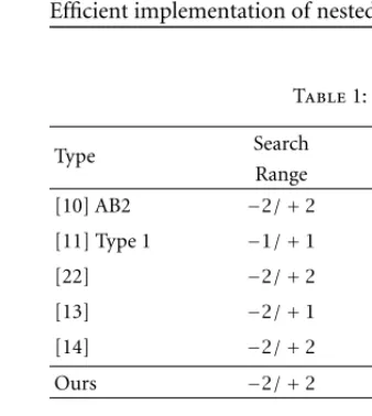
4.2. Discussions
Table 1 quantitatively compares different aspects among 2D arrays in terms of search range,NPE, throughput (cycles per
block), memory bandwidth ratio By/Bx, and fan-out. We
were able to achieve unity By/Bx bandwidth ratio. It can
be noticed that oursBy/Bx ratio is superior to others with
a few more registers to compensate with the huge demand ofy’s memory bandwidth. The less bandwidth demand, the less pressure on the on-and off-chip memory becomes. The array can eliminate redundant memory fetches thus preserve memory (I/O) transactions as well as power consumption at the same time.
We definefan-out as the total number of loads (sinks) whose source has more than two loads. It essentially repre-sents the undesirable broadcasting mechanism. Greater fan-out implies bigger effective capacitanceCeffwhich the
prop-agation delay as well as the power consumption according to the very well-known equation,
Power∝CeffVsup2 fCLK, (39)
where Vsup andfCLK are the supply voltage and operating
clock frequency, respectively.
It can be observed at this point that the MODG and its mapping methodology can reduce redundant memory fetches of previous frame pixels by at least50%while achiev-ing frame-level pipelinachiev-ing [14], and no broadcast. The bot-tom line is that this 2D array isnot achievablefrom the tra-ditional mapping methodology [7]. That is because every variable instance must propagate/compute in only one direc-tion by enforcing a uniform edge-delay pair. The MODG can represent the motion estimation loop-nest as if it were rep-resented in human thinking which results in a more flexible array structure and more efficient implementation.
5. FPGA ARCHITECTURE MAPPING
PE PE
architecture is the SRAM-based FPGAs such as those of Xilinx Virtex family.
5.1. Programmable-length shift register
It is a magnificent feature of the look-up table (LUT) of an SRAM-based FPGA and can be exploited by our design methodology to propagate input data that are unknown at design time. Each LUT can be programmed as 1-bit of length
N≤16. Hence, an 8-bitN-cycle delay consumes only 8 LUTs ifN≤16rather than8Nflip/flops or equivalently8NLUTs in FPGA because one flip/flop is provided per LUT [24]. For an input variablevat PEk1∈K1, the final edge-delay pair
at cycleτ∈k1.t(i)is subject to the following equations.
k1.rv[τ] >0, k1.ev[τ]≠0,
k1.ev[τ]k1.rv[τ]=mink1.RV[τ]k1.Ev[τ].
(40)
5.2. Distributed ROM/RAM
Besides working as the 4-bit input/1-bit output Boolean func-tion generator, an LUT can be utilized as a single- or dual-port ROM/RAM. According to [24], two LUTs in the same slice can
be configured as a single-port32×1-bit ROM/RAM or a dual-port16×1-bit ROM/RAM . Unlike hardwired ASIC design, FPGA can be reconfigured with any initialization values em-bedded in the configuration bit stream. ROM and RAM are suitable for input and output variables, respectively. This is due to the fact that RAM can be updated while ROM cannot. However, the control mechanism is a little more complex.
For a constant and known input variablevat PEk1∈K1,
the delay and edge sets at cycleτ∈k1.t(i)are subject to the
following equations to utilize the distributed ROM:
k1.Rv[τ]=
mN|N >0, m≠0, m∈Z, k1.Ev[τ]= {0}.
(41)
The constraints are the same for an output variablevto use distributed RAM.
5.3. Three-state buffer
Table1: Performance comparison for 2D FSBM ME arrays,N=4,p=N/2=2.
Type Search NPE Throughput Registers By/Bx Fan-Out
Range (Cycles/Block) (bytes)
[10] AB2 −2/+2 16 40 94 10 0
[11] Type 1 −1/+1 16 40 180 2 100
[22] −2/+2 16 65 94 4 0
[13] −2/+1 16 16 64 2 16
[14] −2/+2 25 16 152 2 8
Ours −2/+2 25 16 164 1 0
9,4 9,3 8,6 8,5 7,8 9,3 9,2 8,5 8,4 7,7 9,2 8,5 8,4 7,7 7,6 9,1 8,4 8,3 7,6 7,5 8,4 8,3 7,6 7,5 6,8
9,5 9,4 9,3 8,6 8,5 9,4 9,3 8,6 8,5 7,8 9,3 9,2 8,5 8,4 7,7 9,2 8,5 8,4 7,7 7,6 9,1 8,4 8,3 7,6 7,5 11,6 11,4 10,6 10,4 9,6
10,5 10,3 9,5 9,3 8,5 9,4 8,6 8,4 7,6 7,4 8,3 7,5 7,3 6,5 6,3 6,6 6,4 5,6 5,4 4,6
12,3 11,5 11,3 10,5 10,3 10,6 10,4 9,6 9,4 8,6 9,5 9,3 8,5 8,3 7,5 8,4 7,6 7,4 6,6 6,4 7,3 6,5 6,3 5,5 5,3
12,4 11,6 11,4 10,6 10,4 11,3 11,5 10,3 9,5 9,3 9,6 9,4 8,6 8,4 7,6 8,5 8,3 7,5 7,3 6,5 7,4 6,6 6,4 5,6 5,4
9,6 9,5 9,4 8,7 8,6 9,5 9,4 9,3 8,6 8,5 9,4 9,3 8,6 8,5 7,8 9,3 9,2 8,5 8,4 7,7 9,2 8,5 8,4 7,7 7,6 (a)
x(i,j) y(i,j)
(b)
(c)
Figure6: Schedule of full search block matching motion estimation: (a) at cycleτ =35, (b)τ=36, and (c)τ =37(Nh=3,Nv=3, N=4,p=N/2=2).
strategy consumes virtually zero LUT provided that built-in three-state buffers are inherently available from the occupied logic LUTs. A bus-based design for an output variable vis subject to the following constraints:
#IOv[τ]=1, ∀τ∈k1.t(i), ∀k1∈K1
#IOv>1.
(42)
5.4. Other constructs
Algorithms that involve inner dot products such as FIR filters can exploit the LUTs to store filter coefficients and fast-carry adders using distributed arithmetic [25]. In modern the 10-million-gate FPGA architecture like Xilinx Virtex II, a number of highly optimized 18-bit×18-bit multipliers are provided and distributed throughout the chip [26].
5.5. Example: matrix-matrix multiplication
Matrix-vector and -matrix multiplications are the fundamen-tal operation of 1D orthogonal transform, 2D/3D graphics, and many others. A number of 1D processor arrays have been proposed in [19, 20, 27, 28]. However, their results suffer from low processor utilization due to propagation constraints of unknown input data. Normally, the coefficient matrix is known beforehand. We can exploit this fact using MODG to FPGA architecture mapping.
We letx,c, andybe theN×Ninput, coefficients, and output matrices, respectively, where
y=cx. (43)
The algorithm can be formulated as 3-level nested Do-loop as shown earlier. Our goal is to minimizeNPEandNcyclewhile
achieving 100% maximum utilization, single-port pipelined input datax, stored coefficientsc, and single-port output data
y. In a bounded solution space, the heuristic search pruned out more than half of the invalid solutions according to the mapping constraint in (31). Then, only the valid solutions were evaluated subject to the following constraints: the prop-agation inputxin (40), the distributed ROM for coefficients
cin (41), and the bus-based output constraint in (42). This transformation matrixT1is one of the solutions
T1=
−1 −4 1 1 0 0
. (44)
From (24) and (25) we achieveNPE=4andNcycle=19from
the PE array and its clock schedule as shown in Figures 7 and 8, respectively. The propagation of inputxis pipelined along the array to multiply with the stored coefficientscin each PE. The outputyis accumulated every cycle and placed on the bus everyNcycles. The output bus interface exploits abundant three-state buffers of FPGA. The schedule is equivalent to cutting the original 3D MODG of a matrix-matrix product into 2D slices, tiling each slice of MODG to a 2D MODG, and projecting the tiled 2D MODG to a 1D PE array.
PE x PE PE PE
En En
y
En En
ROM
addr c
ROM
addr
ROM
addr
ROM
addr
x x x
c c c
0 1 2 3
0 1 2 3
Figure7: Architecture of pipelined busN×Nmatrix multiplicationN=4.
0 1 2 3 0 -- -- -- 41 1 -- -- 31 42 2 -- 21 32 43 3 11 22 33 44 4 12 23 34 41 5 13 24 31 42 6 14 21 32 43 7 11 22 33 44 8 12 23 34 41 9 13 24 31 42 10 14 21 32 43 11 11 22 33 44 12 12 23 34 41 13 13 24 31 42 14 14 21 32 43 15 11 22 33 44 16 12 23 34 17 13 24 18 14
0 1 2 3 0 -- -- -- 14 1 -- -- 14 24 2 -- 14 24 34 3 14 24 34 44 4 24 34 44 13 5 34 44 13 23 6 44 13 23 33 7 13 23 33 43 8 23 33 43 12 9 33 43 12 22 10 43 12 22 32 11 12 22 32 42 12 22 32 42 11 13 32 42 11 21 14 42 11 21 31 15 11 21 31 41 16 21 31 41 17 31 41 18 41
--(a) (b)
NPE NPE
Ncycle
Figure8: Schedule of pipelined busN×Nmatrix multiplication N=4: (a) coefficientc[i, j]and (b) inputx[i, j].
the fewer resources it utilizes. Ours is even better since its target architecture is the FPGA. Due to the known coeffi-cient matrixc, we saveM =8pins whereM isc’s andx’s bit precision and y is of 3M-bit precision. The utilization figures,Umax andUavg, are of importance when the power
supply is limited. Unlike ours, other PE arrays spend most of the time propagating data. Finally, latency is more con-cerned as the delay from applying input to getting the first output increases which results in less hardware utilization. Each single-port N-entryM-bit ROM consumesN/16M
LUTs [24] where x denotes the smallest integer greater than or equal to x. The LUT consumption ratio of [27] to ours is over 3.85 with the multiplier built from LUTs. The ra-tio would increase up to 5.25 if the Virtex II architecture were assumed because each built-in multiplier does not consume any LUT [26].
Table2: Matrix-matrix product,N = 4,M =8is the precision (bits) (Virtex FPGA is assumed).
Performance [27] [19] [20] [28] Ours
PE Array 1D 1D 1D 1D 1D
Ncycle 31 19 19 19 19
NPE 8 10 10 10 4
Umax 50% 60% 70% 60% 100%
Uavg 25.8% 33.7% 33.7% 33.7% 84.2%
Latency(cycles) 8 18 18 25 4
#IO(pins) 6M 5M 5M 5M 4M
LUTs/PE 216 168 144 136 112
LUTs Ratio 3.85 3.75 3.21 3.04 1.00
Table3: Number of LUTs/PE,N=4,M=8is the precision (bits) (Virtex FPGA is assumed).
Performance [27] [19] [20] [28] Ours
(24+16)-b Adder 24 24 24 24 24
(8-bit×8=16)-b Multiplier 48 48 48 48 48
24-by’s Registers 72 72 48 24 24
8-bc’s Registers 56 8 16 24 8
8-bx’s Registers 16 16 8 16 8
Total 216 168 144 136 112
Table 3 enumerates the number of LUTs estimated for datapath of each PE. The Xilinx core generator system pro-vides not only the netlists of those components in PE datap-ath, that is, bit-parallel adder, multiplier, and others but also the accurate estimation of LUTs consumption. This allows the designer to predict the complexity of each PE in advance. On the other hand, the control circuitry of each PE was diffi-cult to estimate because it is mechanism dependent and varies from architecture to architecture. Note that the mapping can be applied to matrix products of any size.
6. CLUSTERED VLIW MAPPING
After the extensive study of multimedia workload [16] espe-cially video encoding/decoding, it has been analyzed that a video signal processor should be equipped with a large num-ber of ALUs (arithmetic and logic units), shifters, multipli-ers, and multiported register file to gain the available data parallelism. Current examples of clustered VLIW processor are the TI’s C6X Velociti and the analog device’s TigerSharc families. The Princeton video signal processor [17, 29, 30] has been recently proposed and targeted at 1 GHz operating clock frequency. In order to achieve the goal, the so-called clusteredVLIW has been adopted with up to eight homoge-neous clusters of functional units. Some time-critical video signal processing algorithms involve deep nested Do-loop such as 2D DCT/IDCT (discrete cosine transform/inverse discrete cosine transform), block-based motion estimation, and others.
However, the current instruction scheduling of clustered VLIW is limited to basic block level [31] and tries to per-form both partitioning and instruction scheduling to all clus-ters [32]. Particularly multimedia workload, inter-procedure analysis, and loop transformation are needed to discover coarse-grain parallelism that is not visible at basic block level [17]. Hence, there is not enough instruction-level parallelism (ILP) to fully utilize the available hardware parallelism.
As a coarse-grain loop pipelining methodology, the MODG and its space-time mapping can be applied to fully exploit loop-level parallelism. We assume the clustered VLIW architecture just like the Princeton video signal processor with predicate execution capability currently adopted by the Intel IA64 architecture. The algorithm to its architecture mapping is subject to the following constraints. However, these con-straints can be used as objective functions as well.
6.1. Number of clusters(C)
SinceNPEis a function of problem size, it can be greater than
the number of clustersC after the mapping. The solutions are constrained such that the number of PEs is an integer multiple- of the number of clusters.
NPE=mC, (45)
where m > 0,m ∈ Z. Therefore,m PEs will be mapped to the same cluster. This is beneficial to instruction sched-uler because basic block will be expanded so that intracluster parallelism can be exploited.
6.2. Intercluster communication channels
The number of intercluster transactions should be minimized to avoid being communication bottleneck. The links can be implemented as crossbar switches [30] or busses [31]. In each PE or cluster k1, the number of occurrences of
nonzero-length edge and nonnegative delay pair of variable v can be expressed as{τ| ∃k1.Ev[τ]i>0,∃k1.Rv[τ]i≥0}where k1.Ev[τ]i and k1.Rv[τ]i are theith element of k1.Ev[τ]
andk1.Rv[τ], respectively. Hence, its cardinality yields the
number of intercluster transactions of PEk1∈K1.
6.3. Local register file size
If the loop is unrolled according to the obtainable solution, the basic block will be enlarged and instruction scheduler will be able to exploit ILP more. However, the number of registers needed may grow. Since each cluster has its own local register file, register allocation can be performed independently. To aid the register allocation using graph coloring such as the one proposed by Chaitin et al. [33], live range of each variable instance can be obtained to formulate register interference graph. For each processor number k1.J1 the LiveRange of
variable instancev[ g]can be written as
LiveRangegv
=maxst( p−q) | ∀p, ∀q∈Ivg, k1.J1=Ptp=Ptq.
(46)
6.4. Local memory space
The number of variable v’s instances in the PE of pro-cessor number k1.J1 is the cardinality of the following set, {g|Pt(k
n.i)=k1.J1,∃kn.i ∈Igv}. The total space of local
memory required in each cluster is the summation over all variables,∀v∈V. The size of local memory should be large enough to hold all necessary variable instances. For example, local memory of 2 Kbytes per cluster is projected by [16].
6.5. Example: 2D separable transformation
The 2D DCT/IDCT is a common 2D separable linear trans-form in image and video processing. Its matrix-matrix prod-uct is formulated as
X=c(cx)t, (47)
wherec,x, andXare theN×Ntransform coefficient, input and output matrices, respectively. We can rewrite it in a two-pass matrix-matrix multiplication
y=cx, Y=yt, X=cY . (48)
Its single loop-nest algorithm was derived in the appendix for more details. It can be noticed that the innermost loop body is invariant. Therefore, loop collapsing [18] was applied. Eventually, the single-assignment loop and its dependence graph can be illustrated in Figures 9 and 10, respectively. As a result, we could formulate its MODG. The mapping is constrained to the following conditions. First, since practical 2D DCT/IDCT are of N×N elements where N = 8, the mapping is constrained toNPE = C = N = 4in this case.
Second, one input port per input variable,candx. Finally, intercluster transaction should be kept as low as possible. One of the solutions is thisT1,
T1=
−1 −8 1
−1 0 0
. (49)
The assignments and schedules ofx,Y, andcare illustrated in Figure 11. The c[m, n]-x[m, n] pair or the c[m, n]
passes, respectively. The iterations are assigned to clusters 0–3 and skewed/ordered relative to one another to pipeline fetch-ing data from data cache. The overall schedule shows that no intercluster transactions are required. The following is a simple-pseudo assembly code for matrix-matrix product of
y=cx.
According to the loop schedule in Figure 11, the assembly code above is replicated in all four clusters to form a bigger loop body. They are pipelined/skewed by one cycle as shown in Figure 12. We assume that each cluster has one memory load/store unit that takes one cycle latency if data cache hits. Although the first load may stall the following instructions for a certain number of clock cycles, the subsequent loads will take only one cycle due to cache hit. This corresponds to the constraint of having single input port forcandx. The four loop bodies are almost identical and can be scheduled with any existing instruction scheduling algorithm.
Unlike software pipelining that schedules instructions from adjacent loop iterations to the available functional units in any cluster [31], our scheme is different in such a way that each cluster is assigned to execute instructions solely belonging to an independent loop body. In addition, soft-ware pipelining using modulo scheduling [34] yields each result every initiation interval to increase throughput rate which can be limited by the available ILP. Ours instead en-hances the throughput by a larger factor of the number of clustersCexecuting in parallel. Furthermore, the subsequent independent iterations can be executed in parallel if the loop is unfolded and more functional units such as multiple-ALUs and multipliers are available.
7. CONCLUSION
Multimedia signal processing is subject to real-time con-straint, for example, audio/video coding/decoding, 2D/3D
Dom=1toN
Figure9: Single-assignment of two-dimensional separable trans-form algorithm.
graphics. To meet such high throughput demand, either specific integrated circuit (ASIC) or application-specific instruction set processor (ASIP) is often utilized. ASIC can be of the form hardwired ASIC or programmable hardware like FPGA. On the other hand, clustered VLIW architecture is adopted as the main architecture of ASIP to exploit static instruction level parallelism due to predictable behavior of multimedia algorithms.
As a matter of fact that most of multimedia algorithms are characterized as data-intensive and data-parallel algo-rithms. Furthermore, a huge portion of total execution time is consumed by elementary operations such as motion esti-mation, matrix multiplication, 1D/2D linear transform, and others that can be described as nested-loop with simple-innermost loop body. The novel multiple-order dependence graph (MODG) is proposed to represent all possible exe-cution and data delivery orders. Along with its architecture mapping methodology, it is targeted as a computer aided de-sign tool.
c11
c21
c 31
c 12
c22
c 32
c 13
c 23
c 33
x11 x12 x
13
x21
x22 x23
x
32 x33
x31
y33 y
32 y
31
y23
y13
X 11
X 12
X13
X21
X 22
X23
X 31
X32
X33
c
11 c
12 c13
c21
c 22
c 23
c32 c33 c
31 Y33 Y
23 Y
13
Y 32
Y31 m
n
k
Figure10: Dependence graph of two-dimensional transformation,Y=(cx)t,X=cY,N=3.
Firstly, the best-ever 2D systolic motion estimation array was obtained in hardwired architecture. It outperforms others by demanding the least memory bandwidth with mostly local interconnects, small amount of fan-out, and reasonable num-ber of registers. Secondly, we were able to obtain systolic array
-- -- -- 11
Figure11: Schedule of 2D separable transformation: (a) inputx[i, j], (b) intermediate dataY [i, j], and (c) coefficientsc[i, j].
Cluster 0 Cluster 1 Cluster 2 Cluster 3
ldi r12,0
ldi r12,0 ldi r11,0
ldi r12,0 ldi r11,1 ldi r10,0
ldi r12,0 ldi r11,2 ldi r10,0 ldi r3,0
ldi r11,3 ldi r10,0 ldi r3,0 ldi r10,0
ldi r10,0 ldi r3,0 · · · ld r0,c[r12,r10]
Figure 12: Instruction scheduling of cluster-parallel pipelined matrix-matrix product,C=4.
to exploit both cluster level and instruction level parallelism. The methodology acts like a coarse-grain loop pipelining scheduler to parallel available clusters while minimizing intercluster communication.
Although the time and area complexities of the MODG grow exponentially, it is the only concise representation that expresses parallelism explicitly. Moreover, its 1D array target and design constraints as well as heuristic search strategy can counterbalance for its complexity on a modern network of workstations.
APPENDIX
SINGLE-PASS SEPARABLE 2D TRANSFORMATION
Dom=1toN
Don=1toN
Doi=1toN
Dok=1toN
y[i, j]=y[i, j]+c[i, k]×x[k, j]
EndDok
EndDoj
EndDoi X[m, n]=0
Dop=1toN Y [p, n]=y[n, p]
X[m, n]=X[m, n]+c[m, p]×Y [p, n]
EndDop
EndDon
EndDom
After loop collapsing [18], the nested Do-loop above be-comes
Dom=1toN
Don=1toN y[m, n]=0
Dok=1toN
y[m, n]=y[m, n]+c[m, k]×x[k, n]
EndDok X[m, n]=0
Dop=1toN Y [p, n]=y[n, p]
X[m, n]=X[m, n]+c[m, p]×Y [p, n]
EndDop
EndDon
EndDom
REFERENCES
[1] S. Microelectronics, “Sti3220 motion estimation processor,” Jan. 1994.
[2] T. Xanthopoulos and A. P. Chandrakasan, “A low-power dct core using adaptive bitwidth and arithmetic activity exploiting signal correlations and quantization,”IEEE J. Solid-State Circ., vol. 35, no. 5, pp. 740–750, 2000.
[3] R. M. Karp, R. E. Miller, and S. Winograd, “The organization of computations for uniform recurrence equations,” J. ACM, vol. 14, no. 3, pp. 563–590, 1967.
[4] L. Lamport, “The parallel execution of do loops,” Commun. ACM, vol. 17, no. 2, pp. 83–93, 1974.
[5] H. T. Kung, “Why systolic architectures?,”IEEE Comput., vol. 15, no. 1, pp. 37–46, 1982.
[6] C. E. Leiserson,Area-Efficient VLSI Computation, MIT Press, Cambridge, Massachusetts, 1983.
[7] S. Y. Kung, VLSI Array Processors, Prentice Hall, Englewood Cliffs, NJ, 1988.
[8] S. K. Rao and T. Kailath, “Regular iterative algorithms and their implementation on processor arrays,”Proc. IEEE, vol. 76, no. 4, pp. 259–282, 1988.
[9] D. I. Moldovan, Parallel Processing: From Applications to Sys-tems, Morgan Kaufmann, San Mateo, CA, 1993.
[10] T. Komarek and P. Pirsch, “Array architectures for block match-ing algorithms,” IEEE Trans. Circ. Syst., vol. 36, no. 10, pp. 1301–1308, 1989.
[11] L. D. Vos and M. Stegherr, “Parameterizable vlsi architectures for the full-search block-matching algorithm,” IEEE Trans. Circ. Syst., vol. 36, no. 10, pp. 1309–1316, 1989.
[12] K.-M. Yang, M.-T. Sun, and L. Wu, “Vlsi designs for block-matching algorithms,” IEEE Trans. Circ. Syst., vol. 36, no. 10, pp. 1317–1325, 1989.
[13] H. Yeo and Y. H. Hu, “A novel modular systolic array architec-ture for full-search block matching motion estimation,”IEEE Trans. Circuit Syst. Video Technol., vol. 5, no. 5, pp. 407–416, 1995.
[14] S. Kittitornkun and Y. H. Hu, “Frame-level pipelined motion estimation array processor,” IEEE Trans. Circuit Syst. Video Technol., vol. 11, no. 2, pp. 248–251, 2001.
[15] S. Kittitornkun and Y. H. Hu, “Reconfigurable processor array synthesis,” inInt. Conf. Parallel and Distributed Computing, Applications, and Technologies, 2001.
[16] J. Fritts, W. Wolf, and B. Liu, “Understanding multimedia application characteristics for designing programmable media processors,” vol. 3655, pp. 2–13. The International Society for Optical Engineering, 1998.
[17] Z. Wu and W. Wolf, “Design study of shared memory in vliw video signal processor,” inProc. Int. Conf. Parallel Architectures and Compilation Techniques, pp. 52–59. 1998.
[18] M. J. Wolfe, High Performance Compilers for Parallel Comput-ing, Addison-Wesley, Redwood City, CA, 1996.
[19] P. Z. Lee and Z. M. Kedem, “Synthesizing linear array algo-rithms from nested for loop algoalgo-rithms,”IEEE Trans. Comput., vol. 37, no. 12, pp. 1578–1598, 1988.
[20] W. Shang and J. A. B. Fortes, “Time optimal linear schedules for algorithms with uniform dependencies,”IEEE Trans. Comput., vol. 40, no. 6, pp. 723–742, 1991.
[21] Condor high throughput computing, http://www.cs.wisc.edu/ condor/.
[22] C. H. Hsieh and T. P. Lin, “Vlsi architecture for block-matching motion estimation algorithm,”IEEE Trans. Circuit Syst. Video Technol., vol. 2, no. 2, pp. 169–175, 1992.
[23] D. R. Martinez, T. J. Moeller, and K. Teitelbaum, “Application of reconfigurable computing to a high performance front-end radar signal processor,” J. VLSI Signal Processing, vol. 28, no. 1–2, pp. 65–83, 2001.
[24] Xilinx, “Virtex 2.5v field programmable gate arrays,” May 2000. [25] R. D. Turney, C. Dick, D. B. Parlour, and J. Hwang, Modeling
and implementation of dsp fpga solutions, Xilinx.
[26] Xilinx, “Virtex-ii 1.5v field programmable gate arrays,” Jan. 2000.
[27] V. K. P. Kumar and Y.-C. Tsai, “Synthesizing optimal family of linear systolic arrays for matrix computations,” inProc. Int. Conf. Systolic Arrays, pp. 51–60. 1988.
[28] K. G. Ganapathy and B. Wah, “Optimal design of lower di-mensional processor arrays for uniform recurrences,” inInt. Conf. Application Specific Array Processors, pp. 636–648. 1992. [29] S. Dutta, K. J. O’Connor, W. Wolf, and A. Wolfe, “A design
study of a 0.25-µm video signal processor,”IEEE Trans. Circuit Syst. Video Technol., vol. 8, no. 4, pp. 501–519, 1998.
[30] W. Wolf, “Alternative architectures for video signal processor,” inProc. IEEE CS Workshop VLSI, pp. 5–8. 2000.
[31] J. Sanchez and A. Gonzalez, “Modulo scheduling for a fully-distributed clustered vliw architecture,” in Proc. 33rd ann. IEEE/ACM Int. Symp. Microarchitecture, pp. 124–133. 2000. [32] R. Leupers, “Instruction scheduling for clustered vliw dsps,”
inProc. Int. Conf. Parallel Architectures and Compilation Tech-niques, pp. 291–300. 2000.
[33] G. J. Chaitin, M. A. Auslander, A. K. Chandra, J. Cocke, M. E. Hopkins, and P. W. Markstein, “Understanding multimedia application characteristics for designing programmable media processors,”J. Comput. Lang., vol. 3655, pp. 2–13, 1981. [34] B. R. Rau, “Iterative modulo scheduling: An algorithm for
Surin Kittitornkun received his B. Eng (2nd Honor) from King Mongkut’s Insti-tute of Technology Ladkrabang (KMITL), Bangkok, Thailand in 1991. He received M. Eng and Telecom Finland Prize for academic excellence from Asian Institute of Technol-ogy (AIT), Bangkok, Thailand in 1995. He is currently a Ph.D. Candidate at Depart-ment of Electrical and Computer Engineer-ing, University of Wisconsin, Madison. His
research interests include VLSI architecture for digital signal/image processing, and FPGA/reconfigurable computing. He was a sum-mer intern with Broadband Wireless System Department, Motorola, Inc., Schaumberg, IL in 1998.
Yu Hen Hu received a BSEE degree from National Taiwan University, Taipei, Taiwan, ROC in 1976. He received MSEE and Ph.D. degrees in Electrical Engineering from Uni-versity of Southern California, Los Ange-les, California in 1980 and 1982, respec-tively. From 1983 to 1987, he was an assis-tant professor of the Electrical Engineering Department of Southern Methodist Univer-sity, Dallas, Texas. He joined the Department