R E S E A R C H
Open Access
Impacts of frequency increment errors on
frequency diverse array beampattern
Kuandong Gao
*, Hui Chen
†, Huaizong Shao, Jingye Cai and Wen-Qin Wang
†Abstract
Different from conventional phased array, which provides only angle-dependent beampattern, frequency diverse array (FDA) employs a small frequency increment across the antenna elements and thus results in a range angle-dependent beampattern. However, due to imperfect electronic devices, it is difficult to ensure accurate frequency increments, and consequently, the array performance will be degraded by unavoidable frequency increment errors. In this paper, we investigate the impacts of frequency increment errors on FDA beampattern. We derive the beampattern errors caused by deterministic frequency increment errors. For stochastic frequency increment errors, the corresponding upper and lower bounds of FDA beampattern error are derived. They are verified by numerical results. Furthermore, the statistical characteristics of FDA beampattern with random frequency
increment errors, which obey Gaussian distribution and uniform distribution, are also investigated.
Keywords: Frequency diverse array (FDA); Frequency increment errors; Beampattern error; FDA beampattern; FDA radar
1 Introduction
Beampattern is widely used to assess the performance of phased arrays [1]. However, a limitation of phased array is that the beam steering is fixed at one angle for all the ranges [2]. Recently, a flexible array called frequency diverse array (FDA) has been proposed [3-5]. Different from phased array, a small frequency increment, as com-pared to the carrier frequency, is applied across the array elements [6]. This small frequency increment results in a range angle-dependent beampattern [7,8]. Several inves-tigations have been carried on FDA radars. The time and angle periodicity of FDA beampattern was analyzed in [9]. A linear FDA was proposed in [10] for forward-looking radar ground moving target indication. The multipath characteristics of FDA radar over a ground plane were investigated and compared with phased array in [11]. FDA radar full-wave simulation and implementation with linear frequency-modulated continuous waveform were presented in [12,13]. In [14], we have investigated the FDA
*Correspondence: [email protected]
†Equal contributors
School of Communication and Information Engineering, University of Electronic Science and Technology of China, 2008, Road XiYuan, Chengdu, 611731 Sichuan, China
Cramér-Rao lower bounds for estimating direction, range, and velocity. More recent work about the applications of FDA in MIMO radars can be found in [15-19].
Perfect frequency increments are often assumed in existing literatures [20]. However, in an actual array system, there will have imperfect errors including ele-ment position errors, mutual coupling, phase errors, and frequency increment errors [21-24]. Some results have been reported about the impacts of element position error, mutual coupling and phase error on beampattern, and direction-of-arrival (DOA) estimation performances. Since FDA beampattern has similar properties with con-ventional phased array for the impacts of element position errors, mutual coupling, and phase errors, this paper con-siders only the impacts of frequency increment errors on FDA beampattern. Since FDA beampattern is dependent on the angle and range, it has a potential for target local-ization , which is different from traditional time-of-arrival (TOA) and angle-of-arrival (AOA)-based localization [25-28]. The contributions can be summarized as follows. (i) More tighter bounds of FDA beampattern deviation are derived. (ii) Statistical analysis of FDA beampattern in terms of expectation value, variance, and probability density function (PDF) are provided.
The rest of this paper is organized as follows. Section 2 formulates the data models of FDA radar without and with frequency increment errors, respectively. Section 3 analyzes the impacts of deterministic frequency incre-ment errors on FDA beampattern. Thereafter, the impacts of random frequency increment errors are investigated in Section 4. Finally, simulation results are provided in Section 5, and conclusions are drawn in Section 6.
2 FDA beampattern without frequency increment
errors
Suppose an N-element uniform linear FDA with inter-element spacing denoted as d. The radiated frequency from thenth element is as follows:
fn=f0+nf,n=0, 1, 2,. . .,N−1 (1)
wheref0andf are the carrier frequency and frequency increment, respectively. Taking the first element as the reference for the array, under far-field condition, one might express the direct wave component of the electric field emitted from the FDA at the observation point(θ,r)
as [17]:
where N is the number of FDA elements,an represents the complex excitation coefficient for the nth element, ςn(θ|wn)stands for the far-field vector radiation pattern for thenth element at rangerand angular frequencywn= 2πfn,c0is the light speed,dn is the element position of thenth element reference relative to the first element, and
t is the time parameter. In accordance with the far-field
assumption,ejwn
t−r+dnsinθ c0
/rcorresponds to the delayed carrier with free space loss.
To interpret the effect of frequency diversity within the scope of an array factor, we should factor the vector ele-ment pattern out of Equation 2. This can indeed be done under certain conditions. Assuming all elements in the FDA are identical, we can eliminate the frequency depen-dence in the element factor. Since r dn, we have:
ςn(θ|wn)≈ς(θ|w0). (3)
wherew0is the carrier angular frequency. So Equation 2 can be rewritten as:
A(θ,r,t)=ς(θ|w0)
Further simplification becomes possible by considering particular FDA arrangements that are simple to handle and yet able to provide valuable insight. A uniform lin-ear FDA utilizing discrete, linlin-ear frequency increments is such a practical configuration, and it is examined in this
section as a special case. By definition, the elements are excited with uniform amplitude, but they are allowed to have a phase progression across the array. These specifica-tions translate to the following expressions fordnandan:
dn=nd and an=e−jnφa (5)
where φa stands for the phase progression. Submitting Equations 1 and 5 into Equation 4 yields:
A(θ,r,t)=ς (θ|w0)
be rewritten as:
A(θ,r,t)= ς¯
Sincendsinθ r, Equation 7 can be reformulated as:
A(θ,r,t)≈ ς¯ hermitian transpose operator, respectively. For simplicity,
¯
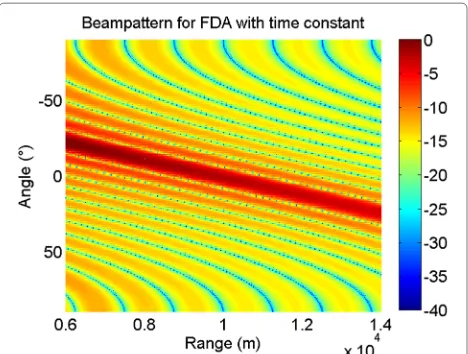
ς = 1 is assumed in the following discussions. Figure 1 shows the ideal linear uniform FDA beampattern with
t=1/f.
2.1 FDA beampattern with frequency increment errors
Suppose the frequency increment errors being ρ = [ 0 ρ1 . . . ρN−1], Equation 8 can be rewritten as:
A(θ,r)= w
Hv˜(θ,r,t)
Figure 1Ideal two-dimension FDA beampattern withN=16,
Then Equation 11 can be reformulated as:
˜
denotes a diagonal matrix withv(r,t)being its diagonal elements. For small frequency increment errors, Taylor series expansion aboutCis performed as follows:
C(r,t)=I+C+(r,t). (14)
According to Equation 13, it can be known that:
C+(r,t)=diag FDA radar, andO(ρ)represents for the high order terms about ρ, which can be ignored for Equation 15. Using Equation 15, we can rewrite the beampattern (13) as:
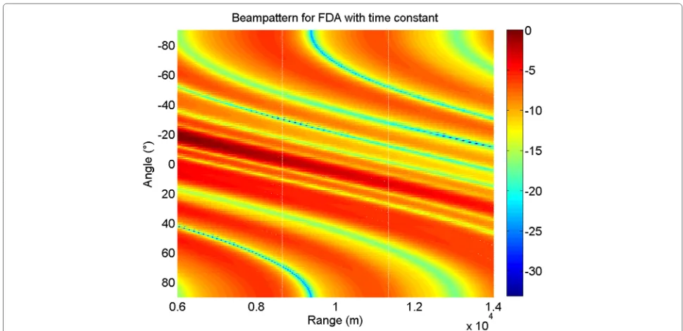
˜ pattern deviation. Figure 2 shows the FDA beampattern with frequency increment errors. The array parameters are the same as that for Figure 1. Due to the frequency increment errors, the FDA beampattern sidelobes are dif-ferent from Figure 1. Stronger sidelobe peaks will make the FDA energy scattering and consequently degrade the array performance.
3 Impacts of deterministic frequency increment
errors
Firstly, we consider uniform frequency increment errors, i.e., ρ = [0ρ1. . . ρN−1] = [0ρ . . . ρ]. In this case, Equation 13 can be rewritten as:
Figure 2Two-dimension FDA beampattern with frequency increment errorρnandρn∼N(0,ρ2)withρ=500.
wherek =ejπN
t(f+ρ)−cr0(f+ρ)−f0dsinc0θ
andw= 1N×1. Equation 17 arrives the maximum value when:
f
t+ ρ
ft
−f
c0
r+ ρ
fr
−
f0
dsinθ
c0
=2m
m=0, 1, 2,. . ..
(18)
If no frequency increment error exists, the FDA main-lobe will pass the location0◦, c0
f
att = 1f. However, when there are frequency increment errors, the location
0◦, c0 f
may be not at the beampattern maximum point. According to Equation 18, the corresponding range error is as follows:
r= ρ
fr. (19)
Since the phase error caused by time error can be equiv-alently regarded as range error and angle error, Equation 18 can be reformulated as:
f
t+ ρ
ft
−f
c0
r+ ρ
fr
−
f0
dsinθ
c0
=ft+ ρ ft−
f
c0
r+ ρ
fr
−
f0
dsinθ
c0
=ft−f
c0
r+ ρ
fr− ρc0
2f2t
−f0 d
c0
sinθ− ρc0
2f f0d
t
=2m, m=0, 1, 2,. . .
(20)
Therefore, the corresponding range error is as follows:
r= ρ
fr− ρc0
2f2t (21)
and the angle error is as follows:
θ =arcsin
ρ
c0 2f f0d
t
. (22)
If the range error and angle error are required to be smaller than 50 m and 0.5◦, respectively, the frequency increment error should be smaller than 150 Hz.
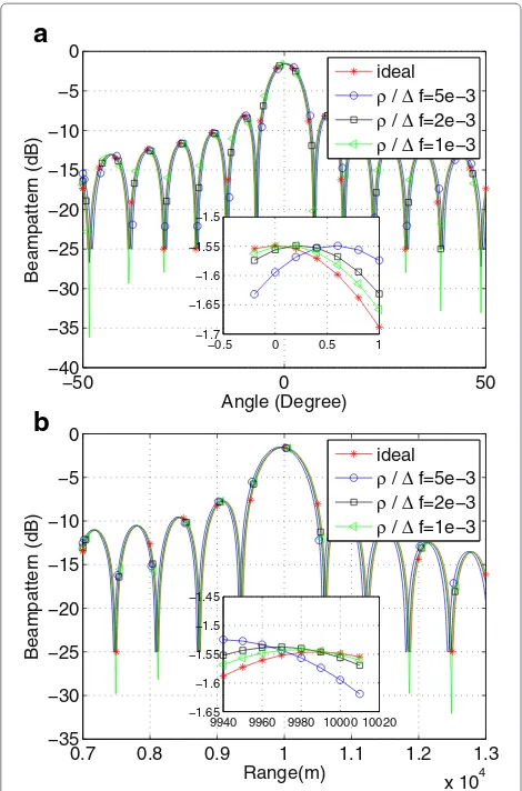
Figure 3a,b shows the FDA beampattern with uniform frequency increment errorsρ, frequency incrementf =
30 KHz, andt = 1/f. It can be noticed that the phase error forθ = 0.5◦isρ/f = 5×10⁻³. Note that since the range attenuation exists, the range error has a small deviation from the calculation of Equation 21.
4 Impacts of stochastic frequency increment
errors
In this section, we investigate the statistical properties of FDA beampattern with random frequency increment errors.
4.1 Error boundary of FDA beampattern
Suppose the frequency increment errors are random. In this case, it is not possible to derive a deterministic beam-pattern expression like Equation 17. Here, we are inter-ested in the maximum beampattern deviation, namely:
max
t,r,θ |A(t,r,θ)|. (23)
According to Equation 16 and using the Cauchy-Schwarz inequality, we have:
max
t,r,θ |A(θ,r,t)| ≤ 1
−50 0 50
9940 9960 9980 10000 10020 −1.65
Figure 3FDA beampattern profiles with frequency increment errors. (a)In angle dimension.(b)In range dimension.
= 1
where|·|and · 2denote the absolute value and Euclidean norm, respectively, andwmaxdenotes the maximum ele-ment of w. Note that compared with [29], |wmax| ≤ |w|2, the bound expressed in Equation 24 is much tighter. According to Equation 16,C+can be rewritten as:
C+ 2=
The maximum deviation, in a linear scale, is the same over the whole beampattern. When only C+ (and thusC) is known, or when the influence of unknown factors onC+,
e.g., aging or temperature, comes into play, it makes sense to consider as random matrix, with some statistical model for the entries ofC+. We then have to calculate:
max C+ 2 (26)
for the random matrixC+to find an upper bound.
max C+ 2=max 2π
When applying this result to an array with uniform weightingwmax=1, Equation 24 leads to:
Amax= frequency increment error will become amplitude error of FDA beampattern, as shown follows:
Amax=
It can be noticed from Equation 29 that the errors caused by time and by range counterbalance the total beampattern error. Therefore, we delete 1/f. Then, Equation 29 can be reformulated as:
Amax≤
Equation 30 gives FDA beampattern error bound which indicates its worst case. Since it is caused by the frequency increment errors, the maximum device errors which pro-duce the FDA frequency increment are regulated by the bound. This gives guideline about device selections and predicts the possible FDA beampattern derivation bound.
4.2 Statistical properties of FDA beampattern
4.2.1 Expected value
Using Equations 8 and 13, it is straightforward to show that:
E{A(θ,r,t)} =EwHC(r,t)v(θ,r,t)−wHv(θ,r,t)
=wHE{C(r,t)}v(θ,r,t)−wHv(θ,r,t)
(31)
whereE{·}denotes the expected value.
Assume that the frequency increment errorρn of the
nth element satisfies the Gaussian statistical modelρn ∼
N(0,σ2)and the PDF is as follows:
Therefore, the expected value of the nth element in diag(C)can be calculated as [30]: applying Equation 33 onto 31, we can get the expected value of FDA beampattern deviation with Gaussian distri-bution frequency increment errors as follows:
E{A(θ,r,t)} =wHE{C(r,t)}v(θ,r,t)−wHv(θ,r,t)
andIdenotesN×Nunit matrix. In this case, the expected value of the FDA beampattern deviation is dependent on the variance of frequency increment errors and is not 0 for the Gaussian distribution model.
For another case, we assume that ρn is uniform dis-tribution, i.e., ρn ∼ u(−ρmax,ρmax) with minimum
and maximum values −ρmax andρmax. We can get the expected value ofnth element in diag(C)as follows:
E{Cnn(r,t)} =E
By using Equation 36 onto 31, the expected value of FDA beampattern deviation with uniform distribution frequency increment error can be reformulated as:
E{A(θ,r,t)} =wHE{C(r,t)}v(θ,r,t)−wHv(θ,r,t)
Similarly, the expected value of the FDA beampattern deviation is dependent on the maximum value of fre-quency increment error and not 0 for the uniform distri-bution model. From Equations 34 and 37, the expected values of FDA beampattern have range offset and angle offset, which is caused by time dependent error on the two distributions.
4.2.2 Variance
The beampattern deviation variance var{A(θ,r,t)}
equals to the beampattern variance:
var{A(θ,r,t)} =var{A(θ,r,t)}
=varwHC(r,t)v(θ,r,t). (39) As we deal with vectors and matrices, we utilize the covariance matrix cov{·}, and var{·} = cov{·} for any scalar. We thus have:
var{A(θ,r,t)} =covwHC(r,t)v(θ,r,t) (40)
Using the Kronecker product⊗, the vectorization trans-formation vec(·)and the identity:
vec{ABC} =CT⊗Avec{B}. (41)
Since
we use c = vec{C(r,t)} and the vector t(θ,r,t) = vT(θ,r,t)⊗wH, which utilizing:
cov{AX} =Acov{X}AH (43)
to yield:
var{A(θ,r,t)} =t(θ,r,t)cov{c(r,t)}tH(θ,r,t). (44)
SinceCis a diagonal matrix and its entries are indepen-dent random variables, cov(c)is a diagonal matrix and has non-zero value with thenNth entry. We then have:
var{A(θ,r,t)} = general result that we can evaluate and review for different statistical models for cov{c(r)}kk.
Assume that all the random frequency increment errors have the same distribution. For the first case, frequency increment errorρnof thenth element satisfies the Gaus-sian statistical model ρn ∼ N(0,σ2). According to the Equations 13 and 36, 46 can be rewritten as:
cov{c(r,t)}kk=
where [·]∗ denotes the conjugate operator. Here, the
E(C(r,t)nn)=e−2π lized. Applying Equation 32, the first term of Equation 47 can be rewritten as:
+∞
Applying it to Equation 47 yields:
cov{c(r,t)}kk=1−E(C(r,t))2nn distinguish from n. Consequently, we can get the FDA beampattern deviation variance:
var{A(θ,r,t)} =
Similarly, we can get the FDA beampattern variance with the random frequency increment errors, which are uniformly distributed as aforementioned:
var{A(θ,r,t)} =
Compared with Equations 50 and 51, we can see that the FDA beampattern variances at both kinds of random frequency increment error distributions are dependent on the statistics properties. Given the same frequency incre-ment errors, the variances will decrease when the number of elements is increased.
4.2.3 PDF
derive the PDF of beampattern based on the PDF of the frequency increment errors.
For the first case, we investigate the PDF of beampattern when the frequency increment errors obey the Gaussian distribution as aforementioned. According to Equation 13, we derive the PDF ofC. It is known that: part and imaginary part of Cnn, respectively. Conse-quently, we have:
ρ= arcsin(imag(Cnn)) derivation operation. We have:
fgn(gn)=fρ[h(gn)]h(gn) can be rewritten as:
˜
r for notation convenience, we can find % Equation 57, we can get:
g2cosϕ+ %
1−g22sinϕ=a2. (58)
Solving Equation 58, it yields:
g2=a2cosϕ+sinϕ
denotes the imaginary part of ˜
The joint PDF of the variables above is as follows:
fA˜ig3...gN(A˜ig3. . .gN)
According to Equations 59 and 60, we can get that:
J=
. Since the each element ofCis
responding to only one frequency increment error which is random and independent,gn is the independent with othergmwithm=1, 2,. . .,N−1 andm=n. Therefore, Equation 61 can be rewritten as:
Moreover, we can get the PDF of FDA beampattern as:
fA˜
i(A˜i)= 1
−1 . . .
1
−1
fg2g3...gN
ξ2(A˜i(θ,r,t)),ξ3(g3),. . .,ξN(gN)
×
⎛ ⎜
⎝cosφ−%sinφ
1−a22
⎞ ⎟
⎠dg3. . .dgN.
(64)
Utilizing the same approach, we can get the PDF of real part of FDA beampattern. Since the relationship between real part and imaginary part is complex, so we cannot give the PDF of the whole FDA beampattern.
Similarly, we can derive the FDA beampattern variance with the random frequency increment errors, which are uniformly distributed as aforementioned. The PDF ofgnis as follows:
fgn(gn)=fρ[h(gn)]h(gn)
= 1
2ρmax
1
2π(n−1)t−cr 0
$ 1−g2
n ,
−1<gn<1
(65)
and the PDF of FDA beampattern imaginary part is as follows:
fA˜
i(A˜i)= 1
−1 . . .
1
−1
fg2g3...gN
ξ2(A˜i(θ,r,t)),ξ3(g3),. . .,ξN(gN)
×
⎛ ⎜
⎝cosφ−%sinφ
1−a22
⎞ ⎟
⎠dg3. . .dgN.
(66)
5 Simulation results
5.1 Example 1: FDA beampattern bound
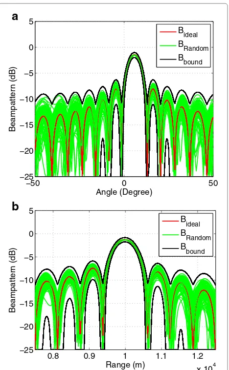
Consider a 16-element uniform linear FDA with half of wavelength λ spacing between neighbor elements. The center frequency f0 is 10 GHz, and the increment fre-quencyf is 30 KHz. The target is located at the range 10 km, angle 0◦, and the time is on 1/f. Figure 4a,b shows the comparisons of ideal FDA beampatternBideal, FDA beampattern upper and lower bound Bbound, and FDA beampattern with random frequency increment errorsBRandom. In the FDA beampattern with random fre-quency increment errors, the frefre-quency increment errors are Gaussian distribution, i.e., ρn ∼ N(0, 902) and the random FDA beampatterns are based on 50 indepen-dent Monte Carlo simulation runs. It can be shown that the present bounds hold for all the simulated beampat-tern realizations for both Figure 4a,b. Simulations results show that the bounds are tighter in range dimension than
−50 0 50
−25 −20 −15 −10 −5 0 5
Angle (Degree)
Beampattern (dB)
Bideal
BRandom
B
bound
0.8 0.9 1 1.1 1.2 x 10⁴ −25
−20 −15 −10 −5 0 5
Range (m)
Beampattern (dB)
Bideal
BRandom
Bbound
a
b
Figure 4Profiles for the ideal, the bounds, and the errors FDA beampattern.(a)In angle dimension.(b)In range dimension.
that in the angle dimension which is caused by range counterbalance of the total error in beampattern.
10
−110
010
110
2−250
−200
−150
−100
−50
σ
Beampattern error (dB)
Theoretical
Empirical
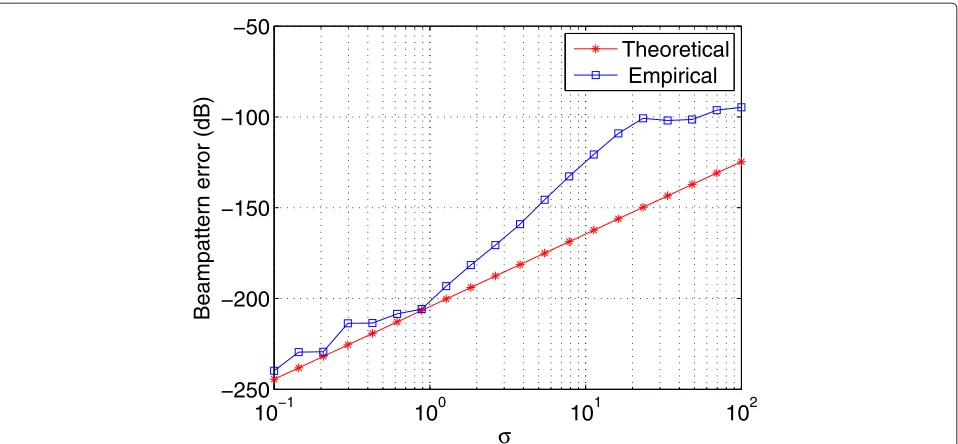
Figure 5The comparison of Gaussian random FDA beampattern error expectation value.
5.2 Example 2: FDA beampattern PDF
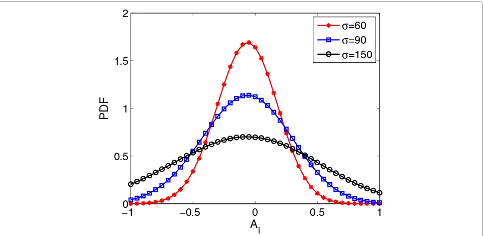
Consider a uniform linear FDA with four elements. In this example, FDA beampattern amplitude error does not divide into the factorr0, and its value is very large com-pared with that of Figures 5 and 6. Other array parameters are the same to that of example 1. Figure 7 shows PDFs of theoretical and empirical results, and Figure 8 shows the PDFs of imaginary part of random FDA beampat-tern with different σs. It can be known that lower σ
enjoys the smaller beampattern errors, and PDF curves are centrosymmetric with the center aboutAi = 0. One might use this figure and Equation 64 to specify toler-ance requirements of frequency increment errors to fulfill a given beampttern requrement with certain probability. For instance, if probability of the beampttern errors at the domain (−0.5 to 0.5) is not smaller than 0.95, the standard deviations of ρ for every elements of FDA array will be required to be no larger than 60.
10
−110
010
110
2−110
−100
−90
−80
−70
−60
−50
−40
σ
Beampattern error (dB)
Theoretical
Empirical
−10 −0.5 0 0.5 1 0.2
0.4 0.6 0.8 1 1.2 1.4
A
i
Theoretical Empirical
Figure 7The PDF of Gaussian random FDA beampattern error.
6 Conclusions
In this paper, we have investigated the impacts of fre-quency increment errors on FDA beampattern based on deterministic errors and random errors. For uniform and linear deterministic frequency increment errors, the spe-cific beampattern error formulations are provided, which gives guideline for device selection. For the stochastic fre-quency increment errors, we have derived a very tight
worst-case boundary of the FDA beampattern. Simulation results show that all the random beampatterns are held for the derived bounds, and the worst-case boundary is help-ful to the FDA system design. At last, we derived the sta-tistical properties of the expectation, variance, and PDF. They can be used to analyze the probability of FDA beam-pattern fluctuations for the given distribution frequency increment errors.
−10 −0.5 0 0.5 1
0.5 1 1.5 2
A
i
σ=60
σ=90
σ=150
Competing interests
The authors declare that they have no competing interests.
Authors’ contributions
All authors formulated and discussed the idea together. Additionally, KG wrote the paper. All authors read and approved the final manuscript.
Acknowledgements
This work was supported in part by the Program for New Century Excellent Talents in University under grant no. NCET-12-0095.
Received: 3 November 2014 Accepted: 12 March 2015
References
1. BDV Veen, KM Buckley, Beamforming: a versatile approach to spatial filtering. IEEE ASSP Mag.5(2), 4–24 (1988)
2. J Xie, H Li, Z He, C Li, A robust adaptive beamforming method based on the matrix reconstruction against a large doa mismatch. EURASIP J. Adv. Signal Process.2014(91), 1–10 (2014)
3. P Antonik, MC Wicks, HD Griffiths, CJ Baker, inProceedings of the IEEE Radar Conference. Frequency diverse array radars (IEEE, Verona, NY, 2006), pp. 215–217
4. MC Wicks, P Antonik,Frequency diverse array with independent modulation of frequency, amplitude, and phase. in January 15, 2008. (U.S.A Patent 7,319,427, USA)
5. P Antonik, MC Wicks,Frequency diverse array with independent modulation of frequency, amplitude, and phase. in June 5, 2008. U.S.A Patent 7, Application 20080129584, USA
6. P Antonik, MC Wicks,Method and apparatus for a frequency diverse array. in March 31, 2009. U.S.A Patent 7.511, 665B2, USA
7. P Antonik, An investigation of a frequency diverse array. PhD thesis, University College London (2009)
8. S Brady, Frequency diverse array radar: signal characterization and measurement accuacy. PhD thesis, Air Force Institute of Technology (2010)
9. M Secmen, S Demir, A Hizal, T Eker, inProceedings of the IEEE Radar Conference. Frequency diverse array antenna with periodic time modulated pattern in range and angle (IEEE, Boston, MA, 2007), pp. 427–430
10. P Baizert, TB Hale, MA Temple, MC Wicks, Forward-looking radar GMTI benefits using a linear frequency diverse array. Electron. Lett.42(22), 1311–1312 (2006)
11. C Cetintepe, S Demir, Multipath characteristics of frequency diverse arrays over a ground plane. IEEE Trans. Antennas Propagation.62(7),
3567–3574 (2014)
12. J Shin, J-H Choi, J Kim, J Yang, W Lee, J So, C Cheon, inMicrowave Conference Proceedings (APMC). Full-wave simulation of frequency diverse array antenna using the FDTD method (IEEE, Seoul, Korea, 2013), pp. 1070–1072
13. T Eker, S Demir, A Hizal, Exploitation of linear frequency modulated continuous waveform (LFMCW) for frequency diverse arrays. IEEE Trans. Antennas Propagation.61(7), 3546–3553 (2013)
14. YB Wang, WQ Wang, HZ Shao, Frequency diverse array Cramér-Rao lower bounds for estimating direction, range and velocity. Int J Antennas Propagation.2014, 1–10 (2014)
15. V Ravenni, inProceedings of the 4th European Radar Conference. Performance evaluations of frequency diversity radar system (IEEE, Munich, Germany, 2009), pp. 436–439
16. L Zhuang, XZ Liu, Application of frequency diversity to suppress grating lobes in coherent MIMO radar with separated subapertures. EURASIP J. Adv. Signal Process.2009, 1–10 (2009)
17. WQ Wang, Phased-MIMO radar with frequency diversity for range-dependent beamforming. EURASIP J. Adv. Signal Process.13(4), 1320–1328 (2013)
18. W-Q Wang, HZ Shao, Range-angle localization of targets by a
double-pulse frequency diverse array radar. IEEE J. Sel. Top. Signal Process.
8(1), 106–114 (2014)
19. W-Q Wang, HC So, Transmit subaperturing for range and angle estimation in frequency diverse array radar. IEEE Trans. Signal Process.
62(8), 2000–2011 (2014)
20. E Yazdian, S Gazor, MH Bastani, Limiting spectral distribution of the sample covariance matrix of the windowed array data. EURASIP J. Adv. Signal Process.2013(42), 1–15 (2013)
21. J Xie, Z He, H Li, J Li, 2D DOA estimation with sparse uniform circular arrays in the presence of mutual coupling. EURASIP J. Adv. Signal Process.
2011(127), 1–18 (2011)
22. M Khodja, A Belouchrani, K Abed-Meraim, Performance analysis for time-frequency music algorithm in presence of both additive noise and array calibration errors. EURASIP J. Adv. Signal Process.2012(94), 1–11 (2012) 23. Y Han, D Zhang, A recursive Bayesian beamforming for steering vector
uncertainties. EURASIP J. Adv. Signal Process.1(108), 1–10 (2014) 24. S Henault, SK Podilchak, SM Mikki, YMM Antar, A methodology for mutual
coupling estimation and compensation in antennas. IEEE Trans. Antennas Propagation.61(3), 1119–1132 (2013)
25. H Chen, B Liu, P Huang, J Liang, Y Gu, Mobility-assisted node localization based on TOA measurements without time synchronization in wireless sensor networks. MONET.17(1), 90–99 (2012)
26. H Chen, G Wang, Z Wang, H-C So, HV Poor, Non-line-of-sight node localization based on semi-definite programming in wireless sensor networks. IEEE Trans. Wireless Commun.11(1), 108–116 (2012) 27. H Chen, Q Shi, R Tan, HV Poor, K Sezaki, Mobile element assisted
cooperative localization for wireless sensor networks with obstacles. IEEE Trans. Wireless Commun.9(3), 956–963 (2010)
28. W Zhang, Q Yin, H Chen, F Gao, N Ansari, Distributed angle estimation for localization in wireless sensor networks. IEEE Trans. Wireless Commun.
12(2), 527–537 (2013)
29. CM Schmid, S Schuster, R Feger, A Stelzer, On the effects of calibration errors and mutual coupling on the beam pattern of an antenna array. IEEE Trans. Antennas Propagation.61(8), 4063–4071 (2013) 30. H Chen, F Gao, MH Martins, JL P Huang, Accurate and efficient node
localization for mobile sensor networks. MONET.18(1), 141–147 (2013)
Submit your manuscript to a
journal and benefi t from:
7Convenient online submission
7Rigorous peer review
7Immediate publication on acceptance
7Open access: articles freely available online
7High visibility within the fi eld
7Retaining the copyright to your article