Two dimensional SLIM with application to pulse Doppler MIMO radars

R E S E A R C H

Open Access

Two-dimensional SLIM with application to

pulse Doppler MIMO radars

Mohammad Jabbarian-Jahromi

and Mohammad Hossein Kahaei

Abstract

A two-dimensional (2D) sparse signal model is developed for pulse Doppler MIMO radars. Using this model, we develop the 2D sparse learning via iterative minimization (2D SLIM) algorithm. Simulation results show that the 2D SLIM compared to the 1D SLIM drastically reduces the computational burden while both of them have the same performance. Also, for estimation of range-angle-Doppler parameters, the 2D SLIM outperforms the matched filter (MF), smoothed L0-norm (SL0), iterative adaptive approach (IAA), and spectral projected gradient forl1-norm minimization (SPGL1) algorithms.

Keywords:Pulse Doppler MIMO radar; Sparse learning via iterative minimization; Two-dimensional sparse signal model

1 Introduction

Multiple-input multiple-output (MIMO) radars by exploit-ing multiple transmitters and receivers have recently been introduced [1–3]. It is well known that in this structure due to making use of orthogonal (or highly uncorrelated) transmit signals, the received signals can easily be sepa-rated. MIMO radars are often divided into two categories based on antenna placement. In the first one, the transmit and receive antennas are widely separated, and thus, the targets are observed from different directions dealing with target fluctuation fading [4–7]. In the second category, however, antennas are collocated so that the different phases from received signals can be extracted by the re-ceivers. In this case, due to the waveforms diversity, a higher spatial resolution is achieved compared to the trad-itional radars. Also, in MIMO radars, target detection and parameter estimation are improved by suitably de-signing transmit beam-pattern [8–13]. Here, we consider the second structure.

From a sparsity perspective, in most radar applica-tions, the number of targets located in the radar surveil-lance area is much smaller than the whole number of range-angle-Doppler bins. Thus, a sparse model can be derived for the received signal, and accordingly sparse signal recovery algorithms can be used for estimating

the target parameters including range, Doppler fre-quency, and angle [14–18]. The aim of using sparse so-lution in a radar system is to more accurately estimate the target parameters compared to the traditional methods such as matched filters (MF).

Compressed sensing (CS), which is rooted on the princi-ples of sparsity theory, has recently received considerable attention in MIMO radars [19–21]. Although, the main goal of the CS problem is to reduce the sampling rate lower than the Nyquist criterion, here we mainly focused on achieving accurate estimates for target parameters with much lower computations. For this purpose, an efficient technique is the sparse learning via iterative minimization (SLIM) algorithm which is computationally simple com-pared to the iterative adaptive approach (IAA) and focal underdetermined system solver (FOCUSS) algorithms due to the use of the conjugate gradient least squares (CGLS) algorithm [22]. This algorithm, which is a 1D algorithm (or namely 1D SLIM), is a maximuma posteriori(MAP) estimator which maximizes a posteriori Bayesian model. An important characteristic of 1D SLIM is incorporation oflq-norm optimization (0 <q≤1) in comparison with the l1-norm in order to reach sparser solutions and more

ac-curate estimates. In [22], the 1D SLIM has been developed for MIMO radars by using only one pulse. Based on [22], this algorithm estimates a sparser vector compared to the l1-norm algorithm. On the other hand, the smoothed L0

(SL0) algorithm has been presented for two-dimensional

* Correspondence:[email protected]

Signal & System Modeling Lab., School of Electrical Engineering, Iran University of Science and Technology, Tehran 16846-13114, Iran

(2D) sparse problems [23]. In this algorithm, a discontinu-ous l0-norm function is approximated by a continuous

one and then a sparse solution is reached using the stee-pest ascent algorithm followed by a projection onto a feas-ible set [24–27]. In [28], this algorithm has been applied to pulse Doppler radars with a lot of advantages such as tar-get velocity extraction and pulse integration. However, this algorithm has been presented by using an approximated l0-norm function for which we will later show that it

achieves a lower performance in sparse signal recovery at low signal-to-noise ratios (SNRs) or for a small number of pulses compared to the SLIM algorithm. Also, the 2D IAA which is a nonparametric algorithm is presented in [29] for a general sparse solution. However, as it will be shown in the simulation section, its performance is poor at low SNRs and also for a small number of pulses.

In [30], a low-complexity CS approach is developed by decoupling the range, Doppler frequency, and angle pa-rameters. It is assumed that the estimates of azimuth an-gles are obtained from one pulse by discretizing the angle space. Then, the Doppler estimates are extracted by combining the data of multiple pulses and using the initial estimated angles. Based on angle-Doppler esti-mates, the range is then estimated using frequency-varying received pulses. However, two problems are still of concern. First, the number of targets within the radar surveillance area is, in practice, so large that the angle space will not be sparse enough to apply the CS theory. In addition, a huge number of antennas are needed in a MIMO radar to discriminate among a large number of targets in the angle space with an acceptable resolution. Secondly, the SNR of one pulse is not sufficient for esti-mation of targets’angles.

In this paper, we develop a 2D sparse model for pulse Doppler MIMO radar signals and find its relation with the Kronecker product factorization in the 1D model. To solve the 2D sparse signal equation, it can be converted to a 1D model and be recovered using 1D sparse recovery al-gorithms. However, this leads to a very large number of computations for which we will introduce here a new sim-pler technique. Therefore, a 2D SLIM algorithm is pro-posed for direct solution of a 2D sparse signal equation. In this approach, the Kronecker factorization is used to sep-arate a large-dimension matrix into two smaller matrices. This procedure leads to reducing the number of products and therefore decreasing the computation cost and re-quired memories.

Moreover, we develop the 2D version of the well-known 1D matched filter (1D MF) for comparison with the pro-posed 2D SLIM. Moreover, we compare the 2D SLIM al-gorithm with spectral projected gradient for l1-norm

minimization (SPGL1) algorithm which is appropriate for large-scale sparse recovery problems and complex-valued data [31].

The paper is organized as follows. In Section 2, in a common scenario for aircraft surveillance MIMO radar in which the intra-pulse Doppler shift is negligible, a 2D-sparse model is developed. To solve this 2D sparse signal equation, in Section 3, the 2D SLIM and 2D MF algorithms are derived. The computational complexities of 1D and 2D SLIM algorithms are discussed in Sec-tion 4. Using simulaSec-tion results in SecSec-tion 5, computa-tional complexities and the performances of different algorithms are compared, and Section 6 concludes the paper. The list of notations used in this work is shown in Table 1.

2 Signal model for pulse Doppler MIMO radars

Figure 1a shows a typical radio frequency (RF) transmit pulse train of a pulse Doppler radar in whichτis the pulse width. For the received signals, two different scenarios may be considered for extraction of the Doppler shift/fre-quency,fd[32, 33]. In a general scenario shown in Fig. 1b, τandfdare large enough to havefdτ> 1, for which at least one period offdlies within the receive pulse width. How-ever, in the second scenario shown in Fig. 1c, we havefdτ < 1 (usuallyfdτ< < 1), in which case several pulses are re-quired to extractfd. This scenario; which we have consid-ered in this work, is commonly encountconsid-ered in aircraft surveillance radars [32]. In this scenario, the effect of the Doppler frequency on each pulse is negligible and may be viewed as the sampling of the Doppler signal by the radar pulse repetition frequency (PRF),fr.

The data model and problem formulation for Fig. 1c are presented as follows. As shown in Fig. 2, the trans-mit signal is a train ofNP probing pulses each of which containingNs sub-pulses with the bandwidthB. We as-sume that the targets are located behind the maximum unambiguous ranges with no ambiguity in the Doppler

frequency interval of interest −fr

2 ; fr

2

h

. This interval is

di-vided intoNDDoppler bins as

Table 1List of notations ‖.‖2 l2-norm

‖.‖F Frobenius norm of matrix

⊙ Hadamard (element-wise) matrix product

⊗ Kronecker product

(⋅)T Transpose of a vector or matrix

(⋅)H Conjugate transpose of a vector or matrix

(⋅)* Conjugate of a vector or matrix

⊘ Element-wise matrix division

⋅ ð Þc

i ith column of a matrix

⋅ ð Þr

i ith row of a matrix

fd¼−

fr 2 þ

frðd−1Þ

ND ; d

¼1;2;⋯;ND: ð1Þ

Now, we calculate the amount of phase shift over one sub-pulse caused by the Doppler phenomenon. Thus, for the dth Doppler bin, the Doppler phase shift over one sub-pulse can defined as

ωd¼ 2πfd

B ; d¼1;2;⋯;ND: ð2Þ

By considering the waveform for sub-pulsessi∈ℂ1Ns; i= 1,…,Mt as the code sequence of the ith transmit antenna, transmit signals are defined by an Mt×Ns matrix as

S¼ sT

1 sT2 ⋯sTMt

h iT

: ð3Þ

Also, the range dimension of surveillance area is di-vided into NR bins. Accordingly, the largest possible delay between the transmit and receive pulses isNR−1.

Then, the transmitted pulse waveforms can be arranged into the matrixS~;so that

~

S¼ S 0MtðNR−1Þ

ð4Þ

where0M_tðNR−1Þ is anMt× (NR−1) matrix of zeros, and

we haveS~∈ℂMtðNsþNR−1Þ_{. Also, we assume that the}

an-gular interval of interest θa is divided into _NA angular bins (a= 1,⋯,NA). Then, in a uniform linear array, the steering vectors ofMttransmit and Mrreceive antennas are respectively denoted by

aa¼

1 e−

j2πΔtsinð Þθa

λ0 _{⋯ e}−

j2πðMt−1ÞΔtsinð Þθa λ0

" #T

ð5Þ

and

(a)

(b)

(c)

Fig. 1aA typical RF transmit pulse train of a pulse Doppler radar;bandcreceived signals in baseband forfdτ> 1 (general scenario) andfdτ< 1

(common scenario for aircraft-surveillance radar), respectively [32]

ba¼

where λ0 is the radar carrier wavelength and Δt andΔr

show the distances between two adjacent transmit and receive antennas, respectively. Therefore, the pth re-ceived pulse matrixYp∈ℂMrðNsþNR−1Þcan be written as

whereΕpis the additive white Gaussian noise matrix for the pth pulse (p= 1, 2,⋯,NP),TR is the ratio of pulse repetition interval (PRI) over the single sub-pulse dur-ation, and d= 1,⋯,NDdenote the return complex reflection coeffi-cients of targets corresponding to the radar cross-section. In this scenario, since the number of range-angle-Doppler bins, in which actual targets are detected, is much smaller than the total number of radar bins, most of reflection coefficients are zero, and thus, the radar sig-nal model can be assumed sparse. We assume that complex reflection coefficients during pulse repetitions are constant.

We will show that (7) can be converted to a 2D sparse from in which the unknown parameters αr,a,d are pre-sented in matrix form. By defining and using

v_r;a¼vec baaTaSJ~ r

where ep= vec(Ep) is a complex Gaussian noise vector with zero mean and covariance matrixI. Equivalently, in a more compact form, we get

y_p¼AXθpþep ð13Þ

where X¼½x1 ⋯ xND contains the complex

reflec-tion coefficients corresponding to the radar cross-section, andθp¼ ejTRðp−1Þω1 ⋯ ejTRðp−1ÞωND

Equation (14) presents a 2D sparse signal model for pulse Doppler MIMO radars whereY∈ℂMrðNsþNR−1ÞNP;

A∈ℂ½MrðNsþNR−1Þ½NRNA;Θ∈ℂNDNP;_andX∈ℂNRNAND_.

Due to the underdetermined nature of (14) for a sparse model (i.e., Mr(Ns+NR−1) <NRNA andNP<ND), it has no unique solution. Our goal is to find the sparsest matrix forXin which we have as many zero elements as possible.

The 2D sparse signal model given by (14) can be con-verted to a 1D model by using the following property [34]:

vecðAXΘÞ ¼ ðΘT⊗AÞvecð ÞX :

ð15Þ

Therefore, we have

y¼Φxþe; ð16Þ

wherex= vec(X),y= vec(Y),e= vec(E), andΦ=ΘT⊗A. Although x can be computed using 1D sparse recovery algorithms such as IAA [35] and SLIM [22], due to the large dimension of Φ∈ℂ½NPMrðNsþNR−1Þ½NRNAND;_1D

so-lutions are computationally extremely expensive. Ac-cordingly, due to the smaller number of products appeared in (14) compared to (16), developing the 2D al-gorithm for direct solution of (14) leads to an extreme reduction of computational load compared to 1D one.

3 2D sparse signal recovery

In this section, at first, we give an overview of 1D SLIM algorithm. Then, a 2D SLIM algorithm is proposed for pulse Doppler MIMO radars by direct solution of (14), which leads to a lower computational cost compared to the 1D algorithms. In addition, for comparison purposes, the 2D SLIM is compared with the 2D SL0 [23] and 2D IAA [29] algorithms recently introduced for 2D sparse recovery problems. Moreover, we develop the 2D MF for comparison purposes.

3.1 Overview on 1D SLIM algorithm

fð Þ ¼x Y

N

n¼1

e−2qðj jxnq−1Þ ð₁₇Þ

whereqis a free parameter between 0 <q≤1,xnis thenth component of vectorx, andN=NRNAND. The above prior can lead to a more accurate estimation of the sparse vec-torx. Whenq→0, this prior will have a sharper peak at 0 and thus causes sparser estimates in the Bayesian infer-ence. For q= 1, this prior will be similar to the Laplace prior fð Þx ∝e−k kx1 with finite peaks at 0. By assuming an

independent and complex Gaussian distribution with zero mean and varianceηIfor additive noisee, the conditional distribution for measurement data vectorycan be defined as fðyjx;ηÞ ¼ CNðAx; ηIÞ. By assuming a uniform prior forηasf(η)∝1, the cost function for the SLIM based on the MAP approach is defined as

max logarithm of (18), the cost function will be equivalent to

Jðx;ηÞ ¼Klogηþ1

By minimizing (19) with respect to xandηand using a heuristic approach, an iterative solution is obtained for the 1D SLIM in two steps [22]:

1. Iterative estimation of sparse vectorx,

xðtþ1Þ_¼Πð Þt _ΦH_ΦΠð Þt _ΦH_þηð Þt_I−1_{y ð20Þ}

where the superscript t shows the iteration number,

Π= diag{ϑ}, and ϑn= |xn|2−q, n= 1,⋯,NRNAND, ϑn is the nth component of vector ϑ.

2. Iterative estimation of noise powerη,

ηðtþ1Þ_¼ 1

Our aim in this subsection is to develop the 2D version of (20) and (21) usingΦ=ΘT⊗A and (14) and follow-ing Hadamard matrix property:

diag vecf ð ÞA gvecð Þ ¼B vecðA⊙BÞ: ð22Þ

Since matrix inversion in (20) has an extreme computa-tional load, we propose to use the conjugate gradient least

square (CGLS) algorithm [36] to solve (14) with lower computations. To do so, by defining the vector u= (ΦΠΦH+ηI)−1y, the 2D CGLS is derived in the Appendix as summarized in Table 2. Note that the superscriptthas been suppressed for simplicity and the components of matrixΣareΣij=Γij1/2where

Γij¼ Xij 2−q

i¼1;⋯;NRNA; j¼1;⋯;ND: ð23Þ

To derive the 2D SLIM, the relationship between Π andΓcan be presented as

Π¼diag vecf ð ÞΓ g ð24Þ

where the elements ofΓ are given by (23). By substitut-ing (24) andΦ=ΘT⊗Ain (20), we obtain

x¼diag vecf ð ÞΓ gðΘT⊗AÞHu:

ð25Þ

Then, by using the Kronecker product property [37]

Θ⊗A

ð ÞH _¼ΘH_⊗AH _ð26Þ

and using (15) and (22), (25) is shown as

x¼vecΓ⊙AHUΘH ð27Þ

where U∈ℂMrðNsþNR−1ÞNP _{is obtained by the 2D CGLS}

algorithm as presented in Table 2 and u= vec(U). Note that X=Γ⊙(AHUΘH), and thus for the (t + 1)th iter-ation of step 1 of the 2D SLIM, we have

Xðtþ1Þ_¼Γð Þt_⊙AH_Uð Þt _ΘH_{: ð28Þ}

Also, from (14) and (16), we can easily express step 2 of the 2D SLIM as

Table 22D CGLS Algorithm

ηðtþ1Þ_¼ 1

For initialization of the 2D SLIM, i.e., X(0), we make use of minimum l2-norm solution using the

economy-size QR decomposition [28] by incorpor-ation of a hard threshold operator in order to spar-sify X(0). The required criterion for stopping the 2D SLIM recursion is developed based on the 1D ver-sion [22] as

whereΔis a small positive constant.

The parameterqplays an important role in sparse sig-nals recovery using the SLIM. For _q→0, it achieves a sparser solution compared to the case whenq→1; how-ever, it is hard to determine the sparsity level. To cope with this problem, _q can be estimated appropriately by the Bayesian information criterion (BIC) [22] given by

BICq¼2MrNPðNSþNr−1Þ log Y−AX^Θ 2 F

þ5h qð Þ ln 2ð MrNPðNSþNr−1ÞÞ ð31Þ

where h(q) is the number of selected peaks in the output of the SLIM algorithm that is executed for a particular value ofq. To explain how we choose the number of se-lected peaks (h(q)), at first, the absolute value of the SLIM algorithm output defined as |X| is sorted in a descending order. Then, the largest peak is selected and the other values of matrix Xare set to zero to form the matrix X^.

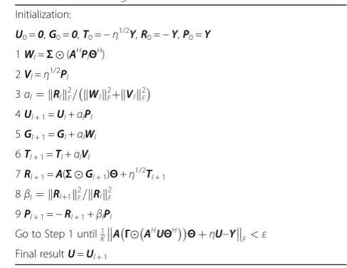
Fig. 4MIMO radar Doppler-angle estimates for targets that fall on grid points (Nt= 40, SNR = 10 dB) foraMF,bSL0,cSPGL1,dIAA, andeSLIM

round, the two largest peaks are selected and the other values of X are set to zero, and the related BIC is com-puted for X^ andh(q) = 2 and so on. The value ofh(q) is the number of the selected peaks that yields the lowest BIC. After running the 2D SLIM for a selected set of q and computing h(q), we choose that q which minimizes the BIC. The factor 5 in (28) shows the number of un-known parameters including range, angle, Doppler fre-quency, and the complex reflection coefficients of targets.

3.3 2D MF

The 1D MF output has already been derived for MIMO radars as [22]

Noting that the columns ofΦ are defined by the vec-torsð ÞΦ c_n; n¼1;2;…;NRNAND and using Φ=ΘT⊗A and (26), the numerator of (32) is obtained as

ΦH_y¼vecAH_YΘH_{: ð33Þ}

Next, the denominator of (32) is shown by using the Kronecker product properties as

Φ ND. By substituting (33) and (34) in (32) and converting to the 2D form, we obtain the 2D MF as

X¼AH_YΘH_{⊘Λ ð35Þ}

where the elements of Λ∈ℂNRNAND _{are defined by} Λ

ij and⊘is the element-wise matrix division.

4 Computational complexity of 1D and 2D SLIM

In the 1D SLIM, the main computational cost in each it-eration belongs to the product ofΦ and a vector likex. For the 2D SLIM, this product is converted to a 2D form asAXΘusing the Kronecker factorizationΦ=ΘT⊗A.

The main difference between the 1D and 2D forms from a computational point of view is in the number of flops

(a)

(b)

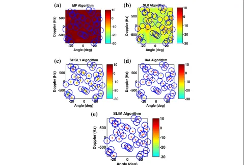
Fig. 5MIMO radar Doppler-range estimates for targets that fall on grid points (Nt= 40, SNR = 10 dB) foraMF,bSL0,cSPGL1,dIAA, andeSLIM

for calculatingΦxandAXΘ. The complexities ofΦxand AXΘ are O(NPMr(Ns+NR−1)NRNAND) and O(Mr(Ns+ NR−1)NRNAND) +O(NPMr(Ns+NR−1)ND), respectively. We have assumed that the product matrix AX is com-puted first, and then the result is multiplied byΘ. By com-paring these two computational complexities, it is demonstrated that the ratio of the 2D processing load over that of its equivalent 1D is _N1

Pþ

1

NRNA. If it is assumed

NP≪NRNA, then this ratio is equal to_N1

P.

In addition, the Kronecker factorization can take ad-vantage of multi-core processors [38] by which the 2D SLIM algorithm can be parallelized and solved. Then, the speed of this algorithm compared to the 1D one is approximately increased by a factor proportional to the number of processing cores.

5 Numerical examples

To show the computational efficiency of the 2D SLIM, which is the main goal of this work, we compare the run-ning time of the 1D version of SLIM, IAA, SL0, and MF algorithms with their 2D versions. To make a fair compari-son between 1D and 2D SLIM algorithms, we use the

CGLS in the 1D SLIM to reduce the computational cost of matrix inversion. Moreover, we express the product of the diagonal matrixΠ and the vector ΦHu by the Hadamard product asx=ΠΦHu=ϑ⊙(ΦHu) and do a similar proced-ure for the CGLS steps.

Also, the performance of the above algorithms for estimation of range-angle-Doppler parameters in pulse Doppler MIMO radars is compared to that of the SPGL1, which is an l1-based approach. Note that since the

per-formance analysis of 1D and 2D algorithms is similar, in the related figures, we will ignore repeating 1D or 2D terms. The noise vectorsep, p= 1,⋯,NPare mutually in-dependent and each vector consists of zero mean complex white Gaussian noise with covariance matrix σ2I. The signal-to-noise ratio (SNR) is defined for each target lo-cated at the (r,a,d)th range-angle-Doppler bin as

The number of targets isNt= 40 and the SNR of each target is 10 dB. We consider the transmit signal with a

(a)

(b)

cyclic approach [39] with Ns= 32. The transmit and re-ceive antennas are uniform linear arrays with Δt= 2.5λ0, Δr= 0.5λ0, and Mt=Mr= 5. The carrier frequency,

sub-pulses bandwidth, and the PRF are respectively fc= 1 GHz,B= 10 MHz, andfr= 2 kHz. The surveillance field is divided intoNR= 20 range bins, NA= 31 angular bins be-tween−30°to 30°with 2°angular resolution, andND= 40 Doppler bins with the resolution of 50 Hz. The lower and upper thresholds for limiting the amplitude of output sig-nals are−30 and 10 dB, respectively.

The SL0, IAA, and SLIM algorithms are initialized based on anl2-norm solution with incorporating a hard

threshold set to−20 dB. It means that when the abso-lute value of each component of initial X(0) is lower than−20 dB, it is set to 0. The free parameters for 1D and 2D SL0 areμ= 1, ε= 0.002, σ0= 0.05, ρ= 0.5, and K= 10,

and for the 1D and 2D SLIM, we haveΔ= 0.01. Also, the stopping parameter for the CGLS is set to ε= 0.05. BIC values versusqare shown in Fig. 3 forNP= 5. As seen, q= 0.1 can be chosen for this scenario.

We consider two different scenarios in which the targets may fall onto or off the grid points. In Figs. 4 and 5 where the targets fall onto the grid points, the targets’true loca-tions are shown with circles and color-coded rectangles which correspond to the estimated amplitudes in dB. As seen in Figs. 4a and 5a, the MF approach suffers from ac-curate estimation of the targets’angle-range-Doppler pa-rameters due to appearing large side lobe levels. Also, in Figs. 4b and 5b, the SL0 does not perform acceptable re-sults when the number of pulses is small. Instead, the SLIM, IAA, and SPGL1 have mostly estimated the range,

angle, Doppler frequency parameters; however, the former algorithm is more accurate. This is due to the fact that the fewer the number of pulses are, the more underdeter-mined (16) will be. To cope with such cases, then, a more effective sparse recovery algorithm is required.

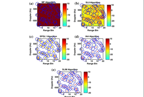
The second scenario, in which the targets do not fall onto the grid points, is more practical. In this scenario, we choose the targets randomly from all possible bins and for each target, a random number proportional to the angle resolution and a random number proportional to the Doppler resolution are added to the angle and Doppler of the target. In this case, the targets will fall off the grid points. In this simulation, we considerNt= 20 and SNR = 0 dB. Figure 6 demonstrates that the SLIM, IAA, and SPGL1 have mostly captured the targets that fall out of grid points, while the MF and SL0 have failed. Also, the SLIM algorithm has better performance compared to other ones.

In the next experiment, using Monte Carlo simula-tions, we compare the mean squared error (MSE) and peak-to-ripple ratio (PRR) of different algorithms. The MSE of target scene recovery is defined as MSE¼

X

^_−X 2

F=N; whereN=NRNAND. Also, forNttargets lo-cated at the angle-Doppler- range bins {(ki,li),i= 1,

…,Nt}, the PRR is given by

PRR¼X Nt

i¼1 X

^

ki;li

2= X^ 2_F−X

Nt

i¼1 X

^

ki;li

2

!

: ð37Þ

The results are presented based on 1000 independent tri-als. The MSEs and PRRs are respectively shown versus the

Fig. 7MSE of target scene recovery and Peak-to-Ripple Ratio (PPR) versusaanddthe number of pulses (Nt= 50, SNR = 10 dB),bandethe

number of pulses in Fig. 7a, d forNt= 50 and SNR = 10 dB, versus the number of targets in Fig. 7b, e for NP= 5 and SNR = 10 dB, and versus the SNR in Fig. 7c, f for NP= 8 and Nt= 50. By comparing the above results, one can clearly see that the SLIM algorithm achieves a lower MSE and a larger PRR in estimation of range-angle-Doppler parameters.

Also, we calculate the receiver operating characteristic (ROC) for different algorithms in order to compare their detection performance. To obtain the ROC curve, we se-lect a threshold τi. Any local maximum of the absolute value ofX that is larger thanτi will be considered as a target. The thresholdτiis then varied within an interval [τLτH] and for eachτi, the number of detected actual or false targets is recorded. By repeating 1000 trials of the experiment, we calculate the probability of detection Pd of actual targets, and the probability of false alarmPfof false targets for different values ofτias

Pd¼

the number of actual detected targets 1000Nt

ð38Þ

Pf ¼

the number of false detected targets 1000ðNRNAND−NtÞ

ð39Þ

In Fig. 8, we compare the ROC of different algorithms for NP= 8, Nt= 200, and SNR = 10 dB. As seen, in all cases the probability of detection of the SLIM is better than that of the other ones.

The running times of different algorithms are pre-sented in Table 3 for NP= 20 by averaging over 100 in-dependent trials of the experiments. We run our MATLAB 8.1 files on a PC with an Intel Core i5/ 3.4 GHz with 4 GB memory.

Obviously, in all cases, the 2D versions are much more efficient than 1D ones. Correspondingly, in Fig. 9, the run-ning times are depicted as a function ofNP. One can see

that by increasing the number of pulses, the running times of 2D algorithms remain almost constant. In other words, the computational costs of the latter algorithms are less sensitive to the number of pulses,NP. The reason is that the computational complexity of 2D SLIM does not de-pend onNPas explained in Section 4. As a result, accord-ing to Fig. 7a, d, in order to increase the performance of 2D algorithms in estimation of radar parameters, we can easily use a larger NP, while for 1D algorithms, this leads to a large increase in the running time. Moreover, it is seen from Fig. 9 that the running times of 1D algorithms are much longer than those of the 2D ones, revealing their higher computational complexities. Note that although the 2D MF has the least running time, it also generates the lowest detection and recovery performance as already depicted in Figs. 7 and 8.

6 Conclusions

We derived the 1D and 2D sparse signal models for pulse Doppler MIMO radars. The 2D SLIM algorithm was derived by direction solution of the 2D sparse model. Due to using a lower number of products in the corresponding relationships, the computational cost of 2D SLIM compared to that of the 1D one was extremely reduced. Also, simulation results showed that the 2D SLIM outperforms the other algorithms in accurate esti-mation of range, angle, and Doppler parameters.

10-4 10-3 10-2 10-1 100

Fig. 8ROC curves of different algorithms for a pulse Doppler MIMO radar

Number of Pulses (N P)

Fig. 9Comparison of running times for different algorithms

Table 3Runtime of different algorithms forNP= 20

SLIM IAA SL0 MF SPGL1

1D 74.5 264.02 456.70 5.19 147.5

2D 0.62 0.64 0.67 0.13 N/A

7 Appendix

Developing 2d CGLS

We can convert the inversing term appeared inuto a least squares (LS) form as

u¼ΦΠΦH_þηI−1_y¼BH_B−1_BH_{z ð40Þ}

The solution ofuis equivalent to minimization of the LS cost function kBu−zk2₂ with respect tou, and it can be solved using the CGLS algorithm with the following steps [36]:

<ε, whereNzis the number of elements ofz. To derive the 2D CGLS, we first presentBplas

Bp_l¼ vecðWlÞ

By incorporation of (15) and (22) in (42), we get vec(W_l) = vec(Γ⊙(AHPlΘH)) where

l+ 1 of the CGLS is demonstrated

using the Kroneker and Hadamard products properties shown in (15) and (22), andΦ=ΘT⊗Aas substituting the above results in the third and fourth steps of the CGLS and also presenting the vectorsuland rlin 2D forms asul= vec(Ul) and rl= vec(Rl), respectively, the 2D CGLS is derived as summarized in Table 2. After some mathematical manipulations using the Hadamard and Kronecker product properties, the stopping condition for the 2D CGLS is obtained by extending 1

NzkBu−zk2<εas

The authors declare that they have no competing interests.

About the authors

Mohammad Jabbarian Jahromi received the BS degree in electrical engineering from Shiraz University, Shiraz, Iran, in 2005 and the MSc degree from the Electrical and Electronic Engineering University Complex, Tehran, Iran, in 2008. He is currently working toward the PhD degree in the School of Electrical Engineering, Iran University of Science and Technology. From 2009, he was a research staff in the Signal & System Modeling laboratory, IUST. His current research interests are in the areas of array signal processing, radar signal processing, and sparse reconstruction.

Mohammad Hossein Kahaei received the BSc degree from Isfahan University of Technology, Isfahan, Iran, in 1986, the MSc degree from the University of the Ryukyus, Okinawa, Japan, in 1994, and the PhD degree in signal processing from the School of Electrical and Electronic Systems Engineering, Queensland University of Technology, Brisbane, Australia, in 1998. Since 1999, he has been with the School of Electrical Engineering, Iran University of Science and Technology, Tehran, Iran, where he is currently an Associate Professor and the head of Signal and System Modeling laboratory. His research interests include array signal processing with primary emphasis on compressed sensing, blind source separation, localization, tracking, and DOA estimation, and wireless sensor networks.

Received: 23 December 2014 Accepted: 20 July 2015

References

1. E Fishler, A Haimovich, R Blum, D Chizhik, L Cimini, R Valenzuela,MIMO Radar: An Idea Whose Time has Come. Proceedings of the IEEE Radar Conference, 2004, pp. 71–78

2. FC Robey, S Coutts, D Weikle, JC McHarg, and K Cuomo, inMIMO Radar Theory and Experimental Results. Proceedings of 38th Asilomar Conference on Signals, Systems and Computers, vol 1 (IEEE, Pacific Grove, CA, 2004), pp. 300–304

3. J Li, P Stoica, MIMO radar—diversity means superiority. Proc. 4th Adaptive Sensor Array Process Workshop. (2006). doi:10.1002/9780470391488 4. N Lehmann, F Fishler, AM Haimovich, RS Blum, D Chizhik, L Cimin, et al.

5. E Fishler, A Haimovich, R Blum, L Cimini, D Chizhik, and R Valenzuela, in

Performance of MIMO Radar Systems: Advantages of Angular Diversity. Proceedings of 38th Asilomar Conference on Signals, Systems and Computers, vol 1 (IEEE, Pacific Grove, CA, 2004), pp. 305–309

6. AD Maio, M Lops, Design principles of MIMO radar detectors. IEEE Trans. Aerosp. Electron. Syst.43(3), 886–898 (2007)

7. A Sheikhi, A Zamani, Temporal coherent adaptive target detection for multi-input multi-output radars in clutter. IET Trans. Radar Sonar Navig.

2(2), 86–96 (2008)

8. J Li, P Stoica, MIMO radar with collocated antennas: review of some recent work. IEEE Signal Process. Mag.24(5), 106_–114 (2007)

9. D W Bliss, KW Forsythe, inMultiple-Input Multiple-Output (MIMO) Radar and Imaging: Degrees of Freedom and Resolution. 37th Asilomar Conference on Signals, Systems and Computers, vol 1 (IEEE, Pacific Grove, CA, 2003), pp. 54–59

10. K Forsythe, D Bliss, G Fawcett, inMultiple-Input Multiple-Output (MIMO) Radar: Performance Issues. 38th Asilomar Conference on Signals, Systems and Computers, vol 1, (IEEE, Pacific Grove, CA, 2004), pp. 310–315 11. J Li, P Stoica, MIMO radar—diversity means superiority. The Fourteenth

Annual Workshop on Adaptive Sensor Array Processing (invited).(2006). doi:10.1002/9780470391488.

12. P Stoica, J Li, Y Xie, On probing signal design for MIMO radar. IEEE Trans. Signal Process.55(8), 4151_–4161 (2007)

13. X Luzhou, J Li, P Stoica, Target detection and parameter estimation for MIMO radar systems. IEEE Trans. Aerosp. Electron. Syst.44(3), 927–939 (2008) 14. RG Baraniuk,Compressive Sensing. IEEE Signal Processing Magazine, 2007,

pp. 118_–121

15. DL Donoho,Compressed Sensing. IEEE Transactions on Information Theory, 2006, pp. 1289–1306

16. EJ Candès, Compressive Sampling, inProc. International Congress of Mathematicians, 2006, pp. 1433–1452

17. EJ Candès, MB Wakin, An introduction to compressive sampling. IEEE Signal Process. Mag.25(2), 21–30 (2008)

18. MA Herman, T Strohmer, High-resolution radar via compressed sensing. IEEE Trans. Signal Proc.57(6), 2275–2284 (2009)

19. AP Petropulu, Y Yu, HV Poor, Distributed MIMO radar using compressive sampling. inProc,42nd Asilomar Conf, Signals, Syst, Comput., (IEEE, Pacific Grove, CA, 2008), pp. 41–44

20. T Strohmer, B Friedlander, Compressed sensing for MIMO radar—algorithms and performance. inProc. 43rd Asilomar Conf. Signals, Syst. Comput., (IEEE, Pacific Grove, CA, 2009), pp. 464–468

21. Y Yu, AP Petropulu, HV Poor, MIMO radar using compressive sampling. IEEE J. Sel. Topics Signal Process.4(1), 146_–163 (2010)

22. X Tan, W Roberts, J Li, P Stoica, Sparse learning via iterative minimization with application to MIMO radar imaging. IEEE Trans. Signal Process.

59(3), 1088_–1101 (2011)

23. A Ghaffari, M Babaie-Zadeh, C Jutten, Sparse decomposition of two dimensional signals. inIEEE International Conference on Acoustics, Speech and Signal Processing, ICASSP, (IEEE, Taipei, 2009), pp. 3157_–3160

24. A Eftekhari, M Babaie-Zadeh, C Jutten, H Moghaddam, Robust-SL0 for stable sparse representation in noisy settings. inIEEE International Conference on Acoustics, Speech and Signal Processing, ICASSP, (IEEE, Taipei, 2009), pp. 3433–3436

25. H Mohimani, M Babaie-Zadeh, C Jutten,A Fast Approach for Overcomplete Sparse Decomposition Based on Smoothed l0Norm. IEEE Transactions on

Signal Processing, 2009, pp. 289–301

26. GH Mohammadi, M Babaie-Zadeh, and C Jutten, Complex-valued sparse representation based on smoothed l0 norm. inIEEE International Conference on Acoustics, Speech and Signal Processing, ICASSP, (IEEE, Las Vegas, 2008), pp. 3881–3884

27. M Hyder, K Mahata, An improved smoothedl0approximation algorithm for

sparse representation. IEEE Trans. Signal Process.58(4), 2194–2205 (2010) 28. M Hyder, K Mahata,Range-Doppler Imaging via Sparse Representation.

Radar Conference, 2011, pp. 486–491

29. M Jabbarian-Jahromi, MH Kahaei, Two-dimensional iterative adaptive approach for a sparse matrix solution. Electron. Lett.50, 45_–47 (2014) 30. Y Yu, AP Petropulu, HV Poor,Reduced Complexity Angle-Doppler-Range

Estimation for MIMO Radar That Employs Compressive Sensing. Proc. 43nd Asilomar Conference on Signals, Systems and Computers, 2009

31. E Van Den Berg, MP Friedlander, SPGL1: a solver for large-scale sparse reconstruction. http://www.math.ucdavis.edu/~mpf/spgl1/. Accessed June 2007.

32. M Skolnik,Introduction to Radar System, 3rd edn. (McGraw-Hill, New York, 2002) 33. M Skolnik,Radar Handbook, 3rd edn. (Mc-Graw-Hill, New York, 2008) 34. KB Petersen, MS Pedersen,The Matrix Cookbook, 2008. Available:

http://www.math.uwaterloo.ca/~hwolkowi/matrixcookbook.pdf 35. T Yardibi, J Li, P Stoica, M Xue, AB Baggeroer, Source localization and

sensing: a nonparametric iterative adaptive approach based on weighted least squares. IEEE Trans. Aerosp. Electron. Syst.46, 425–443 (2010) 36. R Aster, B Borchers, C Thurber,Parameter Estimation and Inverse Problem

(Elsevier Academic, Burlington, MA, 2005)

37. AN Langville, WJ Stewart,The Kronecker Product and Stochastic Automata Networks. Elsevier Journal of computational and Applied Mathematics, 2004, pp. 429–447

38. G Wu, Z Zhang, E Chang,Kronecker Factorization for Speeding up Kernel Machines. SIAM International Conference on Data Mining, 2005, pp. 611–615 39. H He, P Stoica, J Li, Designing unimodular sequence sets with good

correlations—including an application to MIMO radar. IEEE Trans. Signal Process.57, 4391–4405 (2009)

Submit your manuscript to a

journal and benefi t from:

7Convenient online submission

7Rigorous peer review

7Immediate publication on acceptance

7Open access: articles freely available online 7High visibility within the fi eld

7Retaining the copyright to your article