Exploiting Acoustic Similarity of Propagating
Paths for Audio Signal Separation
Bin Yin
Faculty of Electrical Engineering, Eindhoven University of Technology, P.O. Box 513, 5600 MB Eindhoven, The Netherlands Storage Signal Processing Group, Philips Research Laboratories, P.O. Box WY-31, 5656 AA Eindhoven, The Netherlands Email:[email protected]
Piet C. W. Sommen
Faculty of Electrical Engineering, Eindhoven University of Technology, P.O. Box 513, 5600 MB Eindhoven, The Netherlands Email:[email protected]
Peiyu He
Faculty of Electrical Engineering, Eindhoven University of Technology, P.O. Box 513, 5600 MB Eindhoven, The Netherlands University of Sichuan, Chengdu 610064, China
Email:[email protected]
Received 20 September 2002 and in revised form 26 May 2003
Blind signal separation can easily find its position in audio applications where mutually independent sources need to be separated from their microphone mixtures while both room acoustics and sources are unknown. However, the conventional separation algorithms can hardly be implemented in real time due to the high computational complexity. The computational load is mainly caused by either direct or indirect estimation of thousands of acoustic parameters. Aiming at the complexity reduction, in this paper, the acoustic paths are investigated through an acoustic similarity index (ASI). Then a new mixing model is proposed. With closely spaced microphones (5–10 cm apart), the model relieves the computational load of the separation algorithm by reducing the number and length of the filters to be adjusted. To cope with real situations, a blind audio signal separation algorithm (BLASS) is developed on the proposed model. BLASS only uses the second-order statistics (SOS) and performs efficiently in frequency domain.
Keywords and phrases:blind signal separation, acoustic similarity, noncausality.
1. INTRODUCTION
In recent years, blind signal separation (BSS) has grasped the attention of lots of researchers because of its numer-ous attractive applications in speech processing, digital com-munications, medical science, and so on. BSS, within the
framework of independent component analysis (ICA) [1,2],
deals with the problem of separating statistically indepen-dent sources only from their observed mixtures while both the mixing process and source signals are unknown.
For acoustical applications, it can be used to extract indi-vidual audio sources from multiple microphone signals when several sources are simultaneously active [3]. In other words, it becomes possible, for instance, in a teleconferencing sys-tem, to pick up one desired speech signal under a relatively low signal-to-noise ratio (SNR) (so called “cocktail party ef-fect”).
For a certain combination of source-sensor positions, instead of solving three-dimensional wave equations, the
acoustic transmission from the source to the sensor can be simply described using an impulse response, which is ob-tained by measuring the signal received by the sensor after a sound pulse has been emitted from the source. An example
is shown inFigure 1.
Thus, an acoustic mixing process in a reverberant envi-ronment can be modelled as
x[k]=(h∗s)[k], (1)
wheres[k]=(s1[k], . . . , sn[k])Tandx[k]=(x1[k], . . . , xn[k])T
denote the vectors of audio sources and microphone signals, respectively, and
h[k]=
h11[k] h12[k] · · · h1n[k]
..
. ... . .. ...
hn1[k] hn2[k] · · · hnn[k]
is a transfer function matrix whose elementhi jexpresses the
room impulse response (RIR) from the jth source to theith
microphone,kis the discrete-time index which corresponds
to the sampling moment,∗denotes linear convolution and
( )T denotes matrix transpose. Here we assume the numbers
of sources and microphones are the same and the environ-ment is noise free.
The sources can be separated either by inverting the
transfer function matrixh[k] after having obtained the
es-timate of the individualhi j(known as forward model
meth-ods), or by directly finding a demixing matrixG[k] which
satisfies (G∗h)[k]=I[k]P, whereI[k] is a diagonal
trans-fer function matrix andPdenotes a matrix of permutation
(known as backward model methods).
In principle, a sound pulse emitted from the source will be reflected infinite times by the walls and other obstacles, so an IIR filter seems to be suitable to describe the
characteris-tics of an RIR. However, as shown inFigure 1, an RIR reveals
a decaying waveform so that after a certain number of taps the residual signal becomes too weak to be detected by the sensor (e.g., human ears). Therefore, in practice, an FIR fil-ter can be a quite acceptable approximation. In audio separa-tion and many other applicasepara-tions, an FIR filter, for instance, having 1000–2000 taps with 8 kHz sampling frequency in a
usual office, gives a good performance. An FIR filter is
pre-ferred because it provides much convenience when applied in digital signal processing.
For RIRs of such a considerably long length, in both for-ward and backfor-ward model methods, audio separation be-comes a huge task due to the estimation of thousands of
co-efficients. It gets even more challenging in real-time
imple-mentations which are often needed in audio signal process-ing.
In this paper, aimed at the feasibility of real-time appli-cations, a simplified mixing model is proposed which takes advantage of acoustic propagation similarities. In literature, a model which is close to the proposed one has also been used
in signal separation analysis, especially in 2×2 case, for
exam-ple, in [4,5,6]. By only considering the antidiagonal terms
in the mixing matrix, the theoretical analysis of BSS became much more simplified. However, its feasibility has never been explicitly studied from an application point of view. In [4], two possibilities were given. One was that, two sources were standing near their own sensors so that only the transfer functions in two coupling paths (antidiagonal terms in the mixing matrix) should be taken into account; the other was that, in an anechoic, isotropic, and homogeneous environ-ment, a coupling path could spatially equal the direct path in cascade with an auxiliary path. The latter resembles the form of the proposed model in this paper. In general, these two hy-potheses will not hold in a natural reverberant environment. Besides, the noncausality introduced during the simplifica-tion has not been considered, which is inevitable according
to the analysis in Section 4. Another paper that should be
mentioned is [7], where the authors used a compact (1 cm)
microphone array in order to describe the difference between
the acoustical paths with a pure time delay. The signal sepa-ration was done in two stages: first sepasepa-ration by estimating
1.5
Figure1: An example of an impulse response between two points in a room.
and inverting the delay matrix and further separation with a feedback network. The idea is somewhat related, but we replace the pure delay with a filter of which the characteris-tics will be carefully studied. The proposed model provides the possibility of achieving signal separation in one step and relieving the excessive constraints on the dimension of the microphone array. On the basis of the new model, a BSS al-gorithm is described which only uses second-order statistics
(SOS) and is efficiently realized in frequency domain. By
ap-plying the simplified mixing model, it is shown that the num-ber of filters to be estimated is reduced to some extent. Be-sides, the taps of filters are significantly decreased in the case where microphones are intentionally closely placed. Several other advantages are mentioned as well. As a whole, they ef-fectively give a possibility to a real-time implementation of audio source separation.
The remainder of this paper is organized as follows. In Section 2, concentrating on a 1-speaker-2-microphones system, we study the similarity between acoustic paths by
defining an acoustic similarity index (ASI).Section 3gives a
simplified mixing model for blind audio source separation
in both time and frequency domain. In Section 4, a
non-blind speech signal separation scheme is designed in order to demonstrate the feasibility of the proposed model. To be able to cope with a real audio signal separation problem, we develop an adaptive BSS algorithm for the new mixing model inSection 5. Finally,Section 6gives the conclusions.
2. SIMILARITY OF ACOUSTIC PATHS 2.1. Room impulse responses
An RIR describes the characteristics of a propagating path when a sound propagates from its source to a sensor (say
a microphone). The bandwidth needed for an RIR differs
according to a specific application. For voiced speech, the upper bound drops below 4 kHz. Therefore, in speech
sig-nal separation, a sampling frequency fsof 8 kHz is adequate.
Without extra indication, fs = 8 kHz will be used in this
Throughout the whole paper except for the experiments on the recorded real-world data, we employ a Matlab pro-gram “Room” [8], which applies the image theory [9], to generate RIRs. This choice is made for several reasons.
(1) The experimental environment is clean and we are able to have accurate control over the experimental con-ditions, such as the room dimensions, wall reflection
coefficients, and, especially, the subtle changes of the
source and microphone positions.
(2) The image solution of a rectangular enclosure, like
the office environment, rapidly approaches an exact
solution of the wave equation as the walls of the room become rigid. Under typical conditions, the
fre-quency range of 100 Hz–4 kHz, wall reflection coeffi
-cients greater than 0.7, and both source and micro-phone not close to the wall, it does not introduce se-rious problems into the final result [9].
Now let us have a close look at the characteristics of an
RIR. The room dimensions are uniformly adopted as 4 m×
5 m×3 m (width×depth×height), like that of a normal office.
Placing one of the ground corners at the origin of a three-dimensional coordinate system, we can express any location
in the room with a triplet (x, y, z), withx,y, andzthe width,
depth, and height, respectively. By default, the sources and
microphones are located at the plane ofz=1.5 m.
Listed in Figure 2are two RIRs with different wall
re-flections, corresponding to an almost anechoic environment
with a reverberation timeT60=0.116 second and a strongly
reverberant environment withT60 = 0.562 second. The
re-verberation timeT60 is defined as the time needed for the
sound pressure level to decay by 60 dB when a steady-state
sound source in the room is suddenly switched off[10]. The
first observation is that the RIR with T60 = 0.562 second
has much denser reflections and much longer decaying time
than that with T60 = 0.116 second. The second is that
the RIR with T60 = 0.562 second becomes nonminimum
phase. Usually a nonminimum phase RIR occurs when a microphone picks up an echo stronger than the direct sig-nal. This can happen in a strongly reverberant environ-ment, as shown in this case, and also when a microphone is placed more closely to a wall or other obstacles than to the source.
2.2. Susceptibility of a room impulse response
Due to the wide range of wavelengths (from about 17 mm to 17 m) and the low propagating speed of a sound, a slight change of the source or sensor position may influence the fine structure of the impulse response significantly.
To study this susceptibility, consider a 1-speaker-2-microphone setup in the aforementioned room. The RIRs
from the speaker at (xs, ys, zs) to the microphone 1 at
The DRIR is used to describe the variation of the RIR
when the microphone position is shifted from (x1, y1, z1) to
For convenience of later analysis and processing, we like to express it in the form of an FIR filter. We understand from Section 2.1that an RIR could lose the minimum phase char-acteristic in certain acoustical conditions. So, without any
prior knowledge, we have to assumeh11[k] a nonminimum
phase FIR filter. The impulse response of its stable inver-sion will be a noncausal infinite double-sided converging
se-quence. After the convolution in (4),∆h21[k] also becomes a
noncausal double-sided IIR filter. The exception arises only
when the zeros ofh11[k] outside the unit circle are cancelled
by those ofh21[k], which is unlikely to happen in reality. To
make it suitable for practical use, we execute two operations:
first shift it by a delay ofτsamples, and then truncate it such
that
∆h˜
21[k]=Trc h21∗h−111
[k−τ], (5)
where Trc{·}denotes the truncation that cuts offall the taps
before k = 0 and after k ≥ L. The relationship between
∆h˜21[k] and∆h21[k] can be written as
21[k] denotes an error filter varying with different choices of
τ andL, obviously21→0 withτ, L→ ∞. Convolving both
negligible for certain applications, (7) can be simplified as
h21[k−τ]≈
of expression. Therefore, from now on, ∆h21[k] denotes a
causal FIR filter of length L. To distinguish, we denote the
IIR∆h21[k−τ] in (6) as∆ho21[k].
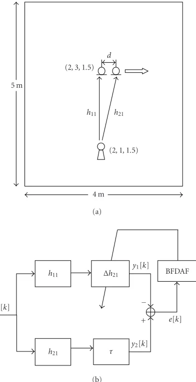
In the following simulation, we study the feasibility of the above expression in various acoustical situations. Depicted in Figure 3a is the simulation setup, where the source and
one microphone stand still to fix h11 and the other
micro-phone moves along the hollow arrow to give varioush21’s.
We use the efficient block frequency domain adaptive
filter-ing (BFDAF) algorithm for the DRIR estimation. The block
diagram of the estimation scheme is plotted inFigure 3b. The
input signals[k] is white and the delay adopted is always half
the filter length, that is, τ = L/2. The simulation is done
with T60 = 0.116 second,0.270 second, and 0.562 second,
1
0.5
0
Am
p
li
tu
d
e
0 0.02 0.04 0.06
Time (s) (a)
1
0.5
0
Am
p
li
tu
d
e
0 0.1 0.2
Time (s) (b)
1
0
−1
Im
ag
e
−1 0 1
Real (c)
1
0
−1
Im
ag
e
−1 0 1
Real (d)
1
0.9
0.8
Im
ag
e
−0.5 0 0.5 Real
(e)
1
0.9
0.8
Im
ag
e
−0.5 0 0.5 Real
(f)
Figure2: Comparison of zero distributions. Left column (T60=0.116 second): (a) RIR, (c) zero distribution at thezplane, (e) zooming in
the area with broken lines in (c). Right column (T60=0.562 second): (b) RIR, (d) zero distribution at thezplane, (f) zooming in the area
5 m
(2,3,1.5) d
h11 h21
(2,1,1.5)
4 m (a)
s[k]
h11 ∆h21
y1[k]
BFDAF
−
+ e[k]
h21 τ
y2[k]
(b)
Figure 3: The acquisition of the DRIR∆h21: (a) the simulation
setup in the room, (b) the block diagram of the acquisition scheme.
Figure 4a, where the mean square error (MSE) at the vertical axis is defined as
MSE=lim
k→∞10 log
T
l=−Te[k+l] 2
T
l=−Ty2[k+l] 2,
e[k+l]=y2[k+l]−y1[k+l],
(9)
whereTdenotes a certain number of samples chosen for
av-eraging. The corresponding h11’s are also plotted inFigure
4b. In fact, the residual signale[k] in (9) satisfies
e[k]=R 21∗s
[k], (10)
which reflects the normalized modelling error when we
ex-pressh21ash11convolved with an FIR∆h21.
For a given filter lengthL, two facts can be observed.
First, the more reverberant the environment is, the more modelling error exists. This phenomenon may be intuitively
−10 −15 −20 −25 −30 −35 −40 −45 −50
MSE
(dB)
0 10 20 30 40 50 60 70 80 90 100
d(cm) L=2048
L=2048
L=2048
Weak reverberation Mild reverberation Strong reverberation
(a) 1
0.5 0
0 0.05 0.1 0.15 0.2 0.25 0.3 T60=0.116 s
1 0.5 0
0 0.05 0.1 0.15 0.2 0.25 0.3 T60=0.270 s
1 0.5 0
0 0.05 0.1 0.15 0.2 0.25 0.3 T60=0.562 s
Time (s) (b)
Figure4: The feasibility study of the expression in (8). (a) Magni-tude of the residual signals. (b) RIRs in the three acoustical condi-tions.
explained as follows. With the increase of reverberation, the RIR gets longer; besides, its inverse becomes double sided and both tails take quite some time to converge due to the fact that its zeros tend to distribute more closely to the unit circle, and even exceed it in the case of a large reverberation. This
can be seen inFigure 2d. Thus, truncating in (5) introduces
more errors. Secondly, the further the two microphones are placed away from each other, the more modelling error we have. This trend happens rapidly, especially when the micro-phone spacing increases from 1 cm to 20 cm. We will analyze
For practical applications, one cares mostly not about the existence of this error, but how small it should be so as to provide a satisfactory result to a specific application. In au-dio signal separation, despite a certain modelling error intro-duced when the expression (8) takes place, the separation can still be achieved in the sense that the cross talk left is inaudi-ble or not disturbing any more to human ears. Therefore, by
defining a DRIR∆h21, we have effectively related the RIRh21
toh11.
2.3. Acoustic similarity index
The second fact above suggests that as two microphones get closer, a similarity may start to play a role between the two acoustic paths, despite the susceptibility of an RIR. It sim-plifies the description of the DRIR and in turn decreases the modelling error in (7). These two aspects are not conflicting
because whether the similarity or difference prevails depends
on the accuracy of our interest. Let us have a closer look at
several DRIRs withT60 = 0.270 second obtained in the last
simulation, which is considered to be a normal situation.
Withd = 1 cm, the DRIR appears like a pure time
de-lay (Figure 5a), and accordingly, its amplitude frequency re-sponse looks quite flat in the most part of the spectrum and really fluctuate only at a limited number of high frequency components (Figure 5b). When the spacing increases, be-sides the central tap, more taps start to grow in magnitude so
that more frequency components get influenced (Figures5c,
5d,5e, and5f). This is understandable because asdincreases the low frequency components of a sound signal see
propa-gating path difference later and less than the high frequency
components due to their longer wavelengths. The simulation implies that in general the characteristics of RIRs are not very much influenced by a small shift (within 5 cm in this case) of the objects because the wavelengths of the audio sig-nals (greater than 9 cm for voiced speech) are well above this scale. The two acoustical paths before and after the shift can be regarded to be alike up to a time delay.
Now we are in the position of defining an ASI that
re-flects the degree of this similarity. We put the coefficients of
∆h21[k] in a vectorc=[c1, . . . , cL]T. The ASI can be defined
whereEmrepresents a matrix with one at the m-mth
posi-tion and zeros elsewhere, andEmc=[0, . . . , cm, . . . ,0]Twhere
m = arg maxi{|ci|}. The exponential part expresses the
ra-tio between the power of the central tap and the sum of the powers of the rest, which, in frequency domain, can be inter-preted as the flatness of the spectrum. The nonlinear
func-tion exp{·}is adopted in order to reflect the rapid drop of the
ASI as soon as the DRIR starts to differ from a pure time
de-lay. We calculate the corresponding ASI values for the DRIRs
obtained in the last subsection and record them inFigure 6a.
For all situations, the general trend is the same: the ASI
decreases as the microphone spacingdincreases. Whend
ap-proaches zero, the ASI apap-proaches one, the highest value of
the similarity. It can be obtained from (11) with∆h21a
sin-gle pulse in that case. In an almost anechoic environment,
the ASI keeps very close to one even withdlarge up to 20 cm
(solid line). It is because any RIR resembles a single-pulse-like form due to very few reflections, so that any two RIRs can be similar regardless of the object positions. While in more reverberant cases the ASI declines drastically at the first several centimeters (dashed and dotted lines), and after that it stays almost zero, meaning that the similarity between the two acoustic paths has gone.
Through the following analysis, we can see a bit more how the ASI varies according to the shape of an RIR. Suppose
we have two RIRs, each of two taps, and they are written inz
domain as
The first term is the so-called central tap. Since the rest of the taps converge in magnitude, the next couple of terms be-come very critical for determining the ASI. If the microphone
spacingdis so small thatg2=g1holds, then we have
The values of the side taps are reduced because of the
sub-traction (r2−r1). Whenr1andr2are comparable, meaning
that the two RIRs are quite similar, the reduction could be very significant. This will lead to a high ASI value. Other-wise, it will be very much likely to get a low ASI except that
the values ofri(i =1,2) themselves are much smaller than
one, for instance, in the case of a very weak reverberation. This rough analysis is basically also applicable to the practi-cal situations although the expression gets more complicated because of the longer RIRs.
Hence, in order to get a higher ASI value, we have to ei-ther let the environment less reverberant or make the
mi-crophones more closely spaced. These two effects can be
ob-served inFigure 6a.
Naturally, the fact that with a small microphone spac-ing a DRIR looks sspac-ingle-pulse like provides a possibility to
use less filter taps. We repeat the simulation inFigure 4with
T60=0.270 second and variousL’s. The results are plotted in
Figure 6b. Three microphone spacings are chosen. Ford =
0.5 cm, the modelling error stays below −18 dB even with
1
0.5
0
−0.5
0 500 1000 1500 2000 2500
Filter taps (sample)
A
m
plitude
(a)
10 0 −10 −20 −30
Po
w
er
(d
B
)
0 1 2 3 4
Frequency (kHz) (b)
1
0.5
0
−0.5
0 500 1000 1500 2000 2500
Filter taps (sample)
Am
p
li
tu
d
e
(c)
10 0 −10 −20 −30
P
o
w
er
(dB)
0 1 2 3 4
Frequency (kHz) (d)
1
0.5
0
−0.5
0 500 1000 1500 2000 2500
Filter taps (sample)
Am
p
li
tu
d
e
(e)
10 0 −10 −20 −30
P
o
w
er
(dB)
0 1 2 3 4
Frequency (kHz) (f)
Figure5: The DRIRs for different microphone spacingdwithT60 =0.270 second. Left column: impulse responses in time domain, (a)
d=1 cm, (c)d=5 cm, (e)d=20 cm. Right column: corresponding amplitude responses in frequency domain, (b)d=1 cm, (d)d=5 cm, (f)d=20 cm.
so much that most of side taps can be practically neglected. The ASI equals 0.89, reflecting the high similarity of the two
RIRs. Ford=2 cm, the MSE needsL >750 to remain below
−20 dB since the tail of the DRIR includes stronger taps and,
when truncated, significant errors will occur.
Correspond-ingly, the ASI decreases to 0.58. Ford = 10 cm, the ASI is
0.03, meaning actually that no similarity exists. The conclu-sion is that for a certain MSE requirement, fewer taps are needed with a smaller microphone spacing.
We must point out that the simulation results indicate
some general rules, but these concrete numbers can
fluctu-ate in different acoustical environments. For instance, for the
same microphone spacingd, the ASI value can be different
with the variation of the distancewfrom source to
micro-phone. In the former simulations, thewwas set around 2 m.
Here we change the wto see how the ASI changes
accord-ingly. The results are obtained withT60=0.270 second and
plotted inFigure 7.
When thewis smaller than 1 m, the ASI becomes above
1
0.8
0.6
0.4
0.2
0
ASI
0 2 4 6 8 10 12 14 16 18 20
Microphone spacingd(cm) Weak reverberation
Mild reverberation Strong reverberation
(a)
−5
−10
−15
−20
−25
−30
−35
MSE
(dB)
0 500 1000 1500 2000 2500
Filter taps (sample) d=0.5 cm
d=2 cm d=10 cm
(b)
Figure6: (a) The ASI versus the microphone spacingdin different
acoustic situations (L=2048). (b) The modelling error versus the length of the DRIR withT60 = 0.270 second (2048 taps used for
the RIRs). The source-to-microphone distancewequals 2 m in both figures.
ASI=0.03 withw=2 m), meaning that the similarity starts
to play a role. The reason is that when the microphones move to the source, the RIRs tend to be minimum phase because
the distance w is small compared to that from the
micro-phones to the walls so that the direct sound is more likely to
1 0.8 0.6 0.4 0.2 0
ASI
50 100 150 200 250 300
Microphone-source distancew(cm) ASI (d=5 cm)
ASI (d=10 cm)
MSE (d=5 cm) MSE (d=10 cm)
−10
−15
−20
−25
−30
−35
MSE
(dB)
Figure7: The ASI and MSE versus the source-to-microphone dis-tancewin different microphone spacings.
be dominant over the reflections. This leads to shorter RIRs as well as their inverses. Consequently, the ASI becomes high. This provides us with another possibility to acquire a high ASI value. An interesting phenomenon can be observed that,
ford=5 cm, the ASI begins to increase at a low level when
wis larger than 2 m. It can be explained by the effect that a
certain microphone spacing becomes relatively small if the microphones move away from the source, resulting in an
in-crease of the ASI. This effect is always there, but until thew
gets large enough, it does not prevail over the other
oppo-site effect that ASI decreases due to the nonminimum phase
tendency of RIRs.
In general, the simulation results indicate that one should expect a more single-pulse-like DRIR within 5–10 cm mi-crophone spacing under the normal room acoustics, corre-sponding to an ASI value above 0.5.
3. A SIMPLIFIED MIXING MODEL
In the case of a high ASI, introducing a simplified mixing model becomes very attractive to audio signal separation
which usually suffers from high complexity. To derive the
new model, we first generalize the relationship in (8) to the
case ofnsources andnmicrophones
hml[k−τ]=∆hml∗hll[k], m, l=1, . . . , n, m=l,
(15)
where the modelling error is omitted. Then we can rewrite the model in (1) as
x[k−τ]=∆h∗s[k], (16)
wherex[k−τ]=(x1[k−τ], . . . , xn[k−τ])T,s[k]=((h11∗
s1)[k], . . . ,(hnn∗sn)[k])T, and
∆h[k]=
δτ[k] ∆h12[k] · · · ∆h1n[k]
..
. ... . .. ...
∆hn1[k] ∆hn2[k] · · · δτ[k]
For convenience of the latter expression,δ[k−τ] is written
asδτ[k] representing a time delay ofτsamples. Since the
mi-crophones should be closely spaced relative to each source, a microphone array will be a reasonable solution. The
compo-nents in the vectorsare mutually independent due to the
as-sumed independence between the sources, so the signal sep-aration can be achieved after obtaining the estimation of the
mixing matrix∆h[k].
Using this simplified model in audio signal separation has several specific advantages.
(1) What we attempt to recover are the signals propagating and arriving just in front of the microphones before mixing, that is, the sources convolved by the RIRs from their emitting points to the respective microphones, which often sound more natural than the clean sources themselves when there is not too much reverberation present.
(2) The number of filters to be estimated is reduced from
n2ton(n−1).
(3) Furthermore, with the existence of the similarity
be-tween acoustic paths, fewer coefficients are required to
describe∆hml’s because they appear very much like a
single-pulse function. As a result, the computational load for the mixing model estimation can be signifi-cantly reduced.
As seen in (16), in a reverberant environment, micro-phone signals are convolutive mixtures of original sources.
For much more efficient implementation, we will transform
the problem into the frequency domain so as to realize signal separation simultaneously for every frequency component as
in the case of an instantaneous mixing [11,12].
The discrete Fourier transform (DFT) allows us to ex-press circular convolutions as products in frequency domain, while in (16) linear convolutions are assumed. A linear con-volution can be approximated by a circular concon-volution if
L N, whereN denotes the number of points within one
data frame in the DFT. Also a linear time shifting in∆hcan
be approximated by a circular time shifting ifτN.
There-fore, we can write approximately
Xωi, p−τ≈∆ᏴωiSωi, p,
ωi=(i−1)
N 2π, i=1, . . . , N,
(18)
whereωidenotes theith frequency component;
X(ωi, p−τ)=(X1(ωi, p−τ), . . . , Xn(ωi, p−τ))T (19)
represents the DFT of the microphone signals where
Xm(ωi, p−τ) comes from the DFT of the vector of signals
from themth microphone, that is,
xm[p−τ]=
the frequency domain counterpart of the filter matrix∆h[k]
and can be expressed as
∆Ᏼωi=
4. SIGNAL SEPARATION IN THE2×2CASE
In this section, we take a 2-speaker-2-microphone system as an example to demonstrate the feasibility of the proposed mixing model in speech signal separation.
A simulation scheme of the separation is shown in Figure 8. The left diagram expresses the parameter measur-ing part where two BFDAF algorithms are used in parallel,
and the right describes the separation part. TheΛ−1[k] acts
as a postprocessing filter that is the inversion of
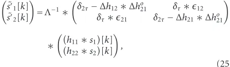
Λ[k]=δ2τ−∆h21∗∆h12
[k], (23)
where∆hi j must be measured when onlysj is active, so the
measurement may be first done with two sources made alter-natively active, and after convergence of the filter parameters, the separation is then switched on. If we rewrite the mixing process in (16) without the modelling error as
ml∗hll)[k] accurately hold, after the demixing
inFigure 8, we have
elling error as defined in (6). When the modelling errors are
zero, the separation part inFigure 8functions exactly as an
inversion of the mixing process and a perfect signal separa-tion will be achieved. The cross talk left depends on the mag-nitude of nonzero modelling errors.
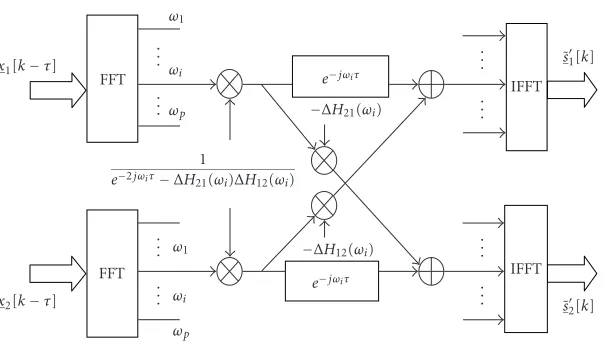
The separation may be implemented efficiently in
fre-quency domain as well. Its corresponding frefre-quency domain
structure is given inFigure 9, where the inputxito the FFT
S1
Figure8: The signal separation scheme (2×2 case).
x1[k−τ]
Figure9: The separation implemented in frequency domain (2×2 case).
by bufferingNconsecutive data samples. The operations
be-tween FFT and IFFT blocks equal the inversion of the mix-ing matrix in frequency domain given in (18). One can see that the separation is independently operated for each
fre-quency componentωi, which converts the convolutively
mix-ing problem into an instantaneous one.
As mentioned inSection 2.1, the time delayτ is
intro-duced for the causal stable inversion of a nonminimum phase
RIR. In general one can simply let τ = L/2, but it is not
necessarily like that. The proper choice of τ relies on
sev-eral factors, for instance, the wall reflection and the distance between sources and microphones. In particular, if the re-verberation is quite weak and the audio source is located close to its microphone (say within several 10 centimeters),
τ may be chosen as zero since in this case RIRs are normally
minimum phase. The advantage is that less taps are needed or with the same taps one can provide the right tail with more freedom, which probably gives more significant infor-mation. The detailed experimental results can be found in [13].
As for the postprocessing filterΛ−1, it again concerns the
inversion of a nonminimum phase filter. To solve the prob-lem, one possibility is simply moving it away
(correspond-ingly omitting the term 1/(e−2jωiτ−∆H
12(ωi)∆H21(ωi)) in
Figure 9) because it has nothing to do with the effectiveness of the separation; the other possibility is keeping it there to improve the sound quality at the cost of introducing another extra time delay.
In order to evaluate the separation result with respect to
different filter lengthsL’s under different ASI values, we
de-fine the following separation index (SI):
SIm=lim
andTis a proper time period. If a white noise is assumed as
4 m
5 m
d
2 m
S1(1.5,1,1.5) S2(2.5,1,1.5)
Filter taps (sample)
SI
(dB)
(a)
60 50 40 30 20 10
SI
(dB)
500 1000 1500 2000
d=0.5 cm d=5 cm d=10 cm
Filter taps (sample)
(b)
Figure10: The SI versus the number of taps for DRIR. (a) The sim-ulation environment (T60=0.27 second). (b) The results in three
different microphone spacings.
inzdomain as
SIi=10 log
Λ−1z−1z−2τ−∆hmlz−1∆ho lm
z−1]
×hmmz−12dz
× Λ−1z−1z−τlmz−1hmmz−12dz
−1 .
(28)
In the current case where the sources are known to be alternatively active, one is able to get the DRIRs with only one source present, which makes the separation nonblind, so the SI value in fact indicates the maximum separation ef-fect one can achieve when using the simplified mixing model
with some givenLandτ. In real BSS, extra modelling errors
will exist due to nonoptimal estimation of DRIRs. Thus the SI will no longer reach its maximum. By definition, the SI is equivalent to an SNR or an SIR (signal-to-interference ratio) normally used in literature.
The simulation is done as described inFigure 10a. The
reverberation time in the room is set as T60 = 0.27 second
and input signals are white noise sampled in the frequency
of 8 kHz. The results are plotted inFigure 10b. For a better
comparison, the highest SI values of the three microphone spacings are normalized to be the same. In all cases, the SI de-creases with the reduction of the filter taps, which coincides very well with (28). For the same filter length, the SI with
d =0.5 cm is higher than that withd =5 cm by more than
5 dB. That is because the DRIR in the former case resembles a single pulse due to the high similarity of the acoustical paths
(ASI = 0.85). It makes possible a considerable filter length
reduction. The SI withd= 10 cm is about 3 dB lower than
that withd=5 cm, meaning that the acoustic similarity
dis-appears further.
Two conclusions can be drawn. First, thanks to the sim-ilarity between the acoustical paths, the computational load of the audio signal separation can be significantly relieved,
while the separation effect stays still reasonably good (above
20 dB). This gives us an opportunity to implement an au-dio signal separation in real time. Secondly, with large micro-phone spacings, a satisfying separation can be still acquired if the DRIRs are provided with enough taps. Hence, the pro-posed mixing model is also suitable for a normal use where microphones are not closely spaced, having the advantage of less filters to estimate.
Notice that the proposed model remains feasible as long
as the difference between acoustical paths is distinguishable.
A too small microphone spacing (d <1 cm) gives little path
difference to low frequency components of sources. A higher
accuracy (more bits in digital signal processing) during sam-pling helps, but will be limited by the background noise level.
The small path difference can accumulate after a number
of reflections, so it reveals itself strongly in the reverbera-tion part. However, since the signal power decays
exponen-tially, the path difference becomes “invisible” especially at
the presence of noise. Obviously, the separation fails when
microphones are placed at the same point since no diff
er-ence can be detected regardless of the given accuracy. In the
case of a large spacing (d > 10 cm), the time delay of the
arrival of the direct sound can help to “build” a path diff
er-ence to avoid the spatial aliasing of high frequency compo-nents.
5. ADAPTIVE BLIND SIGNAL SEPARATION ALGORITHM
In literature, to achieve BSS, a variety of approaches based
on different methodologies and theories have been proposed,
which in general fall into two categories. If sources are sta-tionary, Gaussian processes, it can be shown that blind sepa-ration is impossible in a certain sense. By stipulating non-Gaussianity on source signals, one can apply higher-order statistics (HOS) evaluation to realize separation. The meth-ods in the first category are characterized by computing HOS
explicitly [14,15,16,17], or implicitly [18,19], ML [20],
IN-FOMAX [21], MMI [22], and NM [23] to achieve separa-tion. While in the other category, with the help of some extra
constraints, SOS is proved to be sufficient to determine the
mixing process, for instance, additional time-delayed
corre-lations [24], sources of different spectra [15,25,26], spectral
matching and FIR constraints on mixing process [27], and nonstationary sources [28].
In this paper, by taking advantage of the nonstationarity of the audio sources, we develop an adaptive blind audio sig-nal separation (BLASS) algorithm in frequency domain only based on SOS evaluation. Apparently, from the application point of view, an SOS method is preferred due to its less com-putational complexity and stronger robustness to noise.
Some first theoretical proof of how the BSS problem of nonstationary sources can be solved only using SOS has been given in [28]. We are not going to look at that further be-cause it is out of the scope of this paper. Roughly speaking, the point is on the fact that, with the help of nonstationarity, one is able to do decorrelation through time to eliminate the ambiguity of the mixing (or demixing) model.
5.1. A gradient descent rule
Recalling the proposed mixing model in frequency domain
from (18), after having obtained the mixing matrix∆Ᏼ(ωi),
the separated signals for each frequency component can be written as
Sωi, p=∆Ᏼ−1ωiXωi, p−τ,
ωi=(i−1)
N 2π, i=1, . . . , N.
(29)
We construct an objective function as follows:
J(p)=
of a matrix and the inversion of the resulting matrix,
respec-tively,Rx(ωi, p−τ) andRs(ωi, p) represent the power matrix
ofXandSfor each frequency component. Basically they are
the function of a differentpbecause of the nonstationarity of
audio signals. The objective function is in fact the sum of off
-diagonal elements in the power matrix of the signal vectorS
over all the frequency components, reflecting the cross power spectra between the demixed signals. Due to the mutual
in-dependency of the sources,J(p) should reach its minimum.
Therefore, the mixing matrix may be learned by means of a gradient descent algorithm
notes the complex conjugate of a matrix, andµis a positive
factor that determines the rate of updating. The gradients in (32) are given by
∂J(p)
∂∆Ᏼωi
=−2 ∆Ᏼ−HωiRsωi, p−diag Rsωi, p Rsωi, p∗,
(33)
Rsωi, p=∆Ᏼ−1ωiRxωi, p∆Ᏼ−Hωi, (34)
where diag{·}denotes taking the diagonal elements of a
ma-trix and putting them at the corresponding positions of a zero matrix.
5.2. Constraints on the gradients
There are two constraints on the gradients during parame-ter updating. The diagonal elements in each gradient matrix
∂J(p)/∂∆Ᏼ(ωi) must be zero because the parameters have
Secondly, the gradients have to be constrained in order to
make the time domain solutions satisfying∆h[k]=0 fork >
L. This is important for the expression in (18) to have a good
approximation. Thus we use the following constraint [29]:
Z is anN×N diagonal matrix withZii = 1 fori ≤Land
Zii = 0 fori > L,F denotes the Fourier matrix operating
DFT, and accordinglyF−1operates IDFT.
As well known, the side effect of the frequency domain
separation is that one cannot guarantee that the frequency components used to reconstruct the time domain output come from the same source because any permutation of the coordinates at every frequency will lead to exactly the same
J(p). If the permutation appears, generally the spectra of the
estimated filters will become nonsmooth. Forcing zero
coef-ficients fork > Lin time domain equivalently smooths their
spectra through a convolution with a sinc function in fre-quency domain. Therefore, the permutation problem can be
effectively removed by applying the constraintᏯ(2).
In addition, there is another point which may have not been realized in previous literature. If one of the sources does
not have any power at a certain frequency component ωi,
the separation fails because∆Ᏼ(ωi) is singular and therefore
∆Ᏼ−1(ωi) does not exist. The smoothing of the spectrum by
Ꮿ(2)helps to remove the zeros so as to relieve the problem to
some extent.
5.3. Practical approximation
Although in general audio signals are nonstationary, it is still said that human voice has temporally stationary structure within a few 10 milliseconds [30]. This means it is possible to use time averaging to approximate the SOS needed in our algorithm:
Rxωi, p≈ 1
2T
T
q=−T
Xωi, p+qXHωi, p+q, (38)
whereTis properly chosen to make the averaging within the
stationary period. Formula (38) is only needed for the ini-tialization of the power matrices. During the adaptation the power estimates are updated using
Rxωi, p+ 1=αRxωi, p
+ (1−α)Xωi, p+ 1XHωi, p+ 1. (39)
The forgetting factorαmay vary from zero to one depending
on the degree of nonstationarity. Additionally, to reduce the computational complexity further, the inversion of the ma-trix∆Ᏼ( ωi, p) may be approximated by
∆Ᏼ−1ωi, p+ 1 ≈∆Ᏼ−1ωi, p
−∆Ᏼ−1ωi, p∆Ᏼωi, p+ 1−∆Ᏼωi, p ∆Ᏼ−1ωi, p (40)
when it does not vary greatly for each update, for instance, already close to the optimum.
5.4. Causality issue
Some extra attention must be paid to the separation done
in (29). The inversion of the mixing matrix ∆Ᏼ(ωi)
con-cerns the causality because its equivalent operation in time
30
25
20
15
10
SI
(dB)
200 400 600 800 1000
Filter taps (sample) d=10 cm
d=100 cm
Figure 11: The SI versus the tap numberL given to the DRIRs (T60=0.27 second,τ=τc=0).
domain needs the inversion of an FIR filter, which is
proba-bly of nonminimum phase. The postprocessing filterΛ−1[k]
mentioned in Section 4is an example in the 2×2 case. In
particular,Λ[k] is very likely to be nonminimum phase with
a nonzeroτ. Since we can express∆Ᏼ−1(ωi) as
∆Ᏼ−1ωi= adj∆Ᏼ(ωi)
det∆Ᏼωi, (41)
if we simply omit the denominator that has nothing to do with the separation, which is equivalent to skipping the
fil-tering byΛ−1 in time domain, the noncausal problem can
be avoided. However, this will cause some signal quality loss, and being more serious, make the dependence of the gradi-ents on the mixing matrix much more complicated than in (33), which leads to high computational complexity. To keep the expression of (33) concise and systematic, we therefore
introduce another time delayτcand let
∆Ᏼc
ωi=∆Ᏼωiejωiτc, (42)
whereτc N still holds. Accordingly, the separation done
in (29) is replaced with
Sωi, p=∆Ᏼ−1 c
ωiXωi, p−τ
=∆Ᏼ−1e−jωiτcωiXωi, p−τ. (43)
It can be easily proved that this modification has no impact
on the objective function J(p), and thus the expression in
(33) will remain the same.
5.5. Experimental results
0.5 0.4 0.3 0.2 0.1 0 h11
(
t
)
0 200 400
Filter taps (sample)
0.5 0.4 0.3 0.2 0.1 0 h21
(
t
)
0 200 400
Filter taps (sample)
0.8 0.6 0.4 0.2 0
−0.2
∆
h12
(
t
)
0 100 200
Filter taps (sample)
0.8 0.6 0.4 0.2 0
−0.2
∆
h21
(
t
)
0 100 200
Filter taps (sample) Figure12: The artificially generated RIRs and the DRIRs obtained by the BLASS.
The same setup as described in Figure 10a is used except
that the source-to-microphone distancewreduces to 1 m. As
seen fromFigure 7, this increases the ASI from below 0.05 to
above 0.6 in the case ofT60=0.270 second andd=10 cm.
The sampling frequency fsis 8 kHz and the four RIRs have
1024 taps each. The signal-to-signal ratio of the sources is set to almost 0 dB. After the BLASS finishes the separation, we take the DRIRs that have been identified and use (26) and (27) to calculate the SI. According to the definition, two sources are switched on alternatively for the SI calculations.
We repeat the separation with various numberLof taps given
to the DRIRs. The results are plotted inFigure 11.
One can observe that in the case of a small microphone
spacing, the SI value almost stays the same asLvaries from
more than 1000 to around 100, while with a large micro-phone spacing, the SI declines by about 8 dB. The curves
manifest that the length L of the DRIRs needed for
sig-nal separation can be considerably shortened because of the existence of acoustic similarity between sound propagating paths. From the upper curve, we also see the dependence of
the separation performance on the lengthL of the DRIRs.
Too few parameters are not sufficient to perform the
separa-tion, while too many parameters bring larger misadjustment in estimation, which only exchanges with a limited amount
of increase in adaptability. InFigure 12, the artificially
gen-erated RIRs and the two DRIRs obtained by the BLASS are
shown in the case ofd =10 cm. The RIRs are truncated in
order to show fine structures of the early reflection parts.
Be-cause of the symmetry of the setup inFigure 10a, we just plot
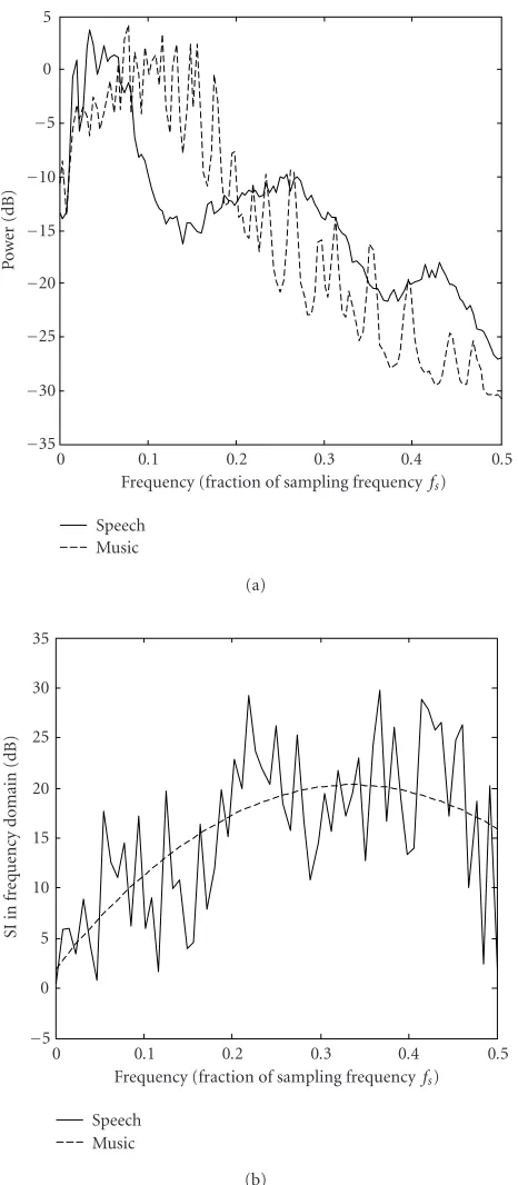
two RIRs. The difference between the spectra of the speech
and the music (shown inFigure 13a) causes different shapes
of resulting DRIRs, which ideally should be identical. Never-theless, with a single-pulse-like shape, the DRIRs still imply a strong acoustic path similarity.
Also plotted in Figure 13b is the SI values calculated
for each frequency component, where we take the resulting
DRIRs in the case ofd=10 cm andL=1024 and use white
noise as sources. The dashed line describes the average
sep-aration level for different frequencies. From there, one can
see that withd =10 cm, high frequency components of the
sources are separated better than low frequency ones. One reason is that from around 1.4 kHz down to 800 Hz, the mu-sic signal is quite dominant, and below 800 Hz the speech prevails, which is not good for separation. The other rea-son could be that the 10 cm microphone spacing provides
acoustic path differences for separation to the low frequency
components (greater than 25 cm in this particular case) not
as sufficient as to the high-frequency components. This has
been briefly discussed also at the end ofSection 4. Therefore,
depending on different acoustic environments, the
micro-phone spacing to be chosen will be always a trade-offbetween
5 0 −5 −10 −15 −20 −25 −30 −35
P
o
w
er
(dB)
0 0.1 0.2 0.3 0.4 0.5
Frequency (fraction of sampling frequencyfs)
Speech Music
(a) 35
30 25 20 15 10 5 0 −5
SI
in
fr
eq
uency
d
omain
(dB)
0 0.1 0.2 0.3 0.4 0.5
Frequency (fraction of sampling frequencyfs)
Speech Music
(b)
Figure13: (a) The spectra of the sources. (b) The frequencywise SI values.
To show the effectiveness of the BLASS algorithm for
real-world data, we design the following experiment with recorded audio signals. The signals are recorded in a room
illustrated inFigure 14with dimensions of about 3 m×4 m×
3 m (width×depth×height). The same pieces of speech and
Panel Curtain
d=20 cm
w=1 m Door
Figure14: The room for real-world audio signal recording.
music as in the synthetic data experiment are played by two loudspeakers simultaneously and recorded with two micro-phones. The microphones and loudspeakers are placed as de-picted in the figure. The panels hanging on the walls and the curtain can be flipped to choose the smooth or the coarse
side. Different combinations lead to different acoustic
envi-ronments. In this experiment, we use the coarse sides of the panels and the curtain in order to acquire a mild reverber-ation. The reverberation time, being averaged over various
positions, is T60 = 0.335 second. With different tap
num-bers Lgiven to DRIRs, the BLASS algorithm is applied to
the recorded microphone signals and the results are shown inFigure 15.
One can see that the SI curve inFigure 15areveals the
pattern similar to that inFigure 11withd=10 cm. The SI
value stays around 20 dB asLdecreases from 1024 to about
300, and the best separation appears with L ≈ 380. This
is understood when we look at the DRIRs acquired by the
BLASS in Figure 15b. They have stronger and more dense
side taps than the DRIRs obtained with synthetic data in Figure 12, but they still look quite single-pulse like, which in-dicates significant similarities existing in acoustic paths and allow the reduction of filter taps. The best SI is 5 dB lower than that with the synthetic data because of the more com-plex acoustic environment in the real world, while the corre-sponding number of taps is about 150 more since the acous-tic similarities reduce due to a larger microphone spacing
(d=20 cm).
Finally, we apply the BLASS to one of the recordings pro-vided in [31] that are normally considered as benchmarks. Two speakers have been recorded speaking simultaneously. Speaker 1 says the digits from one to ten in English and speaker 2 counts at the same time the digits in Spanish (uno,
dos, . . . ). The recording has been done in a normal office
room. The distance between the speakers and the micro-phones is about 60 cm in a square ordering. The sampling
frequency is 16 kHz. TakeL=128 andτ =τc =0 because
25
20
15
10
Separ
ation
inde
x
(dB)
0 200 400 600 800 1000
Filter taps (sample) (a)
0.4 0.2 0
−0.2
∆
h12
(
t
)
0 200 400 600 800 1000
Filter taps (sample)
0.4 0.2 0
−0.2
∆
h21
(
t
)
0 200 400 600 800 1000
Filter taps (sample) (b)
Figure15: (a) The SI versus the tap numberLgiven to DRIRs,τ= τc=0. (b) The DRIRs acquired by the BLASS.
inFigure 16. InFigure 17, we plot the two DRIRs obtained by the BLASS. Inspecting by sight or by hearing, one can hardly find any separation performance loss with the reduced filter number and shortened filter length. This confirms the
state-ment inSection 4that the proposed model is in general also
applicable to the case of large microphone spacings provided
that the filter lengthLis properly chosen.
An overview of the experiment results is given inTable 1,
whereNfilterandNcoef denote the number of filters and the
number of filter taps to be adjusted, respectively. SI loss means the separation degradation due to the use of the pro-posed model instead of a conventional model. The total
A
m
plitude
0.0 0.3 0.6 0.9 1.2 1.5 Time (s)
(a)
A
m
plitude
0.0 0.3 0.6 0.9 1.2 1.5 Time (s)
(b)
Am
p
li
tu
d
e
0.0 0.3 0.6 0.9 1.2 1.5 Time (s)
(c)
Figure16: The separation results of the real-world data. (a) Micro-phone recordings. (b) Separated signals obtained in [31]. (c) Sepa-rated signals with BLASS.
number of filter coefficients needed to achieve a
compara-ble performance is considerably reduced. In Figure 18, one
can see more generally the reduction of the needed filter taps
as the number of sources/microphonesnincreases, where
Ncoef,pro Ncoef,con =β−
β
n, (44)
Ncoef,pro and Ncoef,con represent the number of filter taps
needed for the proposed model and a conventional model,
respectively, andβis the ratio between the filter lengths used
in these two models provided that the separation perfor-mances are comparable. With a large number of sources, the
ratioNcoef,pro/Ncoef,conapproachesβ.
Table1: An overview of the experiment results regarding the reduction of the total filter taps.
Data type Mixing model Nfilter L Ncoef SL loss
Synthetic normal 4 1024 4096 negligible
proposed 2 ∼250 ∼500
Real world
Own recorded normal 4 1024 (expected) 4096 (expected) negligible
proposed 2 ∼400 ∼800
Benchmark normal 4 1024 (expected) 4096 (expected) Hardly recognized by hearing
proposed 2 128 256
0.4 0.2 0
−0.2
Am
p
li
tu
d
e
0 20 40 60 80 100 120
Filter taps (sample) (a)
0.4 0.2 0
−0.2
Am
p
li
tu
d
e
0 20 40 60 80 100 120
Filter taps (sample) (b)
Figure 17: The DRIRs acquired by the BLASS. (a) ∆h12[k].
(b)∆h21[k].
6. CONCLUSIONS
In this paper, the concept of acoustic similarities existing be-tween two propagating paths of a sound is presented. In or-der to quantitatively describe the similarity, an acoustic simi-larity index (ASI) is defined and studied. There are three ways to increase the ASI value, which are (1) reducing the micro-phone spacing, (2) making the environment less reverberant, and (3) decreasing the source-to-microphone distance. Then a new mixing model of a multispeaker-multimicrophone setup is proposed. The model is proved to be feasible in prac-tice and can be applied to simplify an audio signal separa-tion problem. With a reasonably high ASI, for example, by means of closely spacing microphones (within 5–10 cm), the model can relieve the computational load of the separation algorithm by considerably reducing the number and length of the filters to be adjusted. It is also applicable in the normal
1 0.9 0.8 0.7 0.6 0.5 0.4 0.3 0.2 0.1 0 Nco
ef
,
pr
o
/
Nco
ef
,
co
n
5 10 15 20 25
The number of sources/microphonesn β=0.75
β=0.5 β=0.25
Figure 18: Reduction of the total filter taps using the proposed model.
microphone spacings if the filters are provided with enough taps. Therefore, the implementation of a blind audio signal separation (BLASS) is used specifically for the proposed al-gorithm.
In principle, various BSS algorithms can be designed on the proposed model. As an example, in this paper, we have developed a BLASS in order to cope with real and more com-plicated situations. BLASS only uses the second-order
statis-tics and performs efficiently in frequency domain. Its eff
ec-tiveness is shown by the separation results of both synthetic and real-world signals.
REFERENCES
[1] J. Herault and C. Jutten, “Space or time adaptive signal pro-cessing by neural network models,” inNeural Networks for Computing: AIP Conference Proceedings, J. S. Denker, Ed., vol. 151, pp. 206–211, American Institute for Physics, Snowbird, Utah, USA, April 1986.
[3] K. Torkkola, “Blind separation for audio signals—are we there yet?” inProc. 1st International Workshop on Independent Com-ponent Analysis and Blind Signal Separation (ICA ’99), pp. 239–244, Aussois, France, January 1999.
[4] H.-L. N. Thi and C. Jutten, “Blind source separation for con-volutive mixtures,” Signal Processing, vol. 45, no. 2, pp. 209– 229, 1995.
[5] S. Van Gerven and D. Van Compernolle, “Signal separation by symmetric adaptive decorrelation: Stability, convergence, and uniqueness,” IEEE Trans. Signal Processing, vol. 43, no. 7, pp. 1602–1612, 1995.
[6] D. Yellin and E. Weinstein, “Multichannel signal separation: Methods and analysis,”IEEE Trans. Signal Processing, vol. 44, no. 1, pp. 106–118, 1996.
[7] J. T. Ngo and N. A. Bhadkamkar, “Adaptive blind separation of audio sources by a physically compact device using second-order statistics,” inProc. 1st International Workshop on Inde-pendent Component Analysis and Signal Separation (ICA ’99), pp. 257–260, Aussois, France, January 1999.
[8] J. Garas, Room Impulse Response, Version 2.1,http://www.
dspalgorithms.com/room/room25.html.
[9] J. B. Allen and D. A. Berkley, “Image method for efficiently simulating small-room acoustics,” Journal of the Acoustical Society of America, vol. 65, no. 4, pp. 943–950, 1979.
[10] J. Garas,Adaptive 3D sound systems, Ph.D. thesis, Eindhoven University of Technology, Eindhoven, The Netherlands, 1999. [11] V. Capdevielle, C. Serviere, and J. Lacoume, “Blind separation of wide-band sources in the frequency domain,” inProc. IEEE Int. Conf. Acoustics, Speech, Signal Processing (ICASSP ’95), pp. 2080–2083, Detroit, Mich, USA, May 1995.
[12] F. Ehlers and H. G. Schuster, “Blind separation of convolutive mixtures and an application in automatic speech recognition in noisy environment,”IEEE Trans. Signal Processing, vol. 45, no. 10, pp. 2608–2612, 1997.
[13] P. He, P. C. W. Sommen, and B. Yin, “A realtime DSP blind sig-nal separation experimental system based on a new simplified mixing model,” inProc. International Conference on Trends in Communications (EUROCON ’01), pp. 467–470, Bratislava, Slovak Republic, July 2001.
[14] P. Comon, “Independent component analysis,” inProc. Inter-national Workshop on Higher-Order Statistics (HOS ’91), pp. 111–120, Chamrousse, France, July 1991.
[15] L. Tong, R. Liu, V. Soon, and Y. Huang, “Indeterminacy and identifiability of blind identification,”IEEE Trans. Circuits and Systems, vol. 38, no. 5, pp. 499–509, 1991.
[16] J.-F. Cardoso, “Iterative techniques for blind source separa-tion using only fourth order cumulants,” inProc. 6th Euro-pean Signal Processing Conference (EUSIPCO ’92), pp. 739– 742, Brussels, Belgium, August 1992.
[17] D. Yellin and E. Weinstein, “Criteria for multichannel signal separation,” IEEE Trans. Signal Processing, vol. 42, no. 8, pp. 2158–2168, 1994.
[18] C. Jutten and J. Herault, “Blind separation of sources, part I: An adaptive algorithm based on neuromimetic architecture,”
Signal Processing, vol. 24, no. 1, pp. 1–10, 1991.
[19] J. Karhunen, L. Wang, and R. Vigario, “Nonlinear PCA type approaches for source separation and independent compo-nent analysis,” inProc. IEEE International Conference on Neu-ral Networks (ICNN ’95), pp. 995–1000, Perth, Western Aus-tralia, AusAus-tralia, November–December 1995.
[20] B. A. Pearlmutter and L. C. Parra, “Maximum likelihood blind source separation: A context-sensitive generalization of ICA,” inProc. Advances in Neural Information Processing Sys-tems (NIPS ’96), vol. 9, pp. 613–619, MIT Press, Denver, Colo, USA, December 1996.
[21] A. J. Bell and T. J. Sejnowski, “An information maximization approach to blind separation and blind deconvolution,” Neu-ral Computation, vol. 7, no. 6, pp. 1129–1159, 1995.
[22] S.-I. Amari, A. Cichocki, and H. H. Yang, “A new learning algorithm for blind signal separation,” inProc. Advances in Neural Information Processing Systems (NIPS ’96), vol. 8, pp. 757–763, MIT Press, Denver, Colo, USA, December 1996. [23] M. Girolami and C. Fyfe, “Extraction of independent signal
sources using a deflationary exploratory projection pursuit network with lateral inhibition,” IEE Proceedings on Vision, Image and Signal Processing Journal, vol. 14, no. 5, pp. 299– 306, 1997.
[24] L. Molgedey and H. Schuster, “Separation of independent sig-nals using time-delayed correlations,”Physical Review Letters, vol. 72, no. 23, pp. 3634–3637, 1994.
[25] K. Abed-Meraim, A. Belouchrani, J.-F. Cardoso, and E. Moulines, “Asymptotic performance of second order blind source separation,” inProc. IEEE Int. Conf. Acoustics, Speech, Signal Processing (ICASSP ’94), vol. 4, pp. 277–280, Adelaide, Australia, April 1994.
[26] S. Van Gerven and D. Van Compernolle, “On the use of decorrelation in scalar signal separation,” in Proc. IEEE Int. Conf. Acoustics, Speech, Signal Processing (ICASSP ’94), pp. 57–60, Adelaide, Australia, April 1994.
[27] E. Weinstein, M. Feder, and A. V. Oppenheim, “Multi-channel signal separation by decorrelation,” IEEE Trans. Speech, and Audio Processing, vol. 1, no. 4, pp. 405–413, 1993.
[28] K. Matsuoka, M. Ohya, and M. Kawamoto, “A neural net for blind separation of nonstationary signals,” Neural Networks, vol. 8, no. 3, pp. 411–419, 1995.
[29] L. Parra, C. Spence, and B. De Vries, “Convolutive blind source separation based on multiple decorrelation,” in
Proc. IEEE Workshop on Neural Networks for Signal Processing (NNSP ’98), pp. 23–32, Cambridge, UK, September 1998. [30] H. Kawahara and T. Irino, “Exploring temporal feature
repre-sentations of speech using neural networks,” Tech. Rep. SP88-31, IEICE, Tokyo, Japan, July 1988.
[31] T.-W. Lee, A. Ziehe, R. Orglmeister, and T. J. Sejnowski, “Combining time-delayed decorrelation and ICA: towards solving the cocktail party problem,” in Proc. IEEE Int. Conf. Acoustics, Speech, Signal Processing (ICASSP ’98), vol. 2, pp. 1249–1252, Seattle, Wash, USA, May 1998, Au-thors provide signals and results athttp://www.cnl.salk.edu/
∼tewon/.
[32] J. van de Laar, E. A. P. Habets, J. D. P. A. Peters, and P. A. M. Lokkart, “Adaptive blind audio signal separation on a DSP,” inProc. 12th Annual Workshop on Circuits, Systems and Sig-nal Processing (ProRISC ’01), pp. 475–479, Veldhoven, The Netherlands, November 2001.
Bin Yin received his B.S., M.S., and Ph.D. degrees in electrical engineering from Southeast University (SEU), Nanjing, China, in 1992, 1995, and 1998, respec-tively. From 1999 to 2001, as a Postdoctor, he was with the Faculty of Electrical Engineering at Eindhoven University of Technology, the Netherlands. Currently he is a Senior Scientist in Philips Research Laboratories (Nat.Lab.), Eindhoven, the
Piet C. W. Sommenreceived the Ingenieur degree in electrical engineering from Delft University of Technology in 1981 and his Ph.D. degree from Eindhoven University of Technology, the Netherlands, in 1992. From 1981 to 1989 he was with Philips Research Laboratories, Eindhoven, and since 1989, he has been with the Faculty of Electrical En-gineering at Eindhoven University of Tech-nology, where he is currently an Associate
Professor. Dr. Sommen is involved in internal and external courses, all dealing with different basic and advanced signal processing top-ics. His main field of research is in adaptive array signal processing, with applications in acoustic communication systems. Dr. Sommen is the Editor of EURASIP Newsletter.
Peiyu He received her B.S. degree from Tsinghua University, Beijing, China and her M.S. degree from Sichuan University, Chengdu, China, in 1986 and 1989, re-spectively. From 2000 to 2001, she was with the Faculty of Electrical Engineering at Eindhoven University of Technology, the Netherlands, as a visiting Researcher. Cur-rently she is Professor in Sichuan University, Chengdu, China. Her main field of research