Physically Informed Signal Processing Methods
for Piano Sound Synthesis: A Research Overview
Bal ´azs Bank
Department of Measurement and Information Systems, Faculty of Electronical Engineering and Informatics, Budapest University of Technology and Economics, H-111 Budapest, Hungary
Email:[email protected]
Federico Avanzini
Department of Information Engineering, University of Padova, 35131 Padua, Italy Email:[email protected]
Gianpaolo Borin
Dipartimento di Informatica, University of Verona, 37134 Verona, Italy Email:[email protected]
Giovanni De Poli
Department of Information Engineering, University of Padova, 35131 Padua, Italy Email:[email protected]
Federico Fontana
Department of Information Engineering, University of Padova, 35131 Padua, Italy Email:[email protected]
Davide Rocchesso
Dipartimento di Informatica, University of Verona, 37134 Verona, Italy Email:[email protected]
Received 31 May 2002 and in revised form 6 March 2003
This paper reviews recent developments in physics-based synthesis of piano. The paper considers the main components of the instrument, that is, the hammer, the string, and the soundboard. Modeling techniques are discussed for each of these elements, to-gether with implementation strategies. Attention is focused on numerical issues, and each implementation technique is described in light of its efficiency and accuracy properties. As the structured audio coding approach is gaining popularity, the authors argue that the physical modeling approach will have relevant applications in the field of multimedia communication.
Keywords and phrases:sound synthesis, audio signal processing, structured audio, physical modeling, digital waveguide, piano.
1. INTRODUCTION
Sounds produced by acoustic musical instruments can be described at thesignallevel, where only the time evolution of the acoustic pressure is considered and no assumptions on the generation mechanism are made. Alternatively,source models, which are based on a physical description of the sound production processes [1,2], can be developed.
Physics-based synthesis algorithms provide semantic sound representations since the control parameters have a straightforward physical interpretation in terms of masses,
springs, dimensions, and so on. Consequently, modification of the parameters leads in general to meaningful results and allows more intuitive interaction between the user and the virtual instrument. The importance of sound as a primary vehicle of information is being more and more recognized in the multimedia community. Particularly, source models of sounding objects (not necessarily musical instruments) are being explored due to their high degree of interactivity and the ease in synchronizing audio and visual synthesis [3].
where, in addition to the parameters, the decoding algo-rithm is transmitted to the user as well. The structured audio orchestral language (SAOL) became a part of the MPEG-4 standard, thus it is widely available for multimedia applica-tions. Known problems in using physical models for coding purposes are primarily concerned with parameter estima-tion. Since physical models describe specific classes of instru-ments, automatic estimation of the model parameters from an audio signal is not a straightforward task: the model struc-ture which is best suited for the audio signal has to be chosen before actual parameter estimation. On the other hand, once the model structure is determined, a small set of parameters can describe a specific sound. Casey [6] and Serafin et al. [7] address these issues.
In this paper, we review some of the strategies and al-gorithms of physical modeling, and their applications to pi-ano simulation. The pipi-ano is a particularly interesting instru-ment, both for its prominence in western music and for its complex structure [8]. Also, its control mechanism is simple (it basically reduces to key velocity), and physical control de-vices (MIDI keyboards) are widely available, which is not the case for other instruments. The source-based approach can be useful not only for synthesis purposes but also for gaining a better insight into the behavior of the instruments. How-ever, as we are interested in efficient algorithms, the features modeled are only those considered to have audible effects. In general, there is a trade-offbetween the accuracy and the simplicity of the description. The optimal solution may vary depending on the needs of the user.
The models described here are all based ondigital waveg-uides. The waveguide paradigm has been found to be the most appropriate for real-time synthesis of a wide range of musical instruments [9,10,11]. As early as in 1987, Gar-nett [12] presented a physical waveguide piano model. In his model, a semiphysical lumped hammer is connected to a dig-ital waveguide string and the soundboard is modeled by a set of waveguides, all connected to the same termination.
In 1995, Smith and Van Duyne [13, 14] presented a model based on commuted synthesis. In their approach, the soundboard response is stored in an excitation table and fed into a digital waveguide string model. The hammer is modeled as a linear filter whose parameters depend on the hammer-string collision velocity. The hammer filter param-eters have to be precalculated and stored for all notes and hammer velocities. This precalculation can be avoided by running an auxiliary string model connected to a nonlinear hammer model in parallel, and, based on the force response of the auxiliary model, designing the hammer filters in real time [15].
The original motivation for commuted synthesis was to avoid the high-order filter which is needed for high qual-ity soundboard modeling. As low-complexqual-ity methods have been developed for soundboard modeling (see Section 5), the advantages of the commuted piano with respect to the direct modeling approach described here are reduced. Also, due to the lack in physical description, some effects, such as the restrike (ribattuto) of the same string, cannot be precisely modeled with the commuted approach. Describing the
com-muted synthesis in detail is beyond the scope of this paper, although we would like to mention that it is a comparable alternative to the techniques described here.
As part of a collaboration between the University of Padova and Generalmusic, Borin et al. [16] presented a complete real-time piano model in 1997. The hammer was treated as a lumped model, with a mass connected in paral-lel to a nonlinear spring, and the strings were simulated us-ing digital waveguides, all connected to a sus-ingle-lumped load. Bank [17] introduced in 2000 a similar physical model, based on the same functional blocks, but with slightly different im-plementation. An alternative approach was used for the solu-tion of the hammer differential equation. Independent string models were used without any coupling, and the influence of the soundboard on decay times was taken into account by using high-order loss filters. The use of feedback delay networks was suggested for modeling the radiation of the soundboard.
This paper addresses the design of each component of a piano model (i.e., hammer, string, and soundboard). Dis-cussion is carried on with particular emphasis on real-time applications, where the time complexity of algorithms plays a key role. Perceptual issues are also addressed since a precise knowledge of what is relevant to the human ear can drive the accuracy level of the design.Section 2deals with general aspects of piano acoustics. InSection 3, the hammer is dis-cussed and numerical techniques are presented to overcome the computability problems in the nonlinear discretized sys-tem.Section 4is devoted to string modeling, where the prob-lems of parameter estimation are also addressed. Finally, Section 5deals with the soundboard, where various alterna-tive techniques are described and the use of the multirate ap-proach is proposed.
2. ACOUSTICS AND MODEL STRUCTURE
Piano sounds are the final product of a complex synthesis process which involves the entire instrument body. As a result of this complexity, each piano note exhibits its unique sound features and nuances, especially in high quality instruments. Moreover, just varying the impact force on a single key al-lows the player to explore a rich dynamic space. Accounting for such dynamic variations in a wavetable-based synthesizer is not trivial: dynamic postprocessing filters which shape the spectrum according to key velocity can be designed, but find-ing a satisfactory mappfind-ing from velocity to filter response is far from being an easy task. Alternatively, a physical model, which mimics as closely as possible the acoustics of the in-strument, can be developed.
String Bridge
Hammer Soundboard
(a)
Excitation
Control
String Radiator Sound
(b)
Figure1: General structures: (a) schematic representation of the instrument and (b) model structure.
Since the physical modeling approach tries to simulate the structure of the instrument rather than the sound itself, the blocks in the piano model resemble the parts of a real pi-ano. The structure is displayed inFigure 1b. The first model block is the excitation, the hammer strike. Its output prop-agates to the string, which determines the fundamental fre-quency of the tone. The quasiperiodic output signal is fil-tered through a postprocessing block, covering the radiation effects of the soundboard.Figure 1bshows that the hammer-string interaction is bidirectional since the hammer force de-pends on the string displacement [8]. On the other hand, there is no feedback from the radiator to the string. Feed-back and coupling effects on the bridge and the soundboard are taken into account in the string block. The model differs from a real piano in the fact that the two functions of the soundboard, namely, to provide a terminating impedance to the strings and to radiate sound, are located in separate parts of the model. As a result, it is possible to treat radiation as a linear filtering operation.
3. THE HAMMER
We will first discuss the physical aspects of the hammer-string interaction, then concentrate on various modeling ap-proaches and implementation issues.
3.1. Hammer-string interaction
As a first approximation, the piano hammer can be consid-ered a lumped mass connected to a nonlinear spring, which is described by the equation
F(t)= −mh d2yh(t)
dt2 , (1)
whereF(t) is the interaction force and yh(t) is the hammer displacement. The hammer mass is represented by mh. Ex-periments on real instruments have shown (see, e.g., [18,19, 20]) that the hammer-string contact can be described by the following formula:
Table1: Sample values for hammer parameters for three different notes, taken from [19,20]. The hammer massmhis given in kg.
C2 C4 C6
p 2.3 2.5 3
k 4.0×10⁸ 4.5×10⁹ 1.0×10¹²
mh 4.9×10⁻³ 2.97×10⁻³ 2.2×10⁻³
F(t)= f∆y(t)=
k∆y(t)p, ∆y(t)>0,
0, ∆y(t)≤0, (2)
where∆y(t)=yh(t)−ys(t) is the compression of the ham-mer felt, ys(t) is the string position,k is the hammer stiff -ness coefficient, and pis the stiffness exponent. The condi-tion ∆y(t) > 0 corresponds to the hammer-string contact, while the condition ∆y(t) ≤ 0 indicates that the hammer is not touching the string. Equations (1) and (2) result in a nonlinear differential system of equations foryh(t). Due to the nonlinearity, the tone spectrum varies dynamically with hammer velocity. Typical values of hammer parameters can be found in [19,20]. Example values are listed inTable 1.
However, (2) is not fully satisfactory in that real piano hammers exhibit hysteretic behavior. That is, contact forces during compression and during decompression are different, and a one-to-one law between compression and force does not correspond to reality. A general description of the hys-teresis effect of piano felts was provided by Stulov [21]. The idea, coming from the general theory of mechanics of solids, is that the stiffnesskof the spring in (2) has to be replaced by a time-dependent operator which introduces memory in the nonlinear interaction. Thus, the first part of (2) (when ∆y(t)>0) is replaced by
F(t)=f∆y(t)=k1−hr(t)∗∆y(t)p, (3)
wherehr(t)=(/τ)e−t/τis arelaxation functionthat accounts for the “memory” of the material and the∗operator repre-sents convolution.
Previous studies [22] have shown that a good fit to real data can be obtained by implementinghras a first-order low-pass filter. It has to be noted that informal listening tests in-dicate that taking into account the hysteresis in the hammer model does not improve the sound quality significantly.
3.2. Implementation approaches
The theory of wave digital filters addresses the problem of noncomputable loops in terms of wave variables. Every com-ponent of a circuit is described as a scattering element with a reference impedance, and delay-free loops between com-ponents are treated by “adapting” reference impedances. Van Duyne et al. [23] presented a “wave digital hammer” model, where wave variables are used. More severe computability problems can arise when simulating nonlinear dynamic ex-citers since the linear equations used to describe the system dynamics are tightly coupled with a nonlinear map. Borin et al. [24] have recently proposed a general strategy named “Kmethod” for solving noncomputable loops in a wide class of nonlinear systems. The method is fully described in [24] along with some application examples. Here, only the basic principles are outlined.
Whichever the discretization method is, the hammer compression∆y(n) at timencan be written as
∆y(n)=p(n) +KF(n), (4)
where p(n) is the linear combination of past values of the variables (namely,yh,ys, andF) andKis a coefficient whose value depends on the numerical method in use. The inter-action forceF(n) at discrete time instantn, computed either by (2) or (3), is therefore described by the implicit relation F(n) = f(p(n) +KF(n)). TheK method uses the implicit function theorem to solve the following implicit relation:
F=f(p+KF)K−→meth.F=h(p). (5)
The new nonlinear map h defines F as a function of p, hence instantaneous dependencies across the nonlinearity are dropped. The functionhcan be precomputed and stored in a lookup table for efficient implementation.
Bank [25] presented a simpler but less general method for avoiding artifacts caused by fictitious delay insertion. The idea is that the stability of the discretized hammer model with a fictitious delay can always be maintained by choos-ing a sufficiently large sampling rate fsif the corresponding continuous-time system is stable. As fs → ∞, the discrete-time system will behave as the original differential equation. Doubling the sampling rate of the whole string model would double the computation time as well. However, if only the hammer model operates at double rate, the computational complexity is raised only by a negligible amount. Therefore, in the proposed solution, the hammer operates at twice sam-pling rate of the string. Data is downsampled using sim-ple averaging and upsamsim-pled using linear interpolation. The multirate hammer has been found to result in well-behaving force signals at a low-computational cost. As the hammer model is a nonlinear dynamic system, the stability bounds are not trivial to derive in a closed form. In practice, stability is maintained up to an impact velocity ten times higher than the point where the straightforward approach (e.g., used in [19,20]) turns unstable.
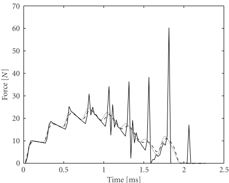
Figure 2shows a typical force signal in a hammer-string contact. The overall contact duration is around 2 ms and the pulses in the signal are produced by reflections of force
70 60 50 40 30 20 10 0
Fo
rc
e
[
N
]
0 0.5 1 1.5 2 2.5
Time [ms]
Figure 2: Time evolution of the interaction force for note C5
(522 Hz) withfs=44.1 kHz, and hammer velocityv=5 m/s, com-puted by inserting a fictitious delay element (solid line), with the
K method (dashed line), and with the multirate hammer (dotted line).
waves at string terminations. TheKmethod and the multi-rate hammer produce very similar force signals. On the other hand, inserting a fictitious delay element drives the system towards instability (the spikes are progressively amplified). In general, the multirate method provide results comparable to theKmethod for hammer parameters realistic for pianos, while it does not require that precomputed lookup tables be stored. On the other hand, when low-sampling rates (e.g., fs = 11.025 kHz) or extreme hammer parameters are used (i.e.,kis ten times the value listed inTable 1), the system sta-bility cannot be maintained by upsampling by a factor of 2. In such cases, theKmethod is the appropriate solution.
The computational approaches presented in this section are applicable to a wide class of mechanical interactions be-tween physical objects [26].
4. THE STRING
Many different approaches have been presented in the litera-ture for string modeling. Since we are considering techniques suitable for real-time applications, only the digital waveguide [9,10,11] is described here in detail. This method is based on the time-domain solution of the one-dimensional wave equation. The velocity distribution of the stringv(x, t) can be seen as the sum of two traveling waves:
v(x, t)=v+(x−ct) +v−(x+ct), (6)
wherexdenotes the spatial coordinate,tis time,cis the prop-agation speed, andv+andv−are the traveling wave compo-nents.
−1
z−Min + Min
z−(M−Min) M
Fout
Fin Hr(z)
z−Min + z−(M−Min)
Figure3: Digital waveguide model of a string with one polariza-tion.
and dispersion can be consolidated to one end of the digi-tal waveguide [9,10,11]. In the case of one polarization of a piano string, the system takes the form shown inFigure 3, whereM represents the length of the string in spatial sam-pling intervals,Min denotes the position of the force input,
andHr(z) refers to the reflection filter. This structure is ca-pable of generating a set of quasiharmonic, exponentially de-caying sinusoids. Note that the four delay lines of Figure 3 can be simplified to a two-delay line structure for more effi -cient implementation [13].
Accurate design of the reflection filter plays a key role for creating realistic sounds. To simplify the design, Hr(z) is usually split into three separate parts: Hr(z) = −Hl(z)Hd(z)Hf d(z), where Hl(z) accounts for the losses, Hd(z) for the dispersion due to stiffness, andHf d(z) for fine-tuning the fundamental frequency. Using allpass filtersHd(z) for simulating dispersion ensures that the decay times of the partials are controlled by the loss filterHl(z) only. The slight phase difference caused by the loss filter is negligible com-pared to the phase response of the dispersion filter. In this way, the loss filter and the dispersion filter can be treated as orthogonal with respect to design.
The string needs to be fine tuned because delay lines can implement only an integer phase delay and this provides too low resolution for the fundamental frequencies. Fine tuning can be incorporated in the dispersion filter design or, alter-natively, a separate fractional delay filterHf d(z) can be used in series with the delay line. Smith and Jaffe [9,27] suggested to use a first-order allpass filter for this purpose. V¨alim¨aki et al. [28] proposed an implementation based on low-order Lagrange interpolation filters. Laakso et al. [29] provided an exhaustive overview on this topic.
4.1. Loss filter design
First, the partial envelopes of the recorded note have to be calculated. This can be done by sinusoidal peak tracking with short time Fourier transform implementation [28] or by heterodyne filtering [30]. A robust way of calculating de-cay times is fitting a line by linear regression on the logarithm of the amplitude envelopes [28]. The magnitude specifica-tiongkfor the loss filter can be computed as follows:
gk=Hl
ej(2π fk/ fs)=e−k/ fkτk, (7)
where fkandτkare the frequency and the decay time of the kth partial, and fsis the sampling rate. Fitting a filter to thegk
coefficients is not trivial since the error in the decay times is a nonlinear function of the filter magnitude error. If the mag-nitude response exceeds unity, the digital waveguide loop be-comes unstable. To overcome this problem, V¨alim¨aki et al. [28, 30] suggested the use of a one-pole loop filter whose transfer function is
H1p(z)=g 1 +a1
1 +a1z−1.
(8)
The advantage of this filter is that stability constraints for the waveguide loop, namely, a1 < 0 and 0 < g < 1, are
rela-tively simple. As for the design, V¨alim¨aki et al. [28,30] used a simple algorithm for minimizing the magnitude error in the mean squares sense. However, the overall decay time of the synthesized tone did not always coincide with the origi-nal one.
As a general solution for loss filter design, Smith [9] sug-gested to minimize the error of decay times of the partials rather than the error of the filter magnitude response. This assures that the overall decay time of the note is preserved and the stability of the feedback loop is maintained. More-over, optimization with respect to decay times is perceptu-ally more meaningful. The methods described hereafter are all based on this idea.
Bank [17] developed a simple and robust method for one-pole loop filter design. The approximate analytical for-mulas for decay timesτkof a digital waveguide with a one-pole filter are as follows:
τk≈ 1 c1+c3ϑ2k
, (9)
where c1 andc3 are computed from the parameters of the
one-pole filter of (8):
c1= f0(1−g), c3= −f0 a1
2a1+ 1
2, (10)
where f0is the fundamental frequency andϑk =2π fk/ fsis the digital frequency of thekth partial in radians. Equation (9) shows that the decay rate σk = 1/τk is a second-order polynomial of frequencyϑkwith even order terms. This sim-plifies the filter design sincec1andc3are easily determined
by polynomial regression from the prescribed decay times. A weighting function ofwk=τk4has to be used to minimize the error with respect toτk. Parametersganda1of the one-pole
loop filter are easily computed via the inverse of (10) from coefficientsc1andc3.
Another approach was proposed by Bank [17] who sug-gested the transformation of the specification. As the goal is to match decay times, the magnitude specificationgkis trans-formed into a formgk,tr=1/(1−gk) which approximatesτk,
and a transformed filterHtr(z) is designed for the new
spec-ification by least squares filter design. The loss filterHl(z) is then computed by the inverse transformHl(z)=1−1/Htr(z).
Bank and V¨alim¨aki [32] presented a simpler method for high-order filter design based on a special weighting func-tion. The resulting decay times of the digital waveguide are computed from the magnitude response ˆgk = |H(ejϑk)|of the loss filter by ˆτk = d( ˆgk) = −1/(f0ln ˆgk). This function
is approximated by its first-order Taylor series around the specification d( ˆgk) ≈ d(gk) +d( ˆgk −gk). Accordingly, the error with respect to decay times can be approximated by the weighted mean square error
The weighted erroreWLScan be easily minimized by standard
filter design algorithms, and leads to a good match with re-spect to decay times.
All of these techniques for high-order loss filter design have been found to be robust in practice. Comparing them is left for future work.
Borin et al. [16] have used a different approach for mod-eling the decay time variations of the partials. In their im-plementation, second-order FIR filters are used as loss filters that are responsible for the general decay of the note. Small variations of the decay times are modeled by connecting all the string models to a common termination which is imple-mented as a filter with a high number of resonances. This also enables the simulation of the pedal effect since now all the strings are coupled to each other (see Section 4.3). An advantage of this method compared to high-order loop fil-ters is the smaller computational complexity. On the other hand, the partial envelopes of the different notes cannot be controlled independently.
Although optimizing the loss filter with respect to de-cay times has been found to give perceptually adequate re-sults, we remark that the loss filter design can be helped via perceptual studies. The audibility of the decay-time varia-tions for the one-pole loss filter was studied by Tolonen and J¨arvel¨ainen [33]. The study states that relatively large devia-tions (between−25% and +40%) in the overall decay time of the note are not perceived by listeners. Unfortunately, the-oretical results are not directly applicable for the design of high-order loss filters as the tolerance for the decay time vari-ations of single partials is not known.
4.2. Dispersion simulation
Dispersion is due to stiffness which causes piano strings to deviate from ideal behavior. If the dispersive correction term in the wave equation is small, its first-order effect is
to increase the wave propagation speedc(f) with frequency. This phenomenon causes string partials to become inhar-monic. If the string parameters are known, then the fre-quency of thekth stretched partial can be computed as
fk=k f0
1 +Bk2, (12)
where the value of the inharmonicity coefficientBdepends on the parameters of the string (see, e.g., [34]).
Phase delay specificationDd(fk) for the dispersion filter Hd(z) can be computed from the partial frequencies:
Dd
whereN is the total length of the waveguide delay line and Dl(fk) is the phase delay of the loss filterHl(z). The phase specification of the dispersion filter becomes φpre(fk) =
2π fkDd(fk)/ fs.
Van Duyne and Smith [35] proposed an efficient method for simulating dispersion by cascading equal first-order all-pass filters in the waveguide loop; however, the constraint of using equal first-order sections is too severe and does not al-low accurate tuning of inharmonicity.
Rocchesso and Scalcon [36] proposed a design method based on [37]. Starting from a target phase response,lpoints {fk}k=1,...,lare chosen on the frequency axis corresponding to the points where string partials should be located. The filter order is chosen to ben < l. For each partialk, the method
whereφpre(f) is the prescribed allpass response. Filter coeffi
-cientsajare computed by solving the system
n
A least-squared equation error (LSEE) is used to solve the overdetermined system (15). It was shown in [36] that sev-eral tens of partials can be correctly positioned for any piano key, with the allpass filter order not exceeding 20. Moreover, the fine tuning of the string is automatically taken into ac-count in the design. Figure 4plots results obtained using a filter order of 18. Note that the pure tone frequency JND (just noticeable difference) has been used inFigure 4bas a refer-ence as no accurate studies of partial JNDs for piano tones are available to our knowledge.
35 30 25 20 15 10 5 0
P
er
centage
dispersion
(%)
0 10 20 30 40 50 60 70 80 90 100
Order of partial numbers (a)
40 30 20 10 0
−10
−20
−30
−40
De
vi
ation
o
f
p
ar
tials
(c
ent)
0 1000 2000 3000 4000 5000 6000
Frequency (Hz) (b)
Figure4: Dispersion filter (18th order) for theC2string: (a)
com-puted (solid line) and theoretical (dashed line) percentage disper-sion versus partial numbers and (b) deviation of partials (solid line). Dash-dotted vertical lines show the end of the LSEE approximation; dash-dotted bounds in (b) indicate the pure tone frequency JND as a reference; and the dashed line in (b) is the partial deviation from the theoretical inharmonic series in a nondispersive string model.
logarithmic pitch scale. Partials above this frequency band only contribute some brightness to the sound, and can be made harmonic without relevant perceptual consequences.
J¨arvel¨ainen et al. [39] also found that inharmonicity is more easily perceived at low frequencies even when coeffi -cientBfor bass tones is lower than for treble tones. This is probably due to the fact that beats are used by listeners as cues for inharmonicity, and even low B’s produce enough mistuning in higher partials of low tones. These findings can help in the allpass filter design procedure, although a number of issues still need further investigation.
Fin
Sv(z) + Fout
↓2 R1(z) + ↑2
↓2 R2(z) + ↑2
. . .
. .
. ...
↓2 Rk(z) ↑2
Figure5: The multirate resonator bank.
As high-order dispersion filters are needed for modeling low notes, the computational complexity is increased signifi-cantly. Bank [17] proposed a multirate approach to overcome this problem. Since the lowest tones do not contain signifi-cant energy in the high-frequency region anyway, it is worth-while to run the lowest two or three octaves of the piano at half-sampling rate of the model. The outputs of the low notes are summed before upsampling, therefore only one interpo-lation filter is required.
4.3. Coupled piano strings
String coupling occurs at two different levels. First of all, two or three slightly mistuned strings are sounded together when a single piano key is pressed (except for the lowest octave) and complicated modulation of the amplitudes is brought about. This results in beating and two-stage decay, the first refers to an amplitude modulation overlaid on the exponen-tial decay, and the latter means that tone decays are faster in the early part than in the latter. These phenomena were stud-ied by Weinreich as early as in 1977 [40]. At the second level, the presence of the bridge and the action of the soundboard is known to originate important coupling effects even between different tones. In fact, the bridge-soundboard system con-nects strings together and acts as a distributed driving-point impedance for string terminations.
The simplest way for modeling beating and two-stage de-cay is to use two digital waveguides in parallel for a single note. Varying by the used type of coupling, many different solutions have been presented in the literature, see, for ex-ample, [14,41].
Bank [17] presented a different approach for modeling beating and two-stage decay, based on a parallel resonator bank. In a subsequent study, the computational complexity of the method was decreased by an order of ten by applying multirate techniques, making the approach suitable for real-time implementations [42]. In this approach, second-order resonatorsR1(z)· · ·Rk(z) are connected to the basic string
one by one of the resonatorsRk(z). The transfer functions of the resonators are as follows:
Rk(z)= Re tial phase, frequency, and decay-time parameters of thekth resonator, respectively. The overline stands for complex con-jugation, Re indicates the real part of a complex variable, and
fsis the sampling frequency.
An advantage of the structure is that the resonatorsRk(z) are implemented only for those partials whose beating and two-stage decay are prominent. The others will have sim-ple exponential decay, determined by the digital waveguide model Sv(z). Five to ten resonators have been found to be enough for high-quality sound synthesis. The resonator bank is implemented by the multirate approach, running the res-onators at a much lower-sampling rate, for example, the 1/8 or 1/16 part of the original sampling frequency.
It is shown in [42] that when only half of the downsam-pled frequency band is used for resonators, no lowpass filter-ing is needed before downsamplfilter-ing. This is due to the fact that the excitation signal is of lowpass character leading to aliasing less than−20 dB. As the role of the excitation signal is to set the initial amplitudes and phases of the resonators, the result of this aliasing is a less than 1 dB change in the res-onator amplitudes, which has been found to be inaudible. On the other hand, the interpolation filters after upsampling cannot be neglected. However, they are not implemented for all notes separately; the lower-sampling rate signals of the dif-ferent strings are summed before interpolation filtering (this is not depicted in Figure 5). Their specification is relatively simple (e.g., 5 dB passband ripple) since their passband er-rors can be easily corrected by changing the initial ampli-tudes and phases of the resonators. This results in signifi-cantly lower-computational cost, compared to the methods which use coupled waveguides.
Generally, the average computational cost of the method for one note is less than five multiplications per sample. Moreover, the parameter estimation gets simpler since only the parameters of the mode pairs have to be found by, for example, the methods presented in [17,41], and there is no need for coupling filter design. Stability problems of a cou-pled system are also avoided. The method presented here shows that combining physical and signal-based approaches can be useful in reducing computational complexity.
Modeling the coupling between strings of different tones is essential when the sustain pedal effect has to be simu-lated. Garnett [12] and Borin et al. [16] suggested connect-ing the strconnect-ings to the same lumped terminatconnect-ing impedance. The impedance is modeled by a filter with a high number of peaks. For that, the use of feedback delay networks [43,44] is a good alternative. Although in real pianos the bridge con-nects to the string as a distributed termination, thus coupling different strings in different ways, the simple model of Borin et al. was able to produce a realistic sustain pedal effect [45].
5. RADIATION MODELING
The soundboard radiates and filters the string waves that reach the bridge, and radiation patterns are essential for describing the “presence” of a piano in a musical context. However, now we are concentrating on describing the sound pressure generated by the piano at a certain locus in the listening space, that is, the directional properties of radia-tion are not taken into account. Modeling the soundboard as a linear postprocessing stage is an intrinsically weak ap-proach since on a real piano it also accounts for coupling between strings and affects the decay times of the partials. However, as already stated inSection 2, our modeling strat-egy keeps theradiationproperties of the soundboard sepa-rated from itsimpedanceproperties. The latter are incorpo-rated in the string model, and have already been addressed in Sections4.1and4.3; here we will concentrate on radia-tion.
A simple and efficient radiation model was presented by Garnett [12]. The waveguide strings were connected to the same termination and the soundboard was simulated by con-necting six additional waveguides to the common termina-tion. This can be seen as a predecessor of using feedback de-lay networks for soundboard simulation. Feedback dede-lay net-works have been proven to be efficient in simulating room reverberation since they are able to produce high-modal density at a low-computational cost [43]. For an overview, see the work of Rocchesso and Smith [44]. Bank [17] ap-plied feedback delay networks with shaping filters for the simulation of piano soundboards. The shaping filters were parametrized in such a way that the system matched the over-all magnitude response of a real piano soundboard. A draw-back of the method is that the modal density and the quality factors of the modes are not fully controllable. The method has proven to yield good results for high piano notes, where simulating the attack noise (the knock) of the tone is the most important issue.
The problem of soundboard radiation can also be ad-dressed from the point of view of filter design. However, as the soundboard exhibits high-modal density, a high-order filter has to be used. For fs = 44.1 kHz, a 2000 tap FIR fil-ter was necessary to achieve good results. The filfil-ter order did not decrease significantly when IIR filters were used.
To resolve the high-computational complexity, a multi-rate soundboard model was proposed by Bank et al. [46]. The structure of the model is depicted inFigure 6. The string signal is split into two parts. The part below 2.2 kHz is down-sampled by a factor of 8 and filtered by a high-order fil-ter Hlow(z) precisely synthesizing the amplitude and phase
response of the soundboard for the low frequencies. The part above 2.2 kHz is filtered by a low-order filter, model-ing the overall magnitude response of the soundboard at high frequencies. The signal of the high-frequency chain is delayed by N samples to compensate for the latency of decimation and interpolation filters of the low-frequency chain.
The filters Hlow(z) and Hhigh(z) are computed as
measuring the force-pressure transfer function of a real piano soundboard. Then, this is lowpass-filtered and downsampled by a factor of 8 to produce an FIR filterHlow(z). The impulse
response of the low-frequency chain is now subtracted from the target responseHt(z) providing a residual response con-taining energy above 2.2 kHz. This residual response is made minimum phase and windowed to a short length (50 tap). The multirate soundboard model outlined here consumes 100 operations per cycle and produces a spectral character similar to that of a 2000-tap FIR filter. The only difference is that the attack of high notes sounds sharper since the en-ergy of the soundboard response is concentrated to a short time period above 2.2 kHz. This could be overcome by using feedback delay networks forHhigh(z), which is left for future
research.
The parameters of the multirate soundboard model can-not be interpreted physically. However, this does can-not lead to any drawbacks since the parameters of the soundboard can-not be changed by the player in real pianos either. Having a purely physical model, for example, based on finite diff er-ences [47], would lead to unacceptable high-computational costs. Therefore, implementing a black box model block as a part of a physical instrument model seems to be a good com-promise.
6. CONCLUSIONS
This paper has reviewed the main stages of the development of a physical model for the piano, addressing computational aspects and discussing problems that not only are related to piano synthesis but arise in a broad class of physical models of sounding objects.
Various approaches have been discussed for dealing with nonlinear equations in the excitation block. We have pointed out that inaccuracies at this stage can lead to severe instabil-ity problems. Analogous problems arise in other mechanical and acoustical models, such as impact and friction between two sounding objects, or reed-bore interaction. The two al-ternative solutions presented for the piano hammer can be used in a wide range of applications.
Several filter design techniques have been reviewed for the accurate tuning of the resonating waveguide block. It has been shown that high-order dispersion filters are needed for accurate simulation of inharmonicity. Therefore, perceptual issues have been addressed since they are helpful in optimiz-ing the design and reducoptimiz-ing computational loads. The re-quirement of physicality can always be weakened when the effect caused by a specific feature is considered to be inaudi-ble.
A filter-based approach was presented for the sound-board model. As such, it cannot be interpreted as physical, but this does not influence the functionality of the model. In general, only those parameters which are involved in block interaction or are influenced by control messages need to have a clear physical interpretation. Therefore, we recom-mend synthesis structures that are based on building blocks with physical input and output parameters, but whose inner
Fstring ↓8 Hlow(z) ↑8 + P
Hhigh(z) z−N
Figure6: The multirate soundboard model.
structure does not necessarily follow physical model. In other words, the basic building blocks are black box models with the most efficient implementations available, and they form the physical structure of the instrument model at a higher level.
The use of multirate techniques was suggested for mod-eling beating and two-stage decay as well as the soundboard. The model can run at different sampling rates (e.g., 44.1, 22.05, and 11.025 kHz) or/and with different filter orders im-plemented in the digital waveguide model. Since the stabil-ity of the numerical structures is maintained in all cases, the user has the option of choosing between quality and effi -ciency. This remark is also relevant for potential applications in structured audio coding. In cases when instrument mod-els are to be encoded and transmitted without the precise knowledge of the computational power of the decoder, it is essential that the stability is guaranteed even at low-sampling rates in order to allow graceful degradation.
ACKNOWLEDGMENTS
Work at CSC-DEI, University of Padova, was developed un-der a Research Contract with Generalmusic. Partial fund-ing was provided by the EU Project “MOSART,” Improvfund-ing Human Potential, and the Hungarian National Scientific Re-search Fund OTKA F035060. The authors are thankful to P. Hussami and to the anonymous reviewers for their helpful comments, which have contributed to the improvement of the paper.
REFERENCES
[1] G. De Poli, “A tutorial on digital sound synthesis techniques,” inThe Music Machine, C. Roads, Ed., pp. 429–447, MIT Press, Cambridge, Mass, USA, 1991.
[2] J. O. Smith III, “Viewpoints on the history of digital synthe-sis,” inProc. International Computer Music Conference (ICMC ’91), pp. 1–10, Montreal, Quebec, Canada, October 1991. [3] K. Tadamura and E. Nakamae, “Synchronizing computer
graphics animation and audio,” IEEE Multimedia, vol. 5, no. 4, pp. 63–73, 1998.
[4] E. D. Scheirer, “Structured audio and effects processing in the MPEG-4 multimedia standard,” Multimedia Systems, vol. 7, no. 1, pp. 11–22, 1999.
[5] B. L. Vercoe, W. G. Gardner, and E. D. Scheirer, “Structured audio: creation, transmission, and rendering of parametric sound representations,” Proceedings of the IEEE, vol. 86, no. 5, pp. 922–940, 1998.
[7] S. Serafin, J. O. Smith III, and H. Thornburg, “A pattern recognition approach to invert a bowed string physical model,” inProc. International Symposium on Musical Acoustics (ISMA ’01), pp. 241–244, Perugia, Italy, September 2001. [8] N. H. Fletcher and T. D. Rossing, The Physics of Musical
In-struments, Springer-Verlag, New York, NY, USA, 1991. [9] J. O. Smith III, Techniques for digital filter design and system
identification with application to the violin, Ph.D. thesis, De-partment of Music, Stanford University, Stanford, Calif, USA, June 1983.
[10] J. O. Smith III, “Principles of digital waveguide models of mu-sical instruments,” inApplications of Digital Signal Processing to Audio and Acoustics, M. Kahrs and K. Brandenburg, Eds., pp. 417–466, Kluwer Academic, Boston, Mass, USA, 1998. [11] J. O. Smith III,Digital Waveguide Modeling of Musical
Instru-ments, August 2002, http://www-ccrma.stanford.edu/∼jos/ waveguide/.
[12] G. E. Garnett, “Modeling piano sound using waveguide digi-tal filtering techniques,” inProc. International Computer Music Conference (ICMC ’87), pp. 89–95, Urbana, Ill, USA, Septem-ber 1987.
[13] J. O. Smith III and S. A. Van Duyne, “Commuted piano synthesis,” inProc. International Computer Music Conference (ICMC ’95), pp. 335–342, Banff, Canada, September 1995. [14] S. A. Van Duyne and J. O. Smith III, “Developments for
the commuted piano,” inProc. International Computer Music Conference (ICMC ’95), pp. 319–326, Banff, Canada, Septem-ber 1995.
[15] B. Bank and L. Sujbert, “On the nonlinear commuted syn-thesis of the piano,” inProc. 5th International Conference on Digital Audio Effects (DAFx ’02), pp. 175–180, Hamburg, Ger-many, September 2002.
[16] G. Borin, D. Rocchesso, and F. Scalcon, “A physical piano model for music performance,” inProc. International Com-puter Music Conference (ICMC ’97), pp. 350–353, Thessa-loniki, Greece, September 1997.
[17] B. Bank, “Physics-based sound synthesis of the piano,” M.S. thesis, Department of Measurement and Information Sys-tems, Budapest University of Technology and Economics, Bu-dapest, Hungary, May 2000, published as Tech. Rep. 54, Lab-oratory of Acoustics and Audio Signal Processing, Helsinki University of Technology, Helsinki, Finland.
[18] D. E. Hall, “Piano string excitation VI: Nonlinear modeling,” Journal of the Acoustical Society of America, vol. 92, no. 1, pp. 95–105, 1992.
[19] A. Chaigne and A. Askenfelt, “Numerical simulations of pi-ano strings. I. A physical model for a struck string using finite difference methods,”Journal of the Acoustical Society of Amer-ica, vol. 95, no. 2, pp. 1112–1118, 1994.
[20] A. Chaigne and A. Askenfelt, “Numerical simulations of piano strings. II. Comparisons with measurements and systematic exploration of some hammer-string parameters,” Journal of the Acoustical Society of America, vol. 95, no. 3, pp. 1631–1640, 1994.
[21] A. Stulov, “Hysteretic model of the grand piano hammer felt,” Journal of the Acoustical Society of America, vol. 97, no. 4, pp. 2577–2585, 1995.
[22] G. Borin and G. De Poli, “A hysteretic hammer-string inter-action model for physical model synthesis,” inProc. Nordic Acoustical Meeting (NAM ’96), pp. 399–406, Helsinki, Fin-land, June 1996.
[23] S. A. Van Duyne, J. R. Pierce, and J. O. Smith III, “Traveling wave implementation of a lossless mode-coupling filter and the wave digital hammer,” inProc. International Computer Music Conference (ICMC ’94), pp. 411–418, ˚Arhus, Denmark, September 1994.
[24] G. Borin, G. De Poli, and D. Rocchesso, “Elimination of delay-free loops in discrete-time models of nonlinear acoustic sys-tems,”IEEE Trans. Speech, and Audio Processing, vol. 8, no. 5, pp. 597–605, 2000.
[25] B. Bank, “Nonlinear interaction in the digital waveguide with the application to piano sound synthesis,” in Proc. Inter-national Computer Music Conference (ICMC ’00), pp. 54–57, Berlin, Germany, September 2000.
[26] F. Avanzini, M. Rath, D. Rocchesso, and L. Ottaviani, “Low-level models: resonators, interactions, surface textures,” in The Sounding Object, D. Rocchesso and F. Fontana, Eds., pp. 137–172, Edizioni di Mondo Estremo, Florence, Italy, 2003.
[27] D. A. Jaffe and J. O. Smith III, “Extensions of the Karplus-Strong plucked-string algorithm,” Computer Music Journal, vol. 7, no. 2, pp. 56–69, 1983.
[28] V. V¨alim¨aki, J. Huopaniemi, M. Karjalainen, and Z. J´anosy, “Physical modeling of plucked string instruments with appli-cation to real-time sound synthesis,”Journal of the Audio En-gineering Society, vol. 44, no. 5, pp. 331–353, 1996.
[29] T. I. Laakso, V. V¨alim¨aki, M. Karjalainen, and U. K. Laine, “Splitting the unit delay—tools for fractional delay filter de-sign,”IEEE Signal Processing Magazine, vol. 13, no. 1, pp. 30– 60, 1996.
[30] V. V¨alim¨aki and T. Tolonen, “Development and calibration of a guitar synthesizer,”Journal of the Audio Engineering Society, vol. 46, no. 9, pp. 766–778, 1998.
[31] C. Erkut, “Loop filter design techniques for virtual string instruments,” inProc. International Symposium on Musical Acoustics (ISMA ’01), pp. 259–262, Perugia, Italy, September 2001.
[32] B. Bank and V. V¨alim¨aki, “Robust loss filter design for digital waveguide synthesis of string tones,” IEEE Signal Processing Letters, vol. 10, no. 1, pp. 18–20, 2002.
[33] T. Tolonen and H. J¨arvel¨ainen, “Perceptual study of decay pa-rameters in plucked string synthesis,” inProc. AES 109th Con-vention, Los Angeles, Calif, USA, September 2000, preprint No. 5205.
[34] H. Fletcher, E. D. Blackham, and R. Stratton, “Quality of pi-ano tones,” Journal of the Acoustical Society of America, vol. 34, no. 6, pp. 749–761, 1962.
[35] S. A. Van Duyne and J. O. Smith III, “A simplified approach to modeling dispersion caused by stiffness in strings and plates,” inProc. International Computer Music Conference (ICMC ’94), pp. 407–410, ˚Arhus, Denmark, September 1994.
[36] D. Rocchesso and F. Scalcon, “Accurate dispersion simulation for piano strings,” inProc. Nordic Acoustical Meeting (NAM ’96), pp. 407–414, Helsinki, Finland, June 1996.
[37] M. Lang and T. I. Laakso, “Simple and robust method for the design of allpass filters using least-squares phase error cri-terion,” IEEE Trans. Circuits and Systems, vol. 41, no. 1, pp. 40–48, 1994.
[38] D. Rocchesso and F. Scalcon, “Bandwidth of perceived inhar-monicity for physical modeling of dispersive strings,” IEEE Trans. Speech, and Audio Processing, vol. 7, no. 5, pp. 597–601, 1999.
[39] H. J¨arvel¨ainen, V. V¨alim¨aki, and M. Karjalainen, “Audibility of the timbral effects of inharmonicity in stringed instrument tones,” Acoustic Research Letters Online, vol. 2, no. 3, pp. 79– 84, 2001.
[40] G. Weinreich, “Coupled piano strings,” Journal of the Acous-tical Society of America, vol. 62, no. 6, pp. 1474–1484, 1977. [41] M. Aramaki, J. Bensa, L. Daudet, Ph. Guillemain, and
[42] B. Bank, “Accurate and efficient modeling of beating and two-stage decay for string instrument synthesis,” inProc. MOSART Workshop on Current Research Directions in Computer Music, pp. 134–137, Barcelona, Spain, November 2001.
[43] J.-M. Jot and A. Chaigne, “Digital delay networks for design-ing artificial reverberators,” inProc. 90th AES Convention, Paris, France, February 1991, preprint No. 3030.
[44] D. Rocchesso and J. O. Smith III, “Circulant and elliptic feed-back delay networks for artificial reverberation,” IEEE Trans. Speech, and Audio Processing, vol. 5, no. 1, pp. 51–63, 1997. [45] G. De Poli, F. Campetella, and G. Borin, “Pedal resonance
ef-fect simulation device for digital pianos,” United States Patent 5,744,743, April 1998, (Appl. No. 618379, filed: March 1996). [46] B. Bank, G. De Poli, and L. Sujbert, “A multi-rate approach to instrument body modeling for real-time sound synthesis ap-plications,” inProc. 112th AES Convention, Munich, Germany, May 2002, preprint no. 5526.
[47] B. Bazzi and D. Rocchesso, “Numerical investigation of the acoustic properties of piano soundboards,” inProc. XIII Collo-quium on Musical Informatics (CIM ’00), pp. 39–42, L’Aquila, Italy, September 2000.
Bal´azs Bankwas born in 1977 in Budapest, Hungary. He received his M.S. degree in electrical engineering in 2000 from the Bu-dapest University of Technology and Eco-nomics. In the academic year 1999/2000, he was with the Laboratory of Acoustics and Audio Signal Processing, Helsinki Uni-versity of Technology, completing his thesis as a Research Assistant within the “Sound Source Modeling” project. From October
2001 to April 2002, he held a Research Assistant position at the De-partment of Information Engineering, University of Padova within the EU project “MOSART Improving Human Potential.” He is cur-rently studying for his Ph.D. degree at the Department of Mea-surement and Information Systems, Budapest University of Tech-nology and Economics. He works on the physics-based sound synthesis of musical instruments, with a primary interest on the piano.
Federico Avanzinireceived in 1997 the Lau-rea degree in physics from the University of Milano, with a thesis on nonlinear dynami-cal systems and full marks. From November 1998 to November 2001, he pursued a Ph.D. degree in computer science at the Univer-sity of Padova, with a research project on “Computational issues in physically-based sound models.” Within his doctoral activ-ities (January to June, 2001), he worked
as a visiting Researcher at the Laboratory of Acoustics and Au-dio Signal Processing, Helsinki University of Technology, where he was involved in the “Sound Source Modeling” project. He is currently a Postdoctoral Researcher at the University of Padova. His research interests include sound synthesis models in human-computer interaction, computational issues, models for voice syn-thesis and analysis, and multimodal interfaces. Recent research ex-perience includes participation to both national (“Sound mod-els in human-computer and human-environment interaction”) and European (“SOb—The Sounding Object,” and “MEGA— Multisensory Expressive Gesture Applications”) projects, where he has been working on sound synthesis algorithms based on physical models.
Gianpaolo Borin received the Laurea de-gree in electronic engineering from the Uni-versity of Padova, Italy, in 1990, with a the-sis on sound synthethe-sis by physical model-ing. Since then, he has been doing research at the Center of Computational Sonology (CSC), University of Padova. He has also been working both as a Unix Professional Developer and as a Consultant Researcher for Generalmusic. He is a coauthor of a
Generalmusic’s US patent for digital piano postprocessing meth-ods. His current research interest include algorithms and methods for the efficient implementation of physical models of musical in-struments and tools for real-time sound synthesis.
Giovanni De Poli is an Associate Profes-sor in the Department of Information En-gineering of the University of Padova, where he teaches classes of Fundamentals of Infor-matics II and Processing Systems for Mu-sic. He is the Director of Center of Com-putational Sonology (CSC), University of Padova. He is a member of the ExCom of the IEEE Computer Society Technical Com-mittee on Computer Generated Music,
As-sociate Editor of the International Journal of New Music Research, and member of the board of Directors of AIMI (Associazione Ital-iana Informatica Musicale), board of Directors of CIARM (Cen-tro Interuniversitario Acustica e Ricerca Musicale), and Scientific Committee of ACROE (Institut National Politechnique Grenoble). His main research interests are in algorithms for sound synthe-sis and analysynthe-sis, models for expressiveness in music, multimedia systems and human-computer interaction, and preservation and restoration of audio documents. He is an author of several scien-tific international publications. He has also served in the Scien-tific Committees of international conferences. He is involved in the COST G6, MEGA, and MOSART-IHP European projects as a lo-cal coordinator. He is an owner of several patents on digital music instruments.
Federico Fontanareceived the Laurea de-gree in electronic engineering from the Uni-versity of Padova, Padua, Italy, in 1996, and the Ph.D. degree in computer science from the University of Verona, Verona, Italy, in 2003. He is currently a Postdoctoral re-searcher in the Department of Information Engineering at the University of Padova, and collaborates with the Video, Image Pro-cessing and Sound (VIPS) Laboratory in the
Davide Rocchessoreceived the Laurea de-gree in electronic engineering and the Ph.D. degree from the University of Padova, Padua, Italy, in 1992 and 1996, respec-tively. His Ph.D. research involved the de-sign of structures and algorithms based on feedback delay networks for sound pro-cessing applications. In 1994 and 1995, he was a visiting Scholar at the Center for Computer Research in Music and Acoustics