Computationally Efficient Estimation of Non-stationary Gaussian Process Models for Large Spatial Data.

(1)

ABSTRACT

MUYSKENS, AMANDA LEIGH. Computationally Efficient Estimation of Non-stationary Gaussian Process Models for Large Spatial Data. (Under the direction of Joseph Guinness and Montserrat Fuentes).

Gaussian process models are widely applicable to numerous modern datasets in diverse scientific

fields. This is especially the case in environmental datasets, where data are often collected over space or time. With the advent of new technologies, collection and access to this type of data is

readily available over large spatial regions at fine resolutions. However, these large environmental

domains often have underlying heterogeneous conditions, so the data are better fit by complex non-stationary models. In this case, the correlation implied by the closeness of two datapoints

depends on the location of the datapoints, meaning the spatial correlation is not necessarily the

same across the domain. However, when there is a large amount of data points (>10, 000), it is not

typically possible to form a covariance matrix to estimate parameters with maximum likelihood

estimation or MCMC.

Therefore in this dissertation, we explore novel computation of non-stationary models when the field size is too large to compute the multivariate normal likelihood directly. Particularly, we

focus on defining second order non-stationarity through two locally stationary models, where

we partition the field into stationary sub-domains. Often in such models, the difficulty in their practical use is in the definitions of the boundaries of the local processes. Therefore we introduce

selection procedure that can capture complex non-stationary relationships. We generalize the use of

stochastic approximation to the score equations, circulant embedding, pre-conditioned conjugate gradient, and other computational tools to this non-stationary case, and show in simulation that

our methods are faster and more accurate than competing estimation methods. We apply these

methods to two environmental datasets and demonstrate their capabilities in both gridded and irregularly spaced spatial data.

We introduce the novel application of the first-order non-stationary model using a unique

constrained version of eigenvector spatial filtering (ESF) to improve the accuracy of XANES spectra fitting analysis. We develop and appropriately constrain spatially varying coefficient models to first

normalize the data, select the most likely chemical contributers, and determine the most likely percent contributions of those chemicals across a sample. We develop tools that automate this

(2)

(3)

Computationally Efficient Estimation of Non-stationary Gaussian Process Models for Large Spatial Data

by

Amanda Leigh Muyskens

A dissertation submitted to the Graduate Faculty of North Carolina State University

in partial fulfillment of the requirements for the Degree of

Doctor of Philosophy

Statistics

Raleigh, North Carolina

2019

APPROVED BY:

Dean Hesterberg Soumendra Lahiri

Joseph Guinness

Co-chair of Advisory Committee

(4)

DEDICATION

I dedicate this dissertation to my loving husband Bob Muyskens without whom this work could not have been completed. Your love and support kept me going especially when the task seemed

impossible, and I am so excited for our bright future together.

I would also like to dedicate this work my parents David and Lois Bell for all of their love an support. As my dad always reminds me and his students: "Everybody is a genius. But if you judge a fish by its

ability to climb a tree, it will spend its whole life thinking it is stupid."-Albert Einstein. Thank you for helping me to find where I fit in in the world and teaching me to use my strengths to achieve my

goals.

(5)

BIOGRAPHY

Amanda Leigh Muyskens was born December 24, 1990 in Cincinnati, Ohio. She attended Fairfield High School during which she was active in extracurriculars such as playing clarinet in the Cincinnati

Symphony Youth Orchestra. After graduating Salutatorian in 2009, Amanda entered the University of

Cincinnati, where she double majored in mathematics with a concentration in statistics and clarinet performance in UC’s College Conservatory of Music (CCM). In 2013 she graduated summa cum

laude, receiving highest honors in both degrees and began her graduate career at North Carolina State University. She earned her masters degree in statistics in 2015. Amanda plans to pursue an

academic career in applied research beginning with postdoctoral position in applied statistics at

(6)

ACKNOWLEDGEMENTS

I would like to thank my advisors, Dr. Joseph Guinness and Dr. Montserrat Fuentes for their patience and teaching. Many life changes have taken place during my graduate career for all of us, but thank

you for always making time for me and continuing to be invested in my success. I would especially

like to thank Dr. Guinness for stepping up and being a mentor when it was asked, and always being patient with me.

Further, I would like to thank all the teachers and professors who believed in me throughout my (many) years of schooling. You made me confident in my abilities and showed through example the

joys of learning and sharing knowledge.

I would also gratefully acknowledge the contribution of Dr. Dean Hesterberg and Aakriti Sharma for their contributions to the project through scientific collaboration and supplying the scientific

motivation of the research. Thank you for teaching me about your interesting science and for

affording me the rare opportunity to see the scientific process first-hand.

Also, thank you to Dr. Soumendra Lahiri for his helpful input and participation in the exams.

I would also like to acknowledge Dr. Mike Carter, Dr. George Nichols, and the rest of the fall 2018

dissertation completion grant recipients. Thank you for the motivation and they commiseration for all the challenges graduate school brings.

I would also like to acknowledge SAMSI and those involved in the 2017-2018 CLIM program. As

(7)

LIST OF TABLES

Table 2.1 Mean total time in seconds and median iterations until convergence of

con-jugate gradient solve using various preconditioner matrices. Convergence

is defined as the square of theL2-norm of the error vector less than 1e-4.

Parentheses are standard error of the estimate and the standard error median iterations is less than 0.006 in all cases. . . 15

Table 2.2 Mean time in seconds until convergence of estimates in various methods and

sample sizes in simulation. In parentheses is the simulation standard error. . . 20

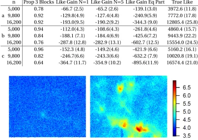
Table 2.3 Results from the unknown partition simulation that include proportion of

simulation iterates that correctly identified the partition to have 3 blocks, log likelihood gain as previously defined for 3 implementations of the stochastic

score estimation, and finally, the true log likelihood value 2 logL(θ,Y₀), where

the true simulation parameter settingsθand partition are used. . . 25

Table 2.4 Estimated mean and covariance parameters in the data analysis. . . 27

Table 3.1 Ordering Simulation. Average Rand Index for 100 samples for fixed p-value

cutoff 0.001 for partition setting a. with equally spaced base partitions. Paren-theses represent simulation standard error. . . 34

Table 3.2 Mean and standard error of the Rand Index for recovery of partitions for

com-parison of various base partition methods. . . 42

Table 3.3 Median number of stationary blocks estimated in various base partition

gen-eration methods in the gridded case. . . 43

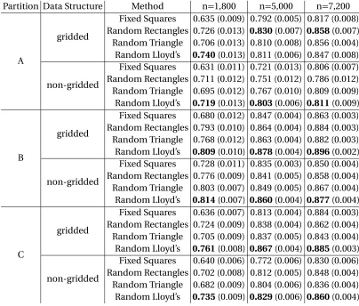
Table 3.4 MARDE for comparison of estimation of the evolutionary spectrum model on

full gridded data. . . 44

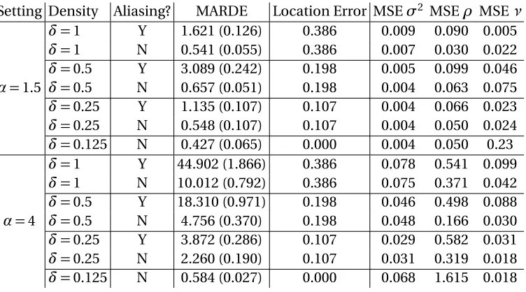
Table 3.5 Performance of estimated parameters when approximating various analysis

grid resolutions to the data with stationary covariance with spectral density

the square of Equation 3.7 whereσ2=1 andν=0.5. . . 46

Table 3.6 Results of 5-fold cross validation for various grid approximations to the data.

Note results are not comparable across resolutions because they utilize differ-ent datasets, and the folds are assigned individually. . . 49

Table 4.1 AIC values for testing model assumptions of pre-edge and post-edge

normal-ization regression estimates. Models are special cases of Equation 4.1. Bolded values are the best model in the case of each edge range. . . 59

Table 4.2 Median simulation root mean squared error (RMSE) and its simulation

stan-dard error of normalized spectra versus true simulated normalized spectra. . . 65

Table 4.3 Average simulation root mean squared error (RMSE) of spatial regression

coef-ficients. Simulation standard errors of the mean estimate are in parentheses. The minimum value in each error case is bolded. . . 70

Table 4.4 Chosen best fitting standard spectra via various methods with sample mean

and standard deviation over the 10×10 micron region. See Section 4.5.2 for

definitions of the fitting methods. . . 70

(10)

(11)

LIST OF FIGURES

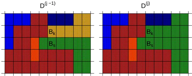
Figure 2.1 Example of block joining step ofBkandBsat thejt hstep of the partition

selec-tion algorithm assuming we cannot rejectH₀. Color represents membership

of the block to a partition segmentDi. . . 12

Figure 2.2 Absolute error in estimating the score using the independent and dependent

vector generation schemes. The dotted lines represent 95% prediction inter-vals for the absolute error in score estimation using 100 iterations at each sample size. The total sample size for the simulation was 400. . . 13

Figure 2.3 Sample draws from non-stationary models with increasingly non-stationary

parameter settings. We use these parameter settings for simulations in Section 2.5. . . 15

Figure 2.4 Mean likelihood gain under non-stationary settings (a,b,c) in comparison to

Vecchia likelihood approximation The shaded regions represent 95% point-wise confidence intervals in simulation. . . 20

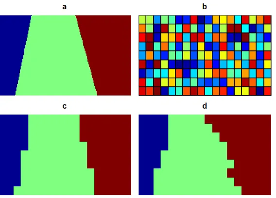
Figure 2.5 a. True partition, b. base partition, c. best possible partition with assumed

base structure (Rand=0.96), d. minimum BIC partition from simulation for

setting 3c (Rand=0.92). . . 22

Figure 2.6 Each plot shows Rand Indexes and BICs of one simulation of partition

estima-tion for sample size (1,2,3) and non-staestima-tionary setting (a,b,c). All regression lines are statistically significant. Red point indicates the chosen partition in each case. . . 23

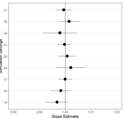
Figure 2.7 Each plot shows simulation mean slope estimate and 95% confidence

inter-vals for sample size (1,2,3) and non-stationary setting (a,b,c). All interinter-vals contain the true slope parameter 1. . . 24

Figure 2.8 Box plot of Rand indexes for sample sizes (1,2,3) and non-stationary settings

(a,b,c). The blue line represents the maximum possible Rand index given the base partition for the largest sample size (3), and the black line represents the equivalent Rand index for equal block division. . . 24

Figure 2.9 Arsenic fluorescence before (left) and after (right) lab treatment. . . 25

Figure 2.10 a. Log iron fluorescence before treatment, b. log Arsenic fluorescence after treatment, c. residuals of linear fit of simple linear regression of a. and b., d. scatter plot of a. and b. . . 26 Figure 2.11 a. Log arsenic distribution, b. spatial residuals recovered a different regression

in each block, c. selected partition structure for analysis (with color scheme that matches the subsequent plots), d. maximized parameter estimates of mean influence of log iron on log arsenic, e. maximized local variograms, and f. maximized local correlation functions. . . 28

Figure 3.1 Realizations from non-stationary models using the partitioning structure in

a. for traditional locally stationary models like Fuentes (2001) (b.) and the evolutionary spectrum model (c.). . . 32

Figure 3.2 Assumed partition structure and sample draws from each model used in

(12)

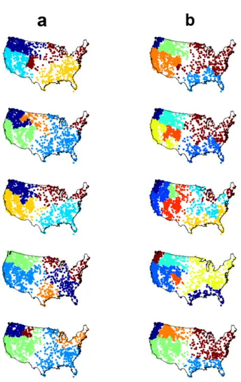
Figure 3.3 Examples of randomly generated base partitions (left) by equal partitioning, k-d tree generation, Delaunay triangularization, and Lloyd’s algorithm. Ex-amples of selected candidate partitions for non-stationary setting B (right), that have the Rand Indexes 0.846, 0.865, 0.861, and 0.877 respectively. . . 40

Figure 3.4 Assignment of point to resolutionsδ=1.0 (yellow),δ=0.5 (red), andδ=0.25

(blue). Black point (grid densityδ=0.125) is approximated to the colored

point in each resolution case, where all point within the colored box would be approximated to that same colored point. . . 45

Figure 3.5 Average daily temperature on the 2nd of each labeled month for 2018 at

mon-itoring locations. Data are sourced through the Global Historical Climatology Network Daily (GHCN-D). . . 47

Figure 3.6 Partition assignments for the 5-fold cross validation for low resolution 72×114

in a. and high resolution 144×225 in b. . . 48

Figure 3.7 Best candidate partition for second day in each labeled month in 2018 using

all monitoring stations. . . 50

Figure 3.8 Average daily temperature predictions for second day of each month using

our non-stationary model. . . 51

Figure 3.9 Results of analysis of average daily temperature on February 2, 2018. a. Data

approximated to high resolution grid, b. example random base partition corresponding to c, c. selected partition, d. predictions, e. marginal prediction

covariance, f. variograms of estimated local processes where distance is_40,0001

equal area grid unit. . . 51

Figure 4.1 Structure of unnormalized XANES stack data. 10×10 micron mapped region

with full XANES spectrum at each spatial location. Plotted spectra (left) is at the indicated spatial location on the map (right). The spatial map is shown at

energy=11990.25 eV. . . 55

Figure 4.2 Correlation of unnormalized spectra organized by distance of the spectra.

Smoothed spline is in red. . . 56

Figure 4.3 Normalized standard spectra considered in simulation and analysis. . . 57

Figure 4.4 Plot of collected unnormalized arsenic spectra. The indicated blue range is

the range of values used for pre-edge normalization and the indicated red range is the range of values used for post-edge normalization estimation. Energy is in eV. . . 58

Figure 4.5 First 9 possible basis components for assumed spatial structure to compose

spatially varying coefficients. Eigenvectors of eigendecomposition of Matérn covariance with scale 1, range 10, and smoothness 5. . . 61

Figure 4.6 Examples of simulated spectra under lowest and highest noise settings. . . 64

Figure 4.7 a. Simulation proportion of correctly identified standards, and b. proportion

of iterates where at least 2 standards were correctly identified. Definitions of legend abbreviations can be seen in Section 4.5.2. . . 67

Figure 4.8 Example of estimated spatially varying coefficients ( ˆβ) for each method in

one simulation setting whereσ=0.2. a. Truth, b. FI/PI, c. CF, d. SC, e. SU. . . . 68

Figure 4.9 Normalization of real data using independent normalization (left) and spatial

(13)

Figure 4.10 Estimated proportion contribution for the spatially constrained analysis (SC) for the following standards: a. scorodite, b. calcium-arsenate, and c. As(III)-Fe-peat. . . 69 Figure 4.11 Normalization comparison for a subset of spectra for independent

normal-ization (black) vs. our spatial normalnormal-ization (red). . . 71 Figure 4.12 Examples of spectra fittings for our spatially constrained fitting procedure. . . 72

Figure A.1 Results of analysis of daily average temperature on April 2, 2018. a. Data

Figure A.2 Results of analysis of daily average temperature on October 2, 2018. a. Data

Figure A.3 Results of analysis of daily average temperature on December 2, 2018. a.

Data approximated to high resolution grid, b. example random base partition corresponding to c, c. selected partition, d. predictions, e. marginal prediction

(14)

CHAPTER

1 INTRODUCTION

Gaussian process models are useful tools in answering numerous modern scientific questions.

Unlike regression models where the observations are assumed to be independent and identically distributed, Gaussian process regression models can account for correlation among observations.

In accounting for this correlation, uncertainties associated with mean parameters estimates are

more accurately characterized. Additionally, prediction or kriging is a natural application of these models.

This modeling is particularly useful in the case where observations are collected over space or

time. Correlation of these observations are ordered so that observations closer in space or time are naturally more correlated than those at distant locations. For example, the temperature in Raleigh,

NC is closely related to the temperature in Durham, NC because they are close in space. However,

both are less correlated with the temperature in Cincinnati, Ohio due to distance and other factors associated with distance. These models are further helpful in applications such as computer model

emulation where the domain of interest is parameter space rather than physical space (Conti et al.

2009). In this dissertation, we study Gaussian process models for data collected over space, and therefore the following definitions will be described in this case. However, this work is potentially

generalizable to other applications.

Formally, defining a Gaussian process induces a jointly normal multivariate distribution between

any data collected on the continuous spatial domain. Assume that we observe data at spatial

(15)

at those spatial locationsY = (Y(s1),Y(s2), ...,Y(sn))T, andX be then×(p+1)design matrix that

containsp covariates observed at those locations. Thenβis the(p+1)×1 vector of unknown mean

parameters. Typical parametric Gaussian process regression models define the covariance between

points as a parametric formK(θ). Then the loglikelihoodL(θ)of the dataY is

l o g(L(θ)) =−n

2l o g(2π)−

1

2l o g(|K(θ)|)−

1

2(Y −Xβ)

T_K₍_θ₎−1₍_Y ₋_X_β₎_. _(1.1)

Often this covarianceK(θ)is assumed to be isotropic and stationary. In spatial statistics, this means

that the correlation of points is determined only by the Euclidean distance between them. Formally,

the stationary covariance between spatial locationss1ands2is defined as

K(s1,s2) =φ(θ,||s1−s2||), (1.2)

for some continuous functionφ:[0,∞)→Rcontrolled by parametersθ. Common choices of

covariance structures include the flexible Matérn covariance, exponential covariance, and

squared-exponential forms. We typically need to evaluate the log likelihood many times to estimate

parame-tersθ. However, when data are large and collected on diverse environmental domains, this analysis

becomes problematic.

First, since the domains are large and defined over heterogeneous environmental conditions, the assumption of stationarity is potentially unrealistic. Further, if dense covariance matrices are

defined, memory limits often prohibit the formation of the covariance matrix when the datasets

are large (>10,000). Therefore, defining such models and developing methods in which to compute

corresponding parameter estimates is an area of active research (Heaton et al. 2018).

Models can account for stationarity in the mean, covariance, or both. In first order

non-stationary models, the mean is assumed to be spatially varying with respect to the covariates. Formally they are defined as

Y(s) =X(s)β(s) +ε(s), (1.3)

whereε∼G P(0,K). Then , the mean contributions of the covariates is dependent on spatial location.

Typically, theβ(s)are constrained or further defined so that there is a smooth structure on the way in which the estimates are allowed to vary over space.

A simple set of constraints in spatially varying coefficients can be defined through spatial interaction effects. Imagine we observe data over euclidean space so thats = (x,y)∈R2. Then the spatially varying

coefficients that are as linearly changing over the domain can be written as

(16)

whereb0,b1,b2,b3are unknown mean coefficients. Other polynomial trends can be substituted to increase

the complexity of the spatially varying structure in such a model. These models are very easy to understand, but are very limiting, and it is rarely the case that such simple interactions model observational data well.

Spatially varying coefficients can also be constrained so that the data are divided into a partitionP=

{P1,P2, ...PQ}. Then, a linear model is fit independently for each block of the partition. This can formally be written withIas an indicator function as

β(s) =

Q

X

i=1

I{s∈Pi}bi, (1.5)

wherebi fori =1, 2, ...,Q are unknown mean coefficients. This model is very useful, and in fact, has a similar foundational concept to that of the machine learning technique of decision trees (applicable to random forests), where data are partitioned in parameter space rather than physical space (Liaw & Wiener 2002). However, predictions from this model are non-smooth across the definitions of the blocks and those definitions are not always easy to define.

A popular spatially varying coefficients model introduces the spatial smoothness through spatially smooth basis functions. In these models, each spatially varying parameterβi(s)is decomposed into the linear combination of fixed basis functionsqi(s)wherei=1, 2, ...,was

βi(s) =b0+b1q1(s) +...+bwqw(s), (1.6) wherebi fori =0, 1, ...,w are unknown mean coefficients. These spatially smooth basis functions can be generated via any number of methods, but radial basis functions and eigenvector decompositions are popular choices.Eigenvector spatial filtering (ESF) is one such method (Griffith 2013). In this case, the eigendecompo-sition of a covariance matrix is performed and the firstweigenvectors are used as the fixed effectsqi(s). These models are flexible, and increasingly smooth spatial constraints can be imposed with smallerw. However, there is no one universally best selection criterion for the number of componentsw.

Finally, the most complex common version of spatially varying coefficient models includes assuming that the mean parametersβ(s)follow a Gaussian process (Gelfand et al. 2003). This is most easily estimated in the case of Bayesian statistics using MCMC. This flexible, but is more difficult to estimate, especially in the case of a large number of location. IfK =σ2_I_{, estimating this model is equivalent to estimating a spatially}

correlated Gaussian process regression model with a nugget parameter.

(17)

The Haas (1995) moving window model is applicable to modern large environmental data as in Kuusela & Stein (2018). In this model, data at each spatial location is modeled using only data within a predetermined window surrounding that point. However, the influence of the size and shape of the analysis window is not well studied. This model is convenient because it can easily be parallelized, but this means that there is no overall coherent interpretable model.

As alternate means of parameter estimation, there have been a series of likelihood approximations to the multivariate normal likelihood applicable to multiple covariance structures. The most popular of these is the Vecchia Likelihood approximation (Vecchia 1988), which is similar to the nearest neighbor Gaussian process (NNGP) (Datta et al. 2016). In these approximations, the conditional representation of the likelihood is approximated by only including the nearest points in the conditioning set. Further work such as Katzfuss & Guinness (2017) have increased the accuracy of these methods generalizing the framework for Gaussian process approximations. The Whittle Likelihood (Whittle 1954) is another popular approximation. Here, the covariance matrix is assumed to be circulant so that an application the FFT (fast Fourier transform) diagonalizes the covariance matrix into a spectral density. This assumption is typically assuaged through tapering the edges of the data referred to as buffering. Since the circulant assumption is vital to computational efficiency, this method is only applicable to data on grids with no missing data. Finally, covariance tapering is also a popular approximation technique. In this method, the covariance matrix is pointwise multiplied by a tapering matrix to induce sparsity (Stein 2012). In the case where only the covariance matrix is tapered (one-taper) the estimates of the covariance parameters are biased (Kaufman et al. 2008). However, when a taper is also added to the empirical covariance (two-taper), the covariance parameters can be estimated unbiasedly at the cost of computational efficiency (Kaufman et al. 2008). This approximation is also not studied in the case of non-stationary models.

In this dissertation, we focus on the advancement of computation of a special case of locally stationary models. We partition the domain so that within each block, the data follows a stationary Gaussian process model. One type of these models were popularized by Fuentes (2001) and have more recently been expanded on by Risser et al. (2016). In these works, a non-stationary Gaussian process is modeled as the spatially varying weighted sum of stationary Gaussian processes. A drawback of these models is that they have discontinuities in the covariance and the predictions along block divisions or employ computationally intensive model-averaging to avoid these. In Fuentes’ implementation of this model, the data are divided into equally-sized blocks and analyzed individually. Risser et al. (2016) use a partitioned model for non-stationary data, but use the covariate information to define the boundaries. In both cases, these blocks must be small enough so that the maximum likelihood parameters can be estimated directly through formation of the covariance matrix, or they must be non missing grids rectangular in shape so that spectral methods such as the Whittle likelihood can be implemented.

(18)

In this dissertation, we develop computational methodology to these non-stationary models. Our compu-tational methods first estimate locally stationary partitions of the domain. Further, we develop a parameter estimation algorithm that utilizes stochastic score approximations Stein et al. (2013) and exploits gridded data structure for fast parameter estimation inO(n)storage andO(nlog(n))computation per iteration.

1.1 Stochastic Score Approximation

Stein et al. (2013) propose stochastic score approximations to estimate parameters in stationary Gaussian process models without formation of the covariance matrix. Letθ= (θ1, . . . ,θq)be a vector of the covariance parameters andK(θ)be the covariance of the multivariate normal likelihood withY0as then×1 data vector

with mean trend removed. We consider a mean linear in the covariates soY0(s) =Y(s)−X(s)βˆG LS. where ˆ

βG LS= (XTK−1(θ)X)−1XTK−1(θ)Y. Then the score of the multivariate normal log likelihoodL(θ,Y0)is ∂

∂ θi

L(θ,Y0) =S(θi|Y0) =

1 2Y

T

0 K− 1₍_θ₎_K

i(θ)K−1(θ)Y0−

1 2t r(K

−1₍_θ₎_K

i(θ)), (1.7)

whereKi(θ) =∂ θ∂iK(θ). Evaluation of the trace term requires either formation of ann×nmatrix ornlinear

solves. This is inefficient since the score function will need to be evaluated repeatedly to estimate parameters using maximum likelihood estimation.

By using the Hutchinson (1990) trace approximation, Stein et al. (2013) approximate the score of the multivariate normal log likelihood by

S(θi|Y0)≈Se(θ_i|Y₀) =

1 2Y

T

0 K− 1₍_θ₎_K

i(θ)K−1(θ)Y0−

1 2N

N

X

j=1

U_jTK−1(θ)Ki(θ)Uj, (1.8) where elementkof then×1 vectorU1is sampled so thatUj k∼Bernoulli(p=12; 1,−1). The remainingUj vectors are constructed from a dependent sampling scheme so that the expected value of the score is zero andSe(θ_i|Y₀)fori=1, ...qis a set of unbiased estimation equations. Using orthogonal vectors ensures that the

trace approximation converges to the true trace asNapproachesn.

Stein et al. (2013) show this formulation is convenient computationally in the stationary case through avoidance of formation of the covariance matrix directly by circulant embedding. In the case of gridded data and stationary covarianceK(θ), circulant embedding can perform matrix-vector multiplication inO(nlog(n)) computation andO(n)storage (Dietrich & Newsam 1997). By applying the Fast Fourier Transform (FFT) to a circulant matrix, it is diagonalized. This theory is applied so that a stationary covariance matrix on an expanded domain is reduced to its spectral density. Guinness & Fuentes (2017) show this procedure works well even with relatively small expansion factors such as5₄. We extend this work in this dissertation by generalizing these tools to non-stationary models. Thus, we are able to evaluate an unbiased approximation of the score inO(n)storage andO(nlog(n))operations as compared toO(n2₎_{storage and}_O₍_n3₎_{operations of computing}

the likelihood directly for two full-rank, non-stationary covariance matrices.

By computing the Fisher information matrix forθ, the asymptotic variance of the maximum likelihood parameters in the multivariate normal are1₂t r(K−1₍_θ₎_K

(19)

al (2013), they derive that thei,j element of the information matrixBof estimates obtained via stochastic score have elements:

Bi,j= ( 1 2+

1 2N)t r(K

−1₍_θ₎_K

i(θ)K−1(θ)Kj(θ))− 1

2Nt r((KiK

−1₎_∗₍_K

jK−1)), (1.9) where∗is element-wise multiplication. In this formulation, we observe a few properties of the approximation. First, asN → ∞, the asymptotic variance of the estimates approaches that of the traditional maximum likelihood estimation. Additionally, the variance of the approximation does vary by the function of the parameter and therefore parameters with large maximum likelihood variances, will also have higher variance induced by use of the stochastic score. This dissertation will extend these stochastic score approximations for the estimation of parameters in locally stationary models.

1.2 Scientific Motivation of Research

Non-stationary models are widely applicable to numerous environmental applications. In Chapters 2 and 4, we apply first and second order non-stationary models to further understand the mechanisms of arsenic binding in soils. Arsenic in drinking water, even in trace amounts, can be extremely harmful to human health with prolonged exposure (Council 1999, Brown & Ross 2002). In many parts of the world where there is not access to filtered, clean drinking water, arsenic poisoning is an extreme danger (Nordstrom 2002). Whether arsenic is sourced naturally, through mining and agricultural practices, or other man-made sources, it becomes harmful when it is dissolved into groundwater through wells and other aquifer sources. This contaminates the environment and harms human health (Smith et al. 2002). Thus, it is of vital scientific interest to understand what soil components bind to arsenic so that we may strengthen the bindings or design filters to purify the water. It is well known how arsenic should bind in pure systems through chemical formulas, but in the complex and heterogeneous conditions of soil, the proclivities and diversity of its binding mechanisms are not well understood. Current technologies such as synchrotron X-Ray fluorescence microprobe (XRF) and X-Ray absorption near edge structure (XANES) spectroscopy allow for the examination of the sub-micron binding of arsenic and to characterize its variation on an arsenic-treated sand grain.

In Chapter 3, we model average daily temperatures. Temperature is an important environmental variable that is of primary interest to track the progress of climate change (Folland et al. 2001). Additionally, tempera-ture, particularly extreme temperatures, can determine human and environmental health (McMichael et al. 2006). Finally, temperature is needed in many numerical models in order to simulate or predict other envi-ronmental variables of interest (Byun & Schere 2006). We utilize the new computational methods developed in this dissertation in order to more accurately predict average temperature on a fine grid.

1.3 Preview of Chapters

(20)

in its practical use is in the definition of the boundaries for the local processes, and therefore we describe one such selection procedure that generally captures complex non-stationary relationships. We generalize the use of stochastic approximation to the score equations for data on a partial grid in this non-stationary case and provide tools for evaluating the approximate score inO(nlogn)operations andO(n)storage. We perform various simulations to explore the effectiveness and speed of the proposed methods and conclude by making inference on the accumulation behavior of arsenic applied to a sand grain.

In Chapter 3, we further extend the methods presented in Chapter 2 in order to generalize the use of a different non-stationary model. Here, we utilize the evolutionary spectrum model, which had previously only been computationally applicable to square non-missing gridded data. We hone our partition selection algorithm particularly by considering randomly generated base partitions that lead to more flexible partition candidates. Although our parameter estimation methods are still developed in the case of partially gridded data using the stochastic score, we test the applicability of them to irregularly spaced data by approximating a fine grid. Here we apply our methods to average temperature for 12 days in 2018 at irregularly spaced monitoring locations in order to predict temperature at finely gridded locations across the US.

(21)

CHAPTER

2 NON-STATIONARY COVARIANCE

ESTIMATION USING THE STOCHASTIC

SCORE FOR LARGE SPATIAL DATA

2.1 Introduction

Large environmental datasets are often defined on naturally heterogeneous fields or have other inherently spatially varying conditions. Therefore, it is unreasonable to expect a response variable to be well-modeled by a stationary process over a large domain space. However, using non-stationary models is difficult in practice due to the conceptual challenges in specifying the model and the computational challenges of fitting the model when the data are so large that memory constraints prevent formation of the covariance matrix. We propose a simple, but flexible parametric non-stationary model and corresponding computationally efficient statistical methods for estimating the model from large datasets.

Our modeling approach is similar to that in Fuentes (2001,2002), but our estimation method differs and allows us to extend its practical implementation. Fuentes models the non-stationary processY(s)at spatial locationsas locally-stationary processes:

Y(s) =

q

X

i=0

ωi(s)Zi(s), (2.1)

(22)

form of a covariance function. The covariance function ofZiis specified parametrically with parametersθi, and inference onθiis the primary goal of estimation. Theωi are assumed to be non-random, unknown, and positive spatially contiguous weights. Although the model specification allows the weighting functionsωito be quite general functions, in this paper we assume the weighting functions form a partition of the domain in order to capture non-smooth changes in the covariance. Our parameter estimation method, however, is more broadly applicable to the model and is not limited to this simplification. We formally define partitioning the domainD by{D₁, . . . ,Dq}such thatD=∪qi=1Di. Lets ∈Dand fori=1, 2, ...,q,ωi(s) =1 ifs∈Di and 0 otherwise. Letω0(s) =1 for all spatial locationss.

This particular formulation of the model has many application-driven advantages. First, its structure (ω) has an intuitive and scientifically flexible design. For example, there may be scientifically relevant reasons to partition the field in a certain way or specific known features that are expected to influence the correlation structure of certain points. For example, in spatial data across the United States, the partition structure could be defined along state lines in order for analysis to inform policy decisions. However in the application considered in this paper, we do not have a priori knowledge of a partition for analysis. Next, the model lends itself to well-known testing and model selection procedures. Likelihood ratio tests could be performed to explore null hypotheses about the Gaussian processes in order to interpret the parameters and how they change across the field. Finally, familiar choices of covariance structures can continue to be used and interpreted as such.

In Fuentes’ implementation of this model, computational necessity drives its practical application. Some adjacent points are assumed independent so that the data are divided into equally sized blocks and analyzed individually. Similarly, Risser et al. (2016) use a partitioned model for non-stationary data, but use the covariate information to define the boundaries. In both cases, these blocks must be small enough so that the maximum likelihood parameters can be estimated directly through formation of the covariance matrix, or they must be rectangular in shape so that spectral methods such as the Whittle likelihood can be implemented. Our method of estimation relaxes these assumptions by allowing partition blocks of any size and shape as chosen by the data-driven procedure introduced in Section 2.2. Additionally, our model generalizes the practical application of Fuentes’ model by definingω1(s) =1. This defines globally stationary component that was

previously computationally difficult so that all points are potentially spatially correlated (Fuentes et al. 2007). Of importance to estimating the model well is the number of processesq and their accompanying structure, and we present a computationally efficient method to select this in Section 2.2. In Risser et al. (2016), they define blocks only through covariate information. We instead implement a method based on likelihood ratio testing that directly uses the estimated spatial correlation of the data to cluster the locations into spatially contiguous partition blocks. To overcome previous restrictions to the model to estimateµi,θi, we propose a new estimation method involving the generalization of Stein et al. (2013) stochastic score approximation to the non-stationary case. Our work describes the solving of non-linear systems with non-stationary covariances through unique application of circulant embedding, new preconditioners, and spectral density differentiation. Implementation details are provided for data in the gridded case and yield a corresponding new estimation method that is computationallyO(nlog(n))andO(n)memory.

(23)

selection method they present utilizes the Ising model to uncover stationary blocks of the domain. However, their estimation procedure depends on a determinant approximation that is not well understood, and since the Ising model relies on a fixed number of partition blocks, they must fully estimate parameters in several models to select a partition.

In kernel convolution (Higdon 1998), spatially-varying kernel functions are convolved with a station-ary, often white noise, process. The parameters of the model are defined in the kernel function, and they demonstrate the model’s benefits using Bayesian estimation.While this type of model is flexible, its practical implementation approximates the convolution integral with a small number of components, which leads to a low-rank covariance matrix. Our method requires no rank reduction of the covariance matrix in order to be computed quickly.

Other classical non-stationary models have been well-studied. Deformation models require the formation of full covariance matrices and are therefore computationally inefficient for large datasets (Sampson & Guttorp 1992). Moving windows (Haas 1995) have been proposed to estimate non-stationary covariances. However, since it involves defining the covariance with a moving window of the data, there is no guarantee that the resulting global model covariance is positive definite or can even be fully defined.

The environmental application we consider is in micro-scale soil science. When trace amounts of arsenic are dispersed into the environment, it can be harmful to life through contamination of water, plants, and soil. Although the theoretical chemical binding of pure arsenic is well understood, it is not clear how it will chemically bind in the heterogeneous conditions of the soil, where both organic matter and minerals coexist in diverse spatial patterns. By studying the micro-scale accumulation behavior of arsenic applied to a sand grain, we can characterize how its spatial correlation is impacted by its association with soil components. Studying this gives us insight to potential lurking variables that can describe arsenic’s preference to bind beyond elemental structure. However, since there is diverse spatial heterogeneity of the multi-element composition across a 100×100 micron region, we expect the spatial correlation to vary with space. Thus, our objective is to better understand the diversity of micro-scale spatial correlation of the accumulation of arsenic on a sand grain.

In Section 2.2, we describe a new method for estimating the partition structure of theω, and then in Section 2.3 we generalize the use stochastic approximation to the score function to the non-stationary case and detail other computational tools involving the FFT for fast score computation for gridded data. Next in Section 2.4, we describe an algorithm to estimate the parameters quickly. In Section 2.5, we perform simulation studies to numerically validate the estimation method, and finally in Section 3.6, we apply our method in order to draw scientific conclusions.

2.2 Partition Estimation Method

(24)

(2001) the partition structure is chosen via BIC from an ensemble of candidates of only equally sized blocks. This structure is not likely in natural systems so we propose a method that self-selects shape and size of the partition blocks through likelihood ratio testing.

To estimate one partition candidate, we begin by partitioning the domain into a base partitionB. This partition is made ofq(0)_{equally spaced blocks so that}_B₌_{_B

1,B2, ...Bq(0)}.Bis chosen by the modeler, and we chose square blocks of 10×10 pixels as seen in Figure 2.1, though other choices are possible. Our method for generating a partitionDis iterative and is initialized withD(0)₌_B_{so that}_D(0)

i =Bi. At stepj+1 of the partition selection algorithm, the partitionD(j+1)_{is formed by possibly joining two neighboring blocks of} the partitionD(j)_{, according to a likelihood ratio test to be described below. This means that any block}_D(j) i consists of a subset of{B1, . . . ,Bq(0)}. Partitions define an equivalence relation, in the sense thati(

j)

∼kifBiand

Bk are both in the same block ofD(j). Letθi be a lengthpvector of covariance parameters describing block

Bi and wheni (j)

∼k,θi=θk.

Define the setNBof all pairs of neighbor blocksNB={{Bs,Bk}|BsneighborsBk}withnBelements. Then at the(j+1)th step of the algorithm, we randomly sample one pair{Bs,Bk}fromNBtest the hypothesis:

H0:θs=θk, (2.2)

H1:θs6=θk, (2.3)

with a likelihood ratio test statisticΛ(Bs,Bk|D(j))defined below. Assume for illustration thatBs∈Ds(j)and

Bk∈D( j)

k . If we cannot rejectH0, we join the blocks settingD(

j+1) s =D(

j) s ∪D(

j) k andD

(j+1)

k =;. However, if we rejectH0, all values are unchanged in the update so thatD(j+1)=D(j).

The likelihood ratio test is based on the test statistic:

Λ(Bs,Bk|D(j)) =

Q

i(j)∼s,i(j)∼k

L(θ˜(j+1)_|_B i)

Q

g(∼j)s

L(θˆg(j)|Bg)

Q

h(∼j)k

L(θˆ_h(j)|Bh)

, (2.4)

where ˜θ(j+1)_{be the maximized parameter values such that}_H

0is true at stagej+1 for the likelihood

Q

g(j)∼s

L(θg|Bg)

Q

h(j)∼k

L(θh|Bh)and ˆθi(j)is the maximized parameter values for blockBi at the stagej. We compare

−2l o g(Λ)to theχ2

pdistribution to obtain a p-value for the test. This is compared to a small p-value cutoff that anticipates increased type I errors from multiplicity, and the appropriate action is made to obtainD(j+1)_.

We continue to sample neighbor pairs fromNB without replacement exhaustively. The final state of the partitionD(nB)_{gives a candidate partition structure. The candidate depends on the significance level}

chosen for the likelihood ratio testing as well as the random sampling of the neighbor pairs. Thus, we suggest trying a variety of small p-value cutoffs and repeating this procedure to obtain a set ofl viable partitions

{P1_,_P2_{, ...,}_Pl_}_{. Let ˆ}_θm_{be the vector of all maximized covariance parameters describing partition}_Pm_and ˆ

θm