The Rossiter-McLaughlin effect for exoplanets
J.N. Winn
Department of Physics, and Kavli Institute for Astrophysics and Space Research, Massachusetts Institute of Technology [[email protected]]
Abstract. There are now more than 30 stars with transiting planets for which the stellar obliquity—or more precisely its sky projection—has been measured, via the eponymous effect of Rossiter and McLaughlin. The history of these measurements is intriguing. For 8 years a case was gradually building that the orbits of hot Jupiters are always well-aligned with the rotation of their parent stars. Then in a sudden reversal, many misaligned systems were found, and it now seems that even retrograde systems are not uncommon. I review the measurement technique underlying these discoveries, the patterns that have emerged from the data, and the implications for theories of planet formation and migration.
1. Introduction
When was the first announcement of the detection of a planetary transit? About 10 years ago, the transits of HD 209458b were reported by two different groups (Henry et al. 2000, Charbonneau et al. 2000). However, planetary transits have a much longer history. A transit of Venus was first witnessed in 1639, by Jeremiah Horrocks. And even before that, in 1611, Christoph Scheiner reported the detection of a system of close-in planets transiting the Sun (see, e.g., Casanova 1997).
Scheiner was wrong, and was eventually convinced he was seeing dark spots in the Sun’s atmosphere, rather than transiting planets. He then charted the trajectories of sunspots over the years, and thereby discovered that the Sun’s equatorial plane is not perfectly aligned with the plane of Earth’s orbit: the solar obliquity is about 7◦
. Now that we know of many other stars harboring planets, it would be interest-ing to know whether this degree of alignment is common, or unusual. Even though planets are thought to have formed on well-aligned circular orbits, there are reasons to expect occasional misalignments. Many exoplanets are observed to have eccentric orbits, and whatever process excited their eccentricities may also have excited their inclinations. Furthermore, for close-in planets, there are various “migration” scenar-ios for bringing the planets inward from beyond the snow line, which make differing predictions about spin-orbit alignment. Migration through tidal interactions with a protoplanetary disk would damp any initial inclination (see, e.g., Marzari & Nelson 2009). In contrast, planet-planet scattering would amplify any initial inclinations (e.g., Chatterjee et al. 2008), and the Kozai effect due a companion star or distant planet can produce drastic misalignments (Fabrycky & Tremaine 2007).
Scheiner’s method cannot be used for exoplanets, at least not until our technology allows the disks of planet-hosting stars to be resolved. Instead, the stellar obliquity © Owned by the authors, published by EDP Sciences, 2011
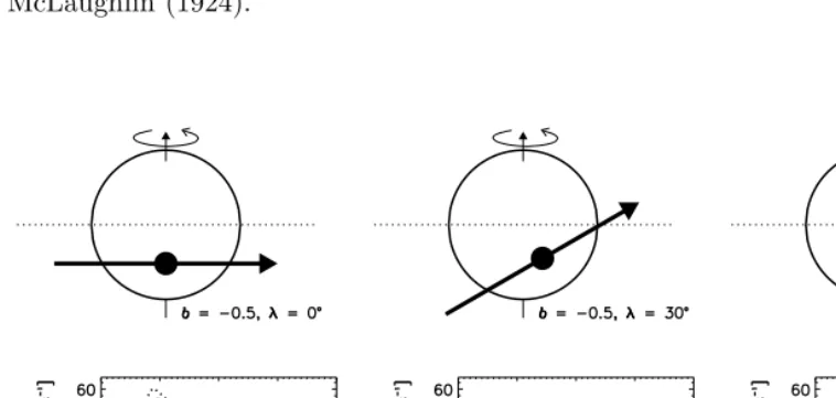
can be assessed by observing a phenomenon known as the Rossiter-McLaughlin (RM) effect. During a transit, part of the rotating stellar surface is hidden, weakening the corresponding velocity components of the stellar absorption lines. When the blueshifted (approaching) half of the star is blocked, the spectrum appears slightly redshifted. Likewise, when the redshifted (receding) half of the star is blocked, the spectrum is blueshifted. The result is an “anomalous Doppler shift” that varies throughout the eclipse (see Figures 1 and 2). By monitoring the stellar line profiles throughout eclipses, we can measure the angle between the sky projections of the orbital and spin axes. This phenomenon was first predicted by Holt (1893) and observed by Rossiter (1924) and McLaughlin (1924).
Figure 1: The RM effect as an anomalous Doppler shift. Top: three transit geometries that produce identical light curves, but differ in spin-orbit alignment. Bot-tom: corresponding radial-velocity signals. Good spin-orbit alignment (left) produces a
symmetric “redshift-then-blueshift” signal, a 30◦
tilt (middle) produces an asymmetric
signal, and a 60◦
tilt (right) produces a blueshift throughout the transit. From Gaudi & Winn (2007).
2. Observations of the RM effect
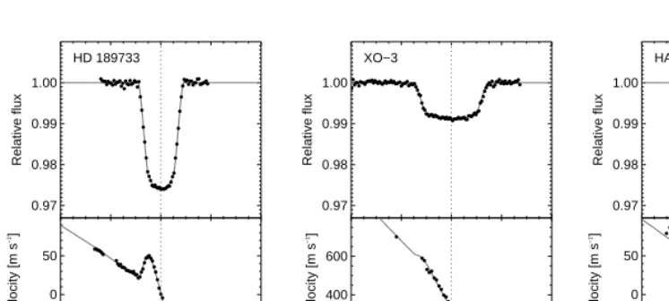
The exoplanetary RM effect was first detected by Queloz et al. (2000), who showed the orbit of the “hot Jupiter” HD 209458b is prograde. More recent measurements have revealed a diversity of orbits, including some that are very well-aligned with the equatorial planes of their parent stars, some that are misaligned by more than 30◦
, and even some that are apparently retrograde. Examples from each of these categories are shown in Figure 3.
Figure 2: The RM effect as a spectral distortion. Top: three successive phases of a transit. Middle and bottom panels: same, but showing the line-of-sight rotation velocity of the photosphere as a gradient, as well as the distorted spectral line profile. Middle: a low obliquity. The spectral distortion moves from the blue side to the red side. Bottom: a projected obliquity of 60◦. In this case the obscuration by the planet
0.97 0.98 0.99 1.00 Relative flux HD 189733
−4 −2 0 2 4
Time [hr] −100
−50 0 50
Radial velocity [m s
−1]
λ = −1.4˚ ± 1.1˚
0.97 0.98 0.99 1.00 Relative flux XO−3
−4 −2 0 2 4
Time [hr] 0
200 400 600
Radial velocity [m s
−1]
λ = 37.3˚ ± 3.7˚
0.97 0.98 0.99 1.00 Relative flux HAT−P−7
−4 −2 0 2 4
Time [hr] −100
−50 0 50
Radial velocity [m s
−1]
λ = 182.5˚ ± 9.4˚
Figure 3: Examples of RM data. The top panels show transit photometry, and the bottom panels show the apparent radial velocity of the star, including both orbital motion and the anomalous Doppler shift. The left panels show a well-aligned system, the middle panels show a misaligned system, and the right panels show a system for which the stellar and orbital “north poles” are nearly antiparallel on the sky. From Winn et al. (2006; 2009a,b).
the amazingly good fortune that the planet’s orbit is viewed close enough to edge-on to exhibit transits, and a large community effort to observe the photometric and spec-troscopic transits. H´ebrard et al. (2010) have performed the most definitive analysis.
Another important accomplishment was the measurement by Triaud et al. (2010) of the RM effect of six systems, half of which showed evidence for retrograde orbits. This suggested that misaligned orbits may be common, rather than exceptional, and increased the sample size by enough to allow meaningful searches for patterns among the properties of the stars, planets, and orbits.
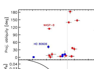
One possible pattern that has emerged is that stars with high obliquities are pref-erentially those with the highest effective temperatures (i.e. the most massive). This is illustrated in Figure 4. This finding could help to explain the otherwise puzzling history of RM observations: the first 10 published analyses were all consistent with good alignment, while the next 20 showed a much wider range of obliquities. The ex-planation could be that cooler stars were examined earlier, as they allow for better RV precision and greater ease of detecting planets. Indeed, most Doppler surveys exclude early-type stars altogether.
star, one could invoke core-envelope decoupling, but it is unclear why the coupling would be so weak and it is also not observed in the Sun. For further discussion, see Winn et al. (2010a).
Figure 4: Misaligned systems have hotter stars. Top: the projected obliquity is plotted against the effective temperature of the host star. A transition from mainly
aligned to mainly misaligned seems to occur atTeff ≈6250 K. The two strongest
excep-tions (labeled) are also the systems with the weakest expected tidal interacexcep-tions. Squares indicate systems discovered by RV surveys, while circles indicate systems found in pho-tometric transit surveys. Bottom: the mass of the convective zone of a main-sequence
star as a function ofTeff, from Pinsonneault et al. (2001). It is suggestive that 6250 K
is approximately the temperature at which the mass of the convective zone becomes negligible. From Winn et al. (2010a).
obliquities: it implicates tidal evolution as the reason for low obliquities among cool stars with more massive planets in tighter orbits (Winn et al. 2010a).
−4 −2 0 2 4
Time since midtransit [hours] −10
0 10
Anomalous RV + const [m s
−1]
May 26/27
Both transits (binned)
Aug 22/23
−10 0 10
RV [m s
−1]
−2 −1 0 1 2
Time since midtransit [days] −10
0 10
O−C [m s
−1]
Figure 5: The RM effect for the “super-Neptune” HAT-P-11. Left: spectro-scopic orbit of HAT-P-11. Right: anomalous RV of HAT-P-11 spanning two transits (top and bottom), and the time-binned combination (middle; binned 7 with a maximum bin size of 0.5 hr). The second transit was observed during the OHP meeting. The solid line shows the best-fitting model of the RM effect. The dashed curve shows the
best-fitting “well-aligned” model (λ= 0, vsini= 1.3 km s−1
), which is ruled out with
∆χ2= 52.4. From Winn et al. (2010c).
In addition, Schlaufman (2010) presented evidence that hot stars have high obliq-uities, based on a completely different technique. His idea was to compare the vsini distribution of stars with transiting planets with those of random stars of the same mass and evolutionary state. To the extent that the transit stars have rotation axies parallel to the orbital axes, they will have systematically largervsinivalues than their non-transited brethren, because sini= 1 for the eclipsing systems while 0 <sini <1 for random stars. As shown in Figure 8, he found that more massive stars have higher obliquities than lower-mass stars, with the transition at around 1.2M⊙, consistent with
the transition temperature ofTeff = 6250 K found by Winn et al. (2010a).
3. Implications for planet migration
0.0 0.5 1.0 1.5
−20
−15
−10
−5
0
5
10
Stellar
Mass
[
M
Sun]
R
o
ta
ti
o
n
S
ta
ti
st
ic
Θ
Mp≥3JupiterMass
Mp=2JupiterMass
Mp=1JupiterMass
Mp≤0.1JupiterMass
SPOCS Control Sample
a
[
AU
]
0 0.01 0.02 0.03 0.04 0.05 0.06 0.07 0.08 0.09 0.1
(Triaud et al. 2010, Winn et al. 2010a, Matsumura et al. 2010). To appreciate the strengths and weaknesses of this argument, it is useful to frame it as a series of premises:
1. Hot Jupiters formed beyond the snow line and migrated inward.
2. The orbit and spin were initially aligned.
3. The two migration theories are disk-planet interactions and few-body dynamics.
– Disk-planet interactions damp inclinations. – Few-body dynamics excite inclinations.1
– Nothing else excites inclinations.
4. Many hot Jupiters have high inclinations.
From these premises it follows that the misaligned hot Jupiters migrated via few-body dynamics. Furthermore, it is possible that allhot Jupiters migrated this way, if tides are responsible for the low observed inclinations.
Some authors have already challenged these premises. For example, it is possible that protoplanetary disks are frequently misaligned with the rotation of their host stars (Bate, Lodato, & Pringle 2010; Lai, Foucart, & Lin 2010). In addition, we heard at this meeting from C. Moutou that the spin orientation of stars may tumble chaotically due to a fluid instability. Tests of these ideas are possible with RM observations of multiple-planet systems (Fabrycky 2009, Ragozzine & Holman 2010), and of binary stars (Albrecht et al. 2009, 2010).
It is important to remember that this argument focuses exclusively on hot Jupiters. Disk migration has become vulnerable as an explanation for those planets, but is still viable (and without a good alternative) for explaining the “medium-period” giant plan-ets, well within the snow line but too distant for tidal effects to be important. The mean-motion resonances that are occasionally observed among such planets are evi-dence for disk migration. The priority for future observations of the RM effect is to explore a more diverse sample of planets, including rocky planets, long-period planets, and multiple-planet systems.
Acknowledgements. I am grateful to the local organizing committee, for organizing a productive
and memorable meeting. I thank Simon Albrecht for comments on the draft of this contribution, and Kevin Schlaufman for providing Figure 6. Finally, I extend my gratitude to the colleagues with whom I have worked closely on this topic: Yasushi Suto, Ed Turner, Geoff Marcy, Bob Noyes, John Johnson, Norio Narita, Dan Fabrycky, Andrew Howard, and Simon Albrecht.
References
Albrecht et al. 2009, Nature, 461, 373
Albrecht et al. 2010, ApJ, in press [arxiv:1011.0425] Anderson et al. 2010, ApJ, 709, 159
Bate, Lodato, & Pringle 2010, MNRAS, 401, 1505 Bayliss et al. 2010, ApJL, 722, 224
1“Few-body dynamics” is meant here to include some combination of planet-planet interactions and the
Casanova 1997, in ASP Conf. Ser. 118, eds. B. Schmieder, J.C. del Toro Iniesta, & M. Vazquez, p. 3
Charbonneau et al. 2000, ApJL, 529, 45 Collier Cameron et al. 2010, MNRAS, 403, 151 Fabrycky & Tremaine 2007, ApJ, 669, 1298 Gaudi & Winn 2007, ApJ, 655, 550
Henry et al. 2000, ApJL, 529, 41
Holt 1893, Astronomy and Astro-Physics, 12, 646
Lai, Foucart, & Lin 2010, ApJ, submitted [arxiv:1008.3148] Marzari & Nelson 2009, ApJ, 705, 1575
Matsumura et al. 2010, ApJ, in press [arxiv:1007.4785] McLaughlin 1924, ApJ, 60, 22
Narita et al. 2010, PASJ, in press [arxiv:1008.3803] Queloz et al. 2000, A&AL, 359, 13
Ragozzine & Holman 2010, ApJ, submitted [arxiv:1006.3727] Rossiter 1924, ApJ, 60, 15
Schlaufman 2010, ApJ, 719, 602
Triaud et al. 2010, A&A, in press [arxiv:1008.2353] Winn et al. 2006, ApJL, 653, 69
Winn et al. 2009a, ApJ, 700, 302 Winn et al. 2009b, ApJL, 703, 99 Winn et al. 2010a, ApJL, 718, 145
Winn et al. 2010b, AJ, submitted [arxiv:1010.1318] Winn et al. 2010c, ApJL, 723, 223