Scalable analysis of nonlinear systems using convex optimization

(1)

Using Convex Optimization

Thesis by

Antonis Papachristodoulou

In Partial Fulfillment of the Requirements for the Degree of

Doctor of Philosophy

California Institute of Technology Pasadena, California

2005

(2)

c

2005

(3)

To Nayia

Sa bge ston phgaimì gia thn Ijkh

na eÔqesai nnaimakrÔ o drìmo

gemto peripèteie, gemto gn¸sei.

Ijkh,Kwnstantno Kabfh, 1911

(4)

Acknowledgements

I was once told that this section takes longer to write than any other part of a thesis – I never believed it. Now I see why this is so: it’s hard to find words great enough to express gratitude to everyone that contributed to the completion of this journey.

First, I want to express my deepest appreciation towards my advisor, John Doyle, for his guidance and support all these years, as well as for providing a unique working environment that I mostly enjoyed. My gratitude also extends to the other members of my committee: Richard Murray for his encouragement during this time; Steven Low who initiated my interest in network congestion control; and Anders Rantzer, for agreeing to join this committee even though he is only visiting Caltech on sabbatical. I am indebted to my undergraduate supervisor, Keith Glover, for the invaluable advice and support he has been giving me all these years. I would also like to thank Glenn Vinnicombe for having me for three months in the summer of 2004 at Cam-bridge, and of course Pablo Parrilo for his help and advice, as well as for providing most of the background for this dissertation through his ground-breaking thesis work. I always found discussions with my classmate Stephen Prajna particularly fruitful. Thanks, Stephen, for everything; you are a unique friend. Domitilla del Vecchio made me feel as if I never left Europe. Shreesh Mysore, Melvin Leok, Melvin Flores, Xin Liu and Harish Bhat - you have been great. Special thanks to the Cypriot crowd, both in LA - especially Petros, Nearchos and Mike - but also in Cyprus.

(5)

Abstract

In this dissertation, we investigate how convex optimization can be used to analyze different classes of nonlinear systems at various scales algorithmically. The methodol-ogy is based on the construction of appropriate Lyapunov-type certificates using sum of squares techniques.

After a brief introduction on the mathematical tools that we will be using, we turn our attention to robust stability and performance analysis of systems described by Ordinary Differential Equations. A general framework for constrained systems analy-sis is developed, under which stability of systems with polynomial, non-polynomial vector fields and switching systems, as well as estimating the region of attraction and theL2 gain can be treated in a unified manner. Examples from biology and aerospace

illustrate our methodology.

(6)

other network congestion control schemes can be analyzed in the same way.

Finally, we concentrate on systems described by Partial Differential Equations. We show that axially constant perturbations of the Navier-Stokes equations for Hagen-Poiseuille flow are globally stable, even though the background noise is amplified as

R3 _where_R _{is the Reynolds number, giving a ‘robust yet fragile’ interpretation. We}

also propose a sum of squares methodology for the analysis of systems described by parabolic PDEs.

(7)

List of Figures

1.1 The outline of this thesis. . . 7

2.1 Finding minima of polynomial functions. . . 13

2.2 Performance of Positivstellensatz tests for the Ising spin glass problem. 18 3.1 The Van der Pol system in reverse time, with estimates of the region of attraction of the stable equilibrium. . . 35

3.2 Lyapunov function level curves for the Continuously Stirred Tank Re-actor system. . . 42

3.3 Stability of the yeast glycolysis system. . . 45

3.4 Robust stability of the yeast glycolysis system. . . 47

3.5 Robust stability of the model of Heat Shock in E-coli. . . 50

3.6 Stability of a switching system under arbitrary switching by constructing a common Lyapunov function. . . 53

3.7 Stability of a switching system with predefined switching, using a Lyapunov-like function. . . 56

3.8 Performance analysis of an F/A-18 aircraft model: input-to-state and input-to-output gain estimates. . . 62

3.9 Performance analysis of an F/A-18 aircraft model: input-to-output gain estimates. . . 63

(11)

List of Tables

3.1 Parameter values for the Continuously Stirred Tank Reactor (CSTR) system. . . 41 3.2 Parameter values for the model of Heat Shock in E-coli. . . 48 4.1 Constructing a Lyapunov-Krasovksii functional of a linear time-delay

(12)

Chapter 1

Introduction

>Arq ¡misu pantì

>Aristotèlh

Well begun is half done Aristotle

One of the primary concerns in control system design is guaranteed functionality and performance under varying environmental conditions and uncertain system para-meters. These properties should be verified before the design is implemented, so as to avoid possible malfunctions which are usually a result of bad design or a design based on an inadequate model. Nowadays, these objectives and specific system limitations are well understood, something that is reflected into the design of reliably functional chemical plants, nuclear power stations, aircraft, etc. A major future challenge that is suggested by the technological advances of the 20th century [49], is the design and analysis of large-scale networks-of-systems that inevitably adds an important adjec-tive to the design objecadjec-tives: the desired robust functionality and performance also need to bescalable, meaning that the system properties should scale with the system size and be independent of the introduction of new technologies, different network topologies and varying system parameters [61].

(13)

Functional Differential Equations (FDEs); and systems involving heat transfer, fluid motion or wave propagation using Partial Differential Equations (PDEs). In going from finite dimensional models (ODEs) to infinite dimensional ones (FDEs or PDEs), the richness of modeling tools increases, and delay/aftereffect and distributed systems can be modeled adequately. What is indeed remarkable is the wealth of modeling frameworks that are available for describing the world around us; what is distressing is that the more complicated the system description, the more apparent is the absence of efficient algorithmic tools to answer questions of interest about them.

What makes the problem more interesting, but at the same time almost in-tractable, is the requirement that the functionality and performance of an arbitrary interconnection of such components–modules to form large-scale networks be scal-able. In this case, the components themselves may be described by finite or infinite dimensional models. A particular example of a large-scale networked system in which the modules themselves are infinite dimensional is the Internet [89]: the source/link dynamics are adequately described by Functional (Delay) Differential Equations, and the interconnection topology of the sources and links is arbitrary. Here, by ‘scalable stability’ we mean the stability of an infinite-dimensional system on one hand, and a large-scale interconnection on the other, which should also be robust to the sizes of the round trip times and the capacities of the links in the network. Such ques-tions will appear frequently in the future, as the advances and merging of computing, communications and control create new challenges for system analysis and design.

It is indeed true that in most cases, the questions we wish to answer about such systems fall into complexity classes that are computationally difficult to answer. Take as an example the question of robust stability of a linear system under structured uncertainty: it is known that the µ recognition problem with either purely real or mixed real/complex uncertainties isN P-hard [11], implying that most probably there is no polynomial-time algorithm to solve it exactly, unless_P =_{N P}. However, simple, algorithmically verifiable criteria can yield valuable information about the system’s robustness properties - in this case, in the form of upper bounds on the value of µ.

(14)

answer about our models may be computationally expensive, we seek algorithmically verifiable tests/answers to analysis questions for nonlinear systems described by Ordi-nary, Functional and Partial Differential Equations of either small-scale or large-scale. At this point, we should stress that this methodology is not based on simulations. Simulations can only be used to give an idea of the system behavior, but can never guarantee that the system is flawless for all initial conditions and parameters, how-ever fine a gridding of these spaces may be. The situation is even more complicated for infinite dimensional systems; not only is gridding of the initial condition space impossible, but also simulations are hard to set up and take a lot of computational power, depending on the fidelity required.

To present the methodology we wish to follow, consider the following stability-related question: ‘Do all trajectories of the following system, starting from an initial condition in the initial set _X0, go to the origin?’

dx(t)

dt =f(x(t)), x(0) = x0 ∈ X0 (1.1)

Here, f is known exactly and f(0) = 0. _X0 is a domain that contains the origin,

and we assume that solutions to this system exist and are unique, properties that are guaranteed locally iff is Lipschitz in _X0. Note that the question we are interested in

– whetherfor all initial conditions in the setX0 the trajectories of the system tend to

(15)

is answered exactly; the distinct feature of this approach is that it does not require the solution of the underlying differential equation. Still, a problem remains: how does one construct this energy-like function, a function of state, that proves stabil-ity of the equilibrium? For years, this was left to the imagination of the researcher and general guidelines suggested considering energy-based candidates first. However, intuition alone was never enough to allow their construction and an efficient algo-rithmic methodology was needed. The technical conditions that a Lyapunov function

V(x) has to satisfy for asymptotic stability are a positivity conditionV(x)>0, along with a negative definite time derivative along the system’s trajectories, ˙V(x) < 0, properties that are inherently difficult to test.

For the special class of systems described by linear Ordinary Differential Equations of the form ˙x = Ax, Lyapunov functions can be constructed by solving a set of Linear Matrix Inequalities [10], i.e., a semi-definite programme [96]. This is because it is necessary and sufficient to choose V(x) = xT_{P x}_{, with} _{P >} _{0; the derivative}

condition then becomes AT_P ₊_{P A <} _{0. The matrix} _A _{being Hurwitz is equivalent}

to the existence of a feasible solution to the semidefinite programme with constraints

P >0 and AT_P ₊_{P A <}_{0. Semidefinite programming in general, and Linear Matrix}

Inequalities in particular, have been an attractive algorithmic tool for robust systems analysis for years [106], due to the fact that they are worst-case polynomial time complex to solve [51].

(16)

described by ODEs.

Lyapunov theory now forms the basis of nonlinear control and dynamical systems methodologies to investigate equilibrium stability, input-to-state and performance calculations, estimating basins of attractions, synthesizing control laws, etc. It is readily applicable to other system classes, such as stochastic systems, hybrid systems, systems described by Functional Differential Equations and systems described by Partial Differential Equations. For scalable functionality of nonlinear systems, a ‘scalable’ Lyapunov function argument is usually employed, i.e., we seek a function which satisfies the Lyapunov conditions independent of the size of the network and the interconnection topology.

Inevitably, therefore, the availability of efficient algorithmic tools for the analysis of nonlinear systems described by ODEs has opened the way for the efficient analysis of other classes of systems. This thesis is about the algorithmic analysis of nonlinear systems ranging from a more general class of finite dimensional (ODE) models to infinite-dimensional ones described by FDEs and PDEs. In a later chapter, we will also consider the analysis of a large-scale network interconnection of FDE systems, modeling sources and links in the Internet. The scope is to ensure scalable stability of network congestion control for arbitrary networks, delays and link capacities which we achieve by constructing a Lyapunov-type certificate.

1.1

Outline and Contributions

A schematic of the structure of this thesis is shown in Figure 1.1. It covers analysis of systems along two axes related to scale as they were outlined in the previous section: From Ordinary Differential Equations (finite dimensional) to Functional and Partial Differential Equations (infinite dimensional); and from small-scale ODE/FDE systems to large-scale, interconnected ones related to network congestion control for the Internet. Here, we summarize the contents of each chapter, emphasizing the main contributions.

(17)

of squares decomposition and its algorithmic verifiability. We introduce posi-tivstellensatz, a central theorem in real algebraic geometry, giving examples of how it can be used, and we present key results stemming from positivstellensatz that will be used in the rest of this thesis.

• In Chapter 3, we concentrate on systems described by ordinary differential equa-tions, and show how small-scale dynamical systems can be analyzed effectively using sum of squares. We investigate robust stability of nonlinear and switch-ing systems as well as performance analysis, applyswitch-ing our results to examples ranging from biology to aerospace.

• In Chapter 4, we extend our results to systems of infinite dimension described by Functional Differential Equations. We first present how Lyapunov function-als can be constructed even for the case of linear systems – something that was difficult before as it involves the solution of parameterized Linear Matrix Inequalities. We then consider the stability and robust stability of nonlinear time delay systems, both delay-independent and delay-dependent, based on the construction of Lyapunov functionals. We end the chapter with an illustrative example from ecology.

• In Chapter 5, we investigate the problem of stability analysis of network con-gestion control schemes for the Internet for arbitrary network topologies. The subsystem dynamics are modeled by Functional Differential Equations, i.e., the effect of heterogeneous delays in the network is accounted for, and so is the fact that the system is an arbitrary interconnection of such subsystems. We present a Lyapunov argument for the analysis of the linearization, as well as the full global stability analysis for arbitrary topologies, delays and link capacities. The proof is constructive and the structure of the system helps greatly in the choice of the Lyapunov certificate.

(18)

ODEs

(Ordinary Differential Equations)

• Nonlinear Constrained Systems • Non-Polynomial Vector Fields • Switching Systems

• Performance Analysis

Chapter 3

FDEs/ PDEs

(Functional Differential Equations Partial Differential Equations)

• Linear Time Delay Systems • Nonlinear Time Delay Systems • Global Stability of Axially Constant

Hagen-Poiseuille Flow • Parabolic PDE Equations

Chapters 4 and 6

System size

S

ta

te

d

im

e

n

s

io

n

a

lit

y

Large-Scale ODE Internet Network

Chapter 5

Large-Scale FDE Internet Network

Chapter 5

Mathematical Background

Chapter 2

Figure 1.1: The outline of this thesis.

distributed systems, such as systems arising in fluid mechanics and heat transfer. We show how the Navier Stokes equations with axially constant perturbations and initial conditions for Hagen-Poiseuille (pipe) flow are globally stable, while they retain an R3 _{growth on the background noise where} _R _{is the Reynolds}

number. The ‘robust yet fragile’ properties of the system are evident, in that streamlining the flow can prohibit bifurcations to instabilities at the expense of increased sensitivity to disturbances and uncertainties. We then develop an algorithmic methodology for constructing Lyapunov functionals for PDE systems using the sum of squares decomposition.

(19)

Chapter 2

Mathematical Preliminaries

Pntakat' rijmìn ggnontai

Pujagìra

Everything is made of numbers Pythagoras

In this chapter, we present some of the mathematical ideas and algorithmic methodologies that will be employed in the rest of this thesis, based on the work of Pablo A. Parrilo [66]. These tools are an assemblage of important notions and machinery from algebraic geometry, optimization and control theory and find appli-cation in fields ranging from systems analysis to combinatorial optimization, physics etc. It will be appreciated later through particular remarks, that they do not only unify known results in many fields in these areas, but also extend them in a natural way. A particular example is Yakubovich’s S-procedure – an important tool in robust control theory – for which better conditions can now be obtained.

(20)

2.1

Nonnegativity and the Sum of Squares

Decom-position

One of the most important differences between real and ordinary algebra is the notion of “positivity”. In this section we will be concerned with two subsets of the commu-tative ring of polynomials R_[_x_] , R_[_x₁_{, . . . , x}_n_{], i.e., of polynomials in (}_x₁_{, . . . , x}_n₎ with real coefficients: non-negative forms and sums of squares. Let us start with a few basic definitions.

Definition 2.1 Let x= (x1, . . . , xn), x∈Rn and α = (α1, . . . , αn), α ∈Nn. We call

the function zα =xα11x2α2· · ·xαnn a monomial in (x1, . . . , xn) of degree |α|=Pn_i₌₁αi.

A polynomial p in x with coefficients in R _{is a linear combination of a finite set of} monomials:

p(x) =X

α

cαxα =

X

α

cαxα11x

α2

2 · · ·xαnn, cα ∈R (2.1)

The degree of the polynomial, deg {p(x)}, is the maximum degree of the monomials in it.

A problem of great interest in Real Algebraic Geometry is whether a given poly-nomial takes non-negative values.

Notation 2.2 Let Pn,m denote the set of nonzero forms (i.e., polynomials of

homo-geneous degree) inn variables of degreem, with coefficients inR_{that are non-negative} on Rn ₍_m _{is necessarily even).}

(21)

attractive condition is the existence of a sum of squares decomposition, introduced in [66].

By definition, a polynomial p(x)_∈R_[_x_{] admits a}_{sum of squares (SOS)} decompo-sition, if there exists a set of polynomials fi,i= 1, . . . , M such that:

p(x) =

M

X

i=1

f_i2(x). (2.2)

It is obvious from the above expression that all polynomials that are sums of squares are indeed non-negative in the whole of Rn_{. The converse is not true: not all} non-negative polynomials can be written as sums of squares, apart from three special cases, which were identified by Hilbert himself [80]:

• Polynomials in 1 variable;

• Polynomials of 2nd order;

• Polynomials of 4th order in 2 variables.

A celebrated example of a non-negative polynomial that is not a SOS is the Motzkin form:

M(x, y, z) = x4y2+x2y4+z6₋3x2y2z2 (2.3)

Hilbert was aware of the non-equivalence between non-negativity and sum of squares, and he therefore posed the following question, now known as ‘Hilbert’s 17th problem’: Can a non-negative polynomial over a real closed field be written as a sum of squares ofrational functions? The answer is affirmative, and the solution was given by Emil Artin in 1922 which marked the birth of real algebraic geometry [9].

Notation 2.3 We denote byΣn,m the subset ofPn,m of those forms which are sums

of squares of polynomials.

(22)

SOS decomposition is computationally more tractable [73, 14, 87]; in fact, it has worst-case polynomial time complexity, as it is reducible to the solution of a semidef-inite program [51]. The following proposition shows why this is indeed so.

Proposition 2.4 A polynomial p(x) of degree 2d is a sum of squares if and only if there exists a positive semidefinite matrixQand a vector of monomialsZ(x) contain-ing monomials in x of degree less than or equal to d such that

p=Z(x)TQZ(x). (2.4)

Proof. _⇒: Denote byf(x) = [fi(x)] =LZ(x). Thefiare given by Equation (2.2),

Z(x) is a vector containing all monomials in f(x) and L is a compatible coefficient matrix. Then

p(x) =f(x)T_f₍_x_{) =}_Z₍_x₎T_LT_LZ₍_x₎_,

and LT_L₌_Q_≥_0.

⇐: Suppose the decomposition (2.4) is given. Then perform a Cholesky factor-ization on Q=RT_R_{. Now write}

p(x) = (RZ(x))T(RZ(x)) =g(x)Tg(x) =

M

X

i=1

g_i2(x),

where g(x) = [gi(x)] =RZ(x). Obviously p is a sum of squares.

In general, the monomials in Z(x) are not algebraically independent. Expanding

Z(x)T_QZ₍_x_{) and equating the coefficients of the resulting monomials to the ones in}

p(x), we obtain a set of affine relations in the elements ofQ. Sincep(x) being SOS is equivalent to Q_≥0, the problem of finding aQ which proves that p(x) is an SOS is a Linear Matrix Inequality [10]. An alternative formulation is in [39].

The following is an example of how this is done.

(23)

Z(x) = [ x2

1 x22 x1x2 ]T:

p(x1, x2) = 5x14+ 2x42−x21x22−2x31x2−2x1x32 =Z(x)T

Q

z }| {



   

q11 q12 q13

q12 q22 q23

q13 q23 q33



   

Z(x)

= q11x41+q22x42+ (2q12+q33)x12x22+ 2q13x31x2+ 2q23x1x32,

from which we get the following relations:

q11= 5, q22 = 2, 2q12+q33 =−1, q13=−1, q23=−1.

Now, decomposing p(x) as an SOS amounts to searching for q12 and q33 satisfying

2q12+q33 = −1, such that Q ≥ 0. For q12 = −1 and q33 = 1, the matrix Q will be

positive semidefinite and we have

Q=LTL, where L=



 2 −1 0

1 1 −1



.

This immediately yields the following SOS decomposition:

p(x) = (2x21−x22)2+ (x21+x22 −x1x2)2.

(24)

−2 −1

0 1

2

−2 −1 0 1 2 0 1 2 3 4 5 6 7 8

x p(x,y) = 2xy2+y6−xy−x2+x4+3

y

Figure 2.1: Finding minima of polynomial functions.

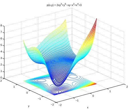
Example 2.6 Consider the following function:

p(x, y) = 2xy2 +y6₋xy₋x2 +x4+ 3

A graph of this function inR3 _{is shown in Figure 2.1. In order to find a lower bound} for the function p(x, y), we can try to maximize γ such that

p(x)−γ is a sum of squares.

γ appears as a new decision variable in the relevant semidefinite programme, which we can optimize over. Indeed, implementation of the sum of squares programme results in the maximum allowable value of γ = 0.9468 achieved at (-1.0799,-0.9752) – infor-mation that may be retrieved from the dual solution of the semidefinite programme.

The above example shows that even if some coefficients of the polynomial are unknown or constrained to lie within certain intervals, checking the sum of squares decomposition can still be done using semidefinite programming. This is helpful, for example when searching for Lyapunov functions for nonlinear systems.

(25)

of the polynomials is high. For this reason, conversion of SOS conditions to the corresponding semidefinite program has been automated in SOSTOOLS, a software developed for this purpose. This software calls SeDuMi [90] or SDPT3 [93], semidef-inite programming solvers, to solve the resulting semidefsemidef-inite program, and converts the solutions back to the solutions of the original SOS programs. These software pack-ages are used for solving all of the examples in this thesis - Example 2.5 is solved, for example, by using the command findsos and Example 2.6 by using the com-mand findbound. A more detailed description of the software can be found in [75]. Moreover, in many examples, the polynomials possess special properties [67] or struc-ture: they are sparse, or bipartite, as we will see in Chapter 4. In this case, we can characterize what monomials are required in Z(x), which reduces significantly the computational burden since the size of the LMIs is reduced, but it also helps improve numerical conditioning. Such structure-exploiting algorithms are available in SOSTOOLS.

2.2

The Positivstellensatz

Real algebraic geometry studies real algebraic sets, i.e., subsets of Rn _{defined by} polynomial equations. There is a fundamental difference between real and complex algebraic geometry, as the field of real numbers is not algebraically closed. Real algebraic geometry deals not only with the zeros of polynomials, but also with domains where the polynomials have a constant sign.

An important result in real algebraic geometry ispositivstellensatz, a theorem that provides an equivalence relation between the emptiness of a semi-algebraic set (i.e., a finite set of polynomial equalities and inequalities), to an algebraic relationship being valid. Along with the algorithmic verifiability of the sum of squares decomposition, they form the pillars of the theory that will be used in the rest of the thesis, unifying and extending known results not only in optimization and control, but also in physics and euclidean geometry [68].

(26)

Definition 2.7 Given polynomials _{h1, . . . , hu} ∈ R[x], the Multiplicative Monoid

generated by the hi is the set of all finite products of hi, including 1. We will denote

this by _M(h1, . . . , hu).

Definition 2.8 Given polynomials{f1, . . . , fs} ∈R[x], the Algebraic Cone generated

by the fj is the set:

C(f1, . . . , fs) =

(

λ0+

X

i

λiFi|Fi ∈ M(f1, . . . , fs), λi ∈Σn

)

. (2.5)

Definition 2.9 Given polynomials _{g1, . . . , gt} ∈R[x], the Ideal generated by the gi

is the set:

I(g1, . . . , gt) =

( X

l

µlgl|µl ∈R[x]

)

. (2.6)

Now can now proceed by quoting Positivstellensatz, a theorem that we will be using frequently in the sequel.

Theorem 2.10 LetR_{be a real closed field. Let}₍_f_j_){_j₌₁_,...,s_},₍_g_l_){_l₌₁_,...,t_}_and₍_h_k_){_k₌₁_,...,u_} be finite families of polynomials inR_[_x₁_{, . . . , x}_n_{]. Denote by}_C _{the Algebraic Cone} gen-erated by (fj){j=1,...,s}, Mthe Multiplicative Monoid generated by (hk){k=1,...,u} and I the ideal generated by (gl){l=1,...,t}. Then the following properties are equivalent:

• The set

{x_∈Rn_|_f_j₍_x₎_≥₀_{, j} _{= 1}_{, . . . , s,} _g_l _{= 0}_{, l} _{= 1}_{, . . . , t,} _h_k₍_x₎₆_{= 0}_{, h}_{= 1}_{, . . . , u}_}

(2.7) is empty.

• There exist f ∈ C, g ∈ I and h∈ M such that:

f +g +h2 = 0. (2.8)

(27)

in convex optimization, where the intersection of two convex sets is empty if and only if there is a hyperplane separating them that certifies the emptiness. Here, the set (2.7) need not be convex, in which case the certificate is not necessarily a hyperplane; the algebraic relationship (2.8) certifies this emptiness.

It should be stressed that there is no guidance as to how, for example, the cone _C should be formed — what the degree or structure of f should be. Putting an upper bound on these degrees and checking whether (2.8) holds, one can create a series of tests for the emptiness of (2.7); each of these tests requires the construction of some sum of squares and polynomial multipliers, resulting in a sum of squares programme that can be solved using SOSTOOLS.

Let us give an example of a problem from combinatorial optimization whose deci-sion verdeci-sion isN P-hard, and for which positivstellensatz results in a series of tests. Example 2.11 Number Partitioning Problem. Consider the optimization ver-sion of Partition:

Problem 2.12 Given a set of n non-negative numbers _{a1, . . . , an}, separate them

into two disjoint sets such that the difference of the subset sums is minimized. The above question can be converted into finding xi =±1, i= 1, . . . , n such that:

F(x) =

n

X

i=1

xiai

is minimized. This is the same problem as

min F2(x) =

n

X

i=1

xiai

!2

s.t. x2_i = 1.

(28)

follows:

max γ

s.t.  



x∈Rn

n

X

i=1

xiai

!2

−γ <0, x2_i = 1, i= 1, . . . , n

 



=∅.

In order to generate the ideal of the polynomials hi(x) , x2i −1 = 0, we look for

polynomials p˜i(x) such that:

I(h1, . . . , hn) =

n

X

i=1

˜

pi(x)hi(x). (2.9)

The cone of f(x),γ−F2₍_x₎ _is

C(f) =σ0(x) +σ1(x)(γ−F2(x)). (2.10)

where σ0(x), σ1(x) are SOS. The monoid of f(x) is f2k where k is a non-negative

integer. Choosing σ0(x) = 0 and k = 1, and structuring the multipliers p˜i(x) =

f(x)pi(x), the overall condition becomes:

max γ

s.t. F2(x)−γ+

n

X

i=1

pi(x)hi(x) is SOS.

While the SOS condition is satisfied and hi(x) = 0 (i.e., xi =±1), F2(x)≥γ, i.e., γ

is a lower bound on the optimal cost.

When thepi(x)are constants, the standard SDP relaxation that was investigated by

(29)

0 2 4 6 8 10 12 0

10 20 30 40 50 60 70 80 90 100 110

W from NPP (rank(W)=1)

n

Success %

p_i(x) constants p_i(x) order 2 p_i(x) order 4

0 2 4 6 8 10 12

0 10 20 30 40 50 60 70 80 90 100 110

W generically full rank

n

Success %

p_i(x) constants p_i(x) order 2 p_i(x) order 4

(a) (b)

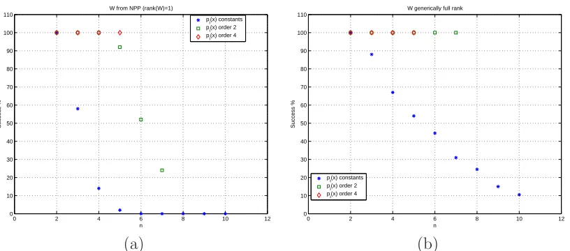
Figure 2.2: Performance of Positivstellensatz tests for the Ising spin glass problem.

In the case of constant pi’s, the problem reduces to

max γ

s.t.



 W −diagp 0

0 −γ+P_ipi



≥0

and using the result by [40] the solution to the above is γ =ha1−Pn_j₌₂aj

i+

, where [_·]+ _{denotes positive projection. When} _n _{is large, then this first positivstellensatz test}

is most likely going to give a trivial lower boundγ, as the probability thata1 ≥Pn_j₌₂aj

is vanishingly small; this is suggested by Figure 2.2(a). Positivstellensatz allows us to write other conditions for nonnegativity, by increasing the order of the polynomials

pi(x). Qualitative results are also shown in Figure 2.2(a) when the pi(x) are allowed

to be of higher degree. In this figure, comparison is made to the true ground states. Alternatively, if W is allowed to be a generically full rank matrix, then better results can be obtained, as shown in Figure 2.2(b). This case has another interpretation: it is related to the problem of finding the ground state of an infinite-range Ising spin glass with couplings Wij drawn from some probability distribution. Such a model is

the Sherrington-Kirkpatrick (SK) [94] spin glass model where the Wij are independent

(30)

Remark 2.13 The special case in which the multiplierspi’s are constants corresponds

exactly to the convex relaxation obtained by standard Lagrangian duality. To make our argument more concrete, consider the general program:

min xTW x

s.t. x2_i −1 = 0

DenoteP =diag(p1, . . . , pn)and Tr(P)the trace of P. The Lagrangian of this problem

is:

L(x, p) = xTW x₋

n

X

i=1

pi(x2i −1) =xT(W −P)x+Tr(P) (2.11)

The dual SDP is therefore:

max Tr(P) s.t. W ₋P _≥0

which gives a lower bound on the optimal value of the primal problem. The ‘dual of the dual’ is easily found to be:

min Tr(W X) s.t. X ≥0

Xii= 1

Now from the original problem, denoting X = xxT _{we see that this can be} _exactly

rewritten as:

xTW x=Tr(W xxT) =Tr(W X) (2.12) where Xii = 1, X ≥0 and X is rank-1. This last, rank-1 condition is what is missing

(31)

A nested family of conditions obtained to test emptiness of sets, under which the more computationally expensive ones are at least as good as the previous ones, can be applied to a tool commonly used in robust control theory, the S-procedure.

Example 2.14 S-procedure. Many times in control theory we must ensure that a certain condition holds whenever some other condition holds. A common test for conditional satisfiability is the S-procedure. We can easily turn the same problem into an emptiness of a set and seek a positivstellensatz test.

In particular, given m symmetric matrices P1, . . . , Pm, consider whether

D:=x∈Rn_:_p_i₍_x_{) =}_xT_P_i_x_≥₀_,_k_x_k_{= 1}_{, i}_{= 1}_{, . . . , m} ₌_∅_.

Using Positivstellensatz, with g(x) = _kx_k2 ₋₁ _and _f₍_x_{) =} P

iσipi(x) +σ0(x), with

σ0(x) an SOS and σi ≥ 0 constants, a sufficient condition for the set D to be empty

is given by the existence of σi that satisfy the condition:

−

m

X

i=1

σixTPix−

n

X

i=1

x2_i is SOS, σi ≥0, (2.13)

which is the standard S-procedure [104]. It is well known that this condition may be conservative, depending on the structure of the set_D. With Positivstellensatz, a hier-archy of polynomial-time computable stronger conditions can be obtained, depending on how the cone _C and ideal _I are constructed. For example, a second test is the following: Assume there exist solutionsσi(x)quadratic polynomials that are SOS and

ρij ≥0 constants to:

−

m

X

i=1

σi(x)pi(x)− m

X

i=1

m

X

j=i+1

ρijpi(x)pj(x)− m

X

i=1

x4_i is SOS. (2.14)

Then, the set D is empty. The search for the σi(x) andρij and the verification of the

(32)

test is always at least as powerful as the standard one, and often strictly stronger.

In the sequel, we will come across various S-procedure type conditions which we test using SOSTOOLS in the framework given above. Instead of using constant multipliers such as the unknownsσiin (2.13), we will be using higher order multipliers

such as the σi(x) in (2.14) – condition that is at least as strong as (2.13) to test the

emptiness of the set _D.

2.3

Conclusion

(33)

Chapter 3

Systems Described by Ordinary

Differential Equations

T yuqrjèretai, jermän yÔqetai,

Ígrän aÎanetai, karfalèon notzetai.

<Hrkleito

Cold things become warm, and what is warm cools; what is wet dries, and the parched is moistened. Heracletus

In this chapter, we will investigate how various analysis questions for nonlinear systems described by Ordinary Differential Equations (ODEs) can be answered using sums of squares (SOS). ODEs have been an important tool for modeling the physical world, ranging from simple mechanical and electrical systems to chemical processes and simplified aircraft dynamics. They have also been the primary tool for modeling components in biological networks or multi-agent systems. Usually, the far-from-equilibrium behavior of such systems is of greater interest than the local ‘linearized’ properties, and most analysis tools for such systems center in what are now known as ‘Lyapunov methods’, named after A. M. Lyapunov. The main feature of these techniques is that system properties are assessed without solving the underlying model equations, but rather through the construction of a function of state (a Lyapunov function) that satisfies certain conditions.

(34)

well as analysis of non-polynomial systems to be performed in a unified manner. The techniques we will be using are based on the sum of squares decomposition and Positivstellensatz, as they were introduced in Chapter 2.

3.1

Introduction

Systems which appear in electrical or mechanical engineering and even biology are usually modeled by a finite number of coupled first-order Ordinary Differential Equa-tions (ODEs) of the form:

˙

x1 = f1(t, x1, . . . , xn),

˙

x2 = f2(t, x1, . . . , xn),

... ...

˙

xn = fn(t, x1, . . . , xn),

where ˙xi denotes the derivative of xi with respect to time, and xi are the state

variables. We use vector notation to describe this system. Let x _∈ Rn _{and let}

f : [0,∞)×Rn_→Rn_{. Then, the above can be written as:}

˙

x=f(t, x). (3.1)

If f(t, x) is piecewise continuous in t and satisfies a local Lipschitz condition in x, then the existence and uniqueness of the solutions is guaranteed locally [35].

In this chapter, we will concentrate on systems that are autonomous, i.e., take the form

˙

x=f(x), (3.2)

(35)

of stability of equilibria which are usually characterized using Lyapunov arguments. Here, we concentrate onstability and asymptotic stability;k · kdenotes a norm inRn_.

Definition 3.1 The equilibrium x= 0 of (3.2) is:

• Stable, if for each ǫ >0 there is δ=δ(ǫ)>0 such that

kx(0)k< δ ⇒ kx(t)k< ǫ, ∀ t ≥0.

• Asymptotically stable if it is stable and δ can be chosen such that

kx(0)k< δ ⇒ lim

t→∞x(t) = 0.

We can see that these definitions of stability involve ǫ−δ formulations, which at first give the impression that a complete description of the flow of the vector field is required to answer stability questions. It is fortunate that in many cases stability can be proved directly by exhibiting an energy-like function, now called a Lyapunov function[35, 107]. This is Lyapunov’s direct method. Under some technical conditions, the existence of this function was also proved necessary for asymptotic stability [27]. More precisely, the conditions are stated in the following theorem: Theorem 3.2 ([35]) Consider the system (3.2), and let D_⊆ Rn _{be a neighborhood} of the origin. If there is a continuously differentiable function V :D → R _{such that} the following two conditions are satisfied:

(36)

In the case of linear time-invariant systems

˙

x=Ax, (3.3)

the stability properties can be characterized by the locations of the eigenvalues λi of

the matrix A, or equivalently, through a Lyapunov argument as follows:

Theorem 3.3 [35] The matrix A is a stability matrix; that is Reλi < 0 for all

eigenvaluesλi of A if and only if for any given positive definite matrix Q there exists

a positive definite matrix P that satisfies:

P A+ATP =−Q. (3.4)

P is unique, and V =xT_{P x} _{is a Lyapunov function for (3.3).}

We see that the construction of the Lyapunov function in the case of linear sys-tems is reduced to solving an appropriate Algebraic Lyapunov Equation (3.4). Al-ternatively, P can be obtained by solving two Linear Matrix Inequality (LMI) [10] conditions:

P > 0,

ATP +P A < 0.

A feasible P exists if and only if A is Hurwitz. LMIs are constraints in semidefinite programs [96], which can be solved using algorithms with a worst-case polynomial time complexity. This makes them particularly attractive for computation.

(37)

sys-tem has imaginary axis eigenvalues and the result is valid anyway only locally. Other methodologies involve absolute stability theory [19], Linear Parameter Varying (LPV) embeddings [23, 86, 53], Integral Quadratic Constraint (IQC) formulations [47] and others.

In this chapter, we will build on the methodology introduced in [66] and we will show how to use the sum of squares decomposition to analyze different classes of systems described by ODEs using Lyapunov methodologies. There are mainly two reasons why there has been no algorithmic methodology for constructing the Lya-punov functions V(x) for so long. On one hand, the ‘terms’ that should appear in

V(x) are not knowna priori, and on the other hand, testing the nonnegativity condi-tions in Theorem 3.2 is a difficult task even in the case in which they are polynomial. We can get to the bottom of the first problem by resorting to intuition and prior knowledge of energy-like terms that are likely to appear in V(x). As far as the sec-ond problem is concerned, this is closely related to the fact that testing polynomial nonnegativity when the degree is greater than or equal to 4 is an _{N P}-hard problem, as was mentioned in the previous chapter [50].

For concreteness, let us assume that f(x) is a polynomial vector field. Suppose that we also wish to construct a V(x) that is also polynomial in x. In this case, the two conditions in Theorem 3.2 become polynomial nonnegativity conditions. To circumvent the difficult task of testing them, we can restrict our attention to cases in which the two conditions admit SOS decompositions. Note that even if the coefficients of a polynomial Lyapunov candidateV are unknown, we can still search for them so that the two Lyapunov conditions are satisfied, as was explained in the previous chapter.

To impose thatV(x) should be positivedefinite rather than positive semi-definite, we construct an auxiliary positive definite ‘shaping’ function ϕ(x) as follows:

ϕ(x) =

n

X

i=1

d

X

j=1

ǫijx2ij, m

X

j=1

ǫij ≥γ ∀ i= 1, . . . , n, γ >0, ǫij ≥0 ∀ i, j (3.5)

(38)

obviously

V(x)−ϕ(x)≥0⇒V(x)≥ϕ(x)>0. (3.6) Therefore, we have

Proposition 3.4 Given a polynomial V(x) of degree 2d, let ϕ(x) be given by Equa-tion (3.5). Then, the condiEqua-tion

V(x)₋ϕ(x) is a sum of squares (3.7)

guarantees the positive definiteness of V(x).

In the case of global stability, i.e., for D=Rn_{, the conditions in Theorem 3.2 can} then be formulated directly as SOS conditions. Therefore, we have the following sum of squares program:

Program 3.5 To construct a Lyapunov function for system (3.2),

Find a polynomial V(x), V(0) = 0

and a positive definite function ϕ(x) of the form (3.5) such that

V(x)−ϕ(x) is SOS (3.8)

− ∂V_∂xf(x) is SOS (3.9)

Then V(x) is a Lyapunov function for system (3.2) and the zero equilibrium of (3.2) is globally stable.

(39)

globally [35]. Also, if condition (3.9) is replaced by

−∂V

∂xf(x)−ψ(x) is SOS, (3.10)

where ψ(x) is a positive definite polynomial constructed as per (3.5), then ˙V(x) is negative definite and the origin is globally asymptotically stable.

Below is an example of how the construction of a Lyapunov function is performed using SOSTOOLS.

Example 3.6 Consider the system

˙

x1 = −x1+x32−3x3x4

˙

x2 = −x1−x32

˙

x3 = x1x4−x3

˙

x4 = x1x3−x34,

which has the only equilibrium at the origin. As a first attempt, we will try to construct a quadratic Lyapunov function of the form V =P4_i₌₁P4_j₌_iaijxixj where theaij’s are

the unknowns. We search for V that satisfy the conditions in Program 3.5.

It turns out that a Lyapunov function of the above form does not exist (the cor-responding semidefinite program is infeasible), so we will next search for a quartic Lyapunov function. One then finds a Lyapunov function that satisfies conditions (3.8) and (3.10), and thus proves global asymptotic stability of the origin. To three significant figures, this reads:

V = 1.12x1x2x32−0.785x1x2+ 0.713x32x1+ 0.500x1x2x24+ 0.768x44

+1.64x21+ 1.76x23 + 0.392x22+ 1.63x24+ 1.69x12x22+ 0.557x43

+0.724x31x2 + 0.181x41+ 1.07x24+ 0.561x21x32+ 1.61x22x23

+0.525x2

1x24 + 0.969x22x24+ 0.569x23x42−0.251x4x3x1+ 0.432x4x3x2.

(40)

3.2

Stability of Constrained Systems

In this section, we extend Lyapunov’s theorem to systems that evolve under equality, inequality, and integral constraints. This is a very general class of systems, special cases of which are differential algebraic equations, robust stability analysis and per-formance formulations. It will also allow us to treat non-polynomial vector fields exactly.

Inequality constraints arise naturally when considering positive systems: systems with inherently positive states, e.g., a chemical reaction in which the concentrations of the reactants are positive. The same type of constraints can be used to describe uncertain parameter sets for the study of robust stability of systems in the presence of parametric uncertainty.

On the other hand, systems evolving over a manifold described by a set of equal-ity constraints arise in a plethora of cases, and are also called differential algebraic equations or descriptor systems [16]. Examples of equality constraints are holonomic (configuration) constraints in mechanical systems and conservation laws – in electrical networks in the form of current balance and in chemical engineering in the form of mass balance. Sometimes it is possible to back-substitute and reduce the system to an ordinary differential equation, but this usually results in more complicated vector fields of higher order. In some other cases, this is not possible and a differential index theory was developed as a measure of this singularity [91]. Equality constraints also prove useful in robust stability analysis where they appear as constraints guaranteeing that the equilibrium of the system is at the origin.

The last type of constraints that are going to be incorporated is of integral type, in particular Integral Quadratic Constraints (IQCs) [47]. They provide a framework rich enough to encapsulate many types of uncertainty and unmodelled dynamics: dynamic, time-varying and L2 bounded uncertainty, just to name a few. Moreover,

one can formulate performance calculations using IQCs such as_L2 input-output gain

(41)

Consider the nonlinear system

˙

x = f(x, u), (3.11)

with the following inequality, equality, and integral constraints that are satisfied by

x and u:

ai1(x, u)≤0, for i1 = 1, ..., N1, (3.12)

bi2(x, u) = 0, for i2 = 1, ..., N2, (3.13)

RT

0 ci3(x, u)dt≤0,for i3 = 1, ..., N3, and ∀ T ≥0. (3.14)

Herex_∈Rn_{is the state of the system, and}_u_∈Rm_{is a collection of auxiliary variables} (such as inputs, non-polynomial functions of states, uncertain parameters, etc). We assume that f(x, u), apart from the required Lipschitz conditions for existence of solutions, has no singularity inD, whereD ⊂Rn+m _{is defined as}

D =_{(x, u)_∈Rn+m_|_a_i

1(x, u)≤0, bi2(x, u) = 0, for all i1 and i2}.

Without loss of generality, it is also assumed that f(x, u) = 0 forx= 0 and u∈ D0

u,

where

D0

u ={u∈Rm|(0, u)∈ D}.

The following theorem is an extension of Lyapunov’s stability theorem, and can be used to prove that the origin is a stable equilibrium of the above system. It uses a technique reminiscent of the well-known S-procedure [104] in nonlinear and robust control theory, that was discussed in Example 2.14.

(42)

0, p2i₁(x, u)≥0, q1i₂(x, u), q2i₂(x, u) and constants ri3 ≥0 such that

V(x) +Xp1i₁(x, u)ai1(x, u) +

X

q1i₂(x, u)bi2(x, u)>0, (3.15)

− ∂V_∂xf(x, u) +Xp2i₁(x, u)ai1(x, u) +

X

q2i₂(x, u)bi2(x, u) +

X

ri3ci3(x, u)≥0

(3.16)

Then the origin of the state space is a stable equilibrium of the system. Proof. If condition (3.15) is fulfilled, then we have that in D

V(x)>₋Xp1i₁(x, u)ai1(x, u)−

X

q1i₂(x, u)bi2(x, u)≥0,

and so V(x)>0 in _D, whereai1(x, u) and bi2(x, u) satisfy (3.12).

Condition (3.16) can be integrated from time t= 0 to t=T to obtain

V(0)₋V(T)_{≥ −}X

Z T

0 {

p2i₁(x, u)ai1(x, u)−ri3ci3(x, u)}dt≥0,

where we have used the fact thatai1(x, u),bi2(x, u) andci3(x, u) satisfy (3.12)–(3.14).

This shows that the Lyapunov function is non-increasing along the trajectories of the system, and is positive definite in D. Therefore, the conditions for Lyapunov stability (see Theorem 3.2) are satisfied. The rest of the proof is similar to the proof of Lyapunov’s theorem, which can be found in many standard textbooks, e.g., [35].

We note that even though the integral constraints used above are required to hold for all T _≥ 0 (i.e., hard integral constraints), most of the ones that one can develop during an analysis method are soft, i.e. they need not hold for finite-time intervals. In the case of soft Integral Quadratic Constraints, non-causal multipliers were used for stability analysis. See [47] for more details.

(43)

of systems with constraints. The procedure is similar to the one for the case of unconstrained systems described in the previous section, and is based on relaxing the conditions in Theorem 3.7 to SOS conditions. For this, we need to make some assumptions, some of which will be removed in the sequel.

• The vector field fx(x, u) is assumed to be polynomial or rational, and the

con-straint functionsai1(x, u),bi2(x, u),ci3(x, u) are assumed to be polynomial. This

assumption will be removed in a later section through a recasting process.

• We search for bounded degreepolynomial Lyapunov functionV and multipliers

pi1, qi1, i1 = 1, . . . , N1 and pi2,qi2, i2 = 1, . . . , N2.

To make the above concrete, in order to use Theorem 3.7 and the sum of squares decomposition, we have the proposition below.

Proposition 3.8 Suppose that for system (3.1) with f(x, u) = n_d₍(_x,ux,u)₎ where n(x, u) and d(x, u) are polynomials and d(x, u) > 0 in _D, there exist polynomial functions

V(x), p1i₁(x, u), p2i₁(x, u), q1i₂(x, u), q2i₂(x, u), a positive definite function ϕ(x) of

the form given in Equation 3.5 and constants ri3 ≥0 such that

V(x) +Xp1i₁(x, u)ai1(x, u) +

X

q1i₂(x, u)bi2(x, u)−ϕ(x) is SOS, (3.17) p1i₁(x, u), p2i₁(x, u) are SOS for i1 = 1, . . . , N1, (3.18)

d(x, u)



 −

∂V

∂xf(x, u) +

P

p2i₁(x, u)ai1(x, u)

+Pq2i₂(x, u)bi2(x, u) +

P

ri3ci3(x, u)



 is SOS. (3.19)

Then the origin of the state space is a stable equilibrium of the system.

The polynomials V(x), p1i₁(x, u), p2i₁(x, u), q1i₂(x, u),q2i₂(x, u), the constants ri3

and the positive definite function ϕ(x) can be constructed using SOSTOOLS [75], and a program similar to Program 3.5 can be constructed.

(44)

3.3

Estimating the Region of Attraction

In many instances, non-global stability analysis may be the objective, i.e., when dealing with physical models with positivity constraints on the states (often referred to as positive systems [42]), or when several equilibria or limit cycles are present. In such cases, one may define regions of interest using inequality constraints.

For example, let us consider local stability analysis of the zero equilibrium of ˙

x=f(x). Define the following inequality constraint on x:

a(x),xTx₋ξ _≤0, (3.20)

where ξ is a positive constant. Then local stability of the zero equilibrium can be tested using the next corollary.

Corollary 3.9 Suppose for the system x˙ =f(x)and the inequality constrainta(x)≤

0given in (3.20) there exist a polynomial functionV(x)and SOS polynomialsp1(x), p2(x)

such that

V(x) +p1(x)a(x)−ϕ(x) is SOS,

− ∂V

∂xf(x) +p2(x)a(x) is SOS,

where ϕ(x) is as defined in Equation (3.5). Then the zero equilibrium of the system is stable.

A problem of particular interest is estimation of the region of attraction of an equilibrium. An estimate of the region of attraction is the largest level set of V(x) obtained from the previous corollary which can ‘fit’ in the region described bya(x)≤

0. More specifically, given a Lyapunov function V(x) and a domain D in which a Lyapunov function satisfying the conditions of asymptotic stability was constructed, we seek aγ >0 such that Ωγ ={x∈Rn|V(x)≤γ}is bounded and strictly contained

inD; then Ωγ is an estimate of the region of attraction. In order to get the maximum

(45)

follows:

{x∈Rn _:_V₍_x₎_{< γ, a}₍_x_{) = 0}_}₌_∅ _(3.21)

Positivstellensatz conditions take the form:

N

X

i=1

x2_i

!r

(V(x)₋γ) +p(x)a(x) is a SOS (3.22)

where r is a non-negative integer and p(x) is a polynomial. Therefore, the task of finding the maximum γ can be formulated as the following sum of squares program: Program 3.10 Program to find the maximum γ such that _{x _∈ Rn_|_V₍_x₎ _{< γ}_{} ⊂}

{x_∈Rn_|_a₍_x₎_≤₀_}_:

Given V(x), a(x), maximize γ and find a non-negative integer r

and a polynomial p(x) such that

N

X

i=1

x2_i

!r

(V(x)₋γ) +p(x)a(x) is a SOS.

In order to find good estimates of the region of attraction, one has to iterate between V(x) and a(x).

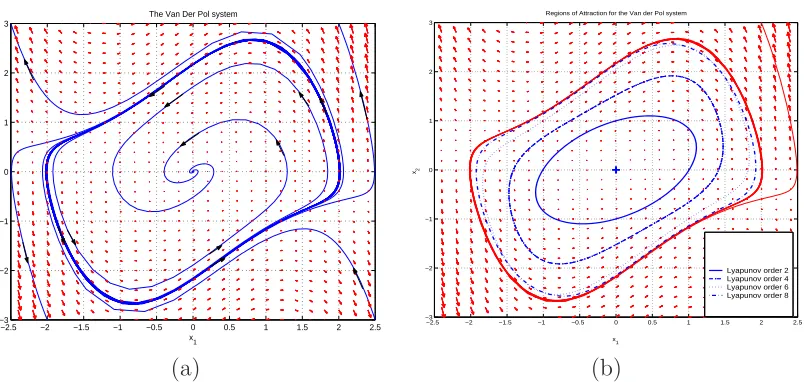
Example 3.11 Consider the Van der Pol equation in reverse time:

˙

x1 = −x2 (3.23)

˙

x2 = x1−(1−x21)x2 (3.24)

The phase plane is shown in Figure 3.1(a); the presence of an unstable limit cy-cle makes the stability of the only equilibrium local. In this case, we are interested in determining how far from the origin we can choose an initial condition and the trajectory will still converge to the origin. To obtain an estimate of the region of attraction of the zero equilibrium of (3.23–3.24), we first initialize a(x) = xT_x₋_ξ_,

(46)

−2.5 −2 −1.5 −1 −0.5 0 0.5 1 1.5 2 2.5 −3

−2 −1 0 1 2 3

x₁

x2

The Van Der Pol system

−2.5 −2 −1.5 −1 −0.5 0 0.5 1 1.5 2 2.5

−3 −2 −1 0 1 2 3

x1 x2

Regions of Attraction for the Van der Pol system

Lyapunov order 2 Lyapunov order 4 Lyapunov order 6 Lyapunov order 8

(a) (b)

Figure 3.1: The Van der Pol system in reverse time, with estimates of the region of attraction of the stable equilibrium.

find the maximum γ such that V(x)₋γ is completely contained in the set V˙(x)_≤0. We then set a(x) = V(x)−γ, and increase the order of V(x) by 2. We can then find a new Lyapunov function of this order adjusting γ, iterating between V(x) and

a(x). Estimates of the region of attraction in the formV(x)≤γ were constructed for different degree V(x), shown in Figure 3.1(b).

3.4

Analysis of Systems with Non-Polynomial

Vec-tor Fields

Thus far, we have concentrated on systems that are described by polynomial vector fields. It is true that physical systems, the functionality of which is in the focus of many research areas, seldom are modeled by polynomial vector fields.

In this section, we will build on a recasting process [82] that produces a polynomial system description from a non-polynomial one, with state dimension at least the same as the original system or higher. The stability properties of the original system can be concluded from the analysis of the recasted system [63]. To describe the original system faithfully, constraints of the form xn+1 =F(x1, ..., xn) that are created when

(47)

ann-dimensional manifold on which the solutions to the original differential equations lie. In general such constraints cannot be converted into polynomial forms, even though sometimes there exist polynomial constraints that are induced by the recasting process. For example:

• Two variables introduced for trigonometric functions such as x2 = sinx1, x3 =

cosx1 are constrained via x22+x23 = 1.

• Introducing a variable to replace a power function such as x2 = √x1 induces

the constraints x2

2−x1 = 0, x2 ≥0.

• Introducing a variable to replace an exponential function such as x2 = exp(x1)

induces the constraint x2 ≥0.

We will identify two different classes of systems. We consider systems with non-polynomial vector fields that under a change of variables are transformed into poly-nomial with:

1. Only polynomial equality constraints; 2. Non-polynomial equality constraints.

A particular example of case (1) above is the simple pendulum, which is described by:

d dt



 θ

ω 

=



 ω

−gl sinθ





where g is the gravitational constant, l is the length of the pendulum, ω its angular velocity andθ the angular deviation of the bead from the vertical. Settingx1 = sinθ

and x2 = cosθ, one can easily rewrite the above system as

d dt



   

x1

ω

x2



   

=



   

x2ω

−glx1

−x1ω



   

(48)

where the constraintx2

1+x22 = 1 is a polynomial equality in (x1, x2) that restricts the

3-D recasted system to the original 2-D system.

However, in some cases (case (2) above), this technique results in a series of equality constraints that are not polynomial equalities, for example, relating sin(θ) and θ. These appear many times because of modeling descriptions. For example, in order to model enzymatic reactions in biological systems [48], it is common practice to use vector fields with non-rational powers, in the Michaelis-Menten sense. Also, the model of an aircraft in longitudinal flight contains trigonometric nonlinearities of the angle of attack and pitch angle, but in the same equations, one usually captures the coefficients of lift and drag as polynomial descriptions of these variables. The stability analysis of the closed loop system using the above methodology becomes difficult, as the same variable appears both in polynomial and non-polynomial terms. The same is true in the case of analysis of chemical processes, where the temperature appears in the energy equation both as a state and also exponentiated in Arrhenius law for the reaction rate.

Suppose that for a nonpolynomial system

˙

z =f(z) (3.25)

which has an equilibrium at the origin, the recasted system obtained using a recasting procedure is written as

˙˜

x1 =f1(˜x1,x˜2), (3.26)

˙˜

x2 =f2(˜x1,x˜2), (3.27)

where ˜x1 = (x1, ..., xn) = z are the state variables of the original system, ˜x2 =

(xn+1, ..., xn+m) are the new variables introduced in the recasting process, andf1(˜x1,x˜2),

f2(˜x1,x˜2) are polynomial in their arguments.

(49)

polynomial ones) by

˜

x2 =F(˜x1), (3.28)

and those that arise indirectly (the non-polynomial ones) by

G1(˜x1,x˜2) = 0, (3.29)

G2(˜x1,x˜2)≤0, (3.30)

whereF,G1, andG2are column vectors of functions with appropriate dimensions, and

the equalities or inequalities hold entry-wise. We should keep in mind that constraints (3.29)–(3.30) are satisfied only when ˜x2 =F(˜x1) are substituted to (3.29)–(3.30). We

assume that all functions involved are polynomials in their arguments.

Proving stability of the zero equilibrium of the original system (3.25) amounts to proving that all trajectories starting close enough to z = 0 will remain close to this equilibrium point. This can be accomplished by finding a Lyapunov function V(z) that satisfies the conditions of Lyapunov’s stability theorem. Here we use the recasted system to construct a Lyapunov function that proves stability of the equilibrium of the original system. Sufficient conditions that guarantee the existence of a Lyapunov function are stated in the following proposition.

Proposition 3.12 Let _D1 ⊂ Rn and D2 ⊂ Rm be open sets such that 0 ∈ D1

and F(D1) ⊆ D2. Furthermore, define x˜2,0 = F(0). If there exists a function

˜

(50)

and σ2(˜x1,x˜2) with appropriate dimensions such that

˜

V(0,x˜2,0) = 0, (3.31)

˜

V +λT₁G1 +σ1TG2−φ(˜x1,x˜2)≥0 ∀(˜x1,x˜2)∈ D1× D2, (3.32)

− ∂V˜

∂x˜1

f1−

∂V˜ ∂x˜2

f2+λT2G1 +σ2TG2 ≥0 ∀(˜x1,x˜2)∈ D1× D2, (3.33)

σ1(˜x1,x˜2)≥0 ∀(˜x1,x˜2)∈Rn+m, (3.34)

σ2(˜x1,x˜2)≥0 ∀(˜x1,x˜2)∈Rn+m, (3.35)

for some scalar function φ(˜x1,x˜2) with φ(˜x1, F(˜x1))>0 ∀x˜1 ∈ D1\ {0}, then z = 0

is a stable equilibrium of (3.25).

Proof. Define V(z) = ˜V(z, F(z)). From (3.31) and (3.32), it is straightforward to verify that the first Lyapunov condition is satisfied by V(z). In fact, from (3.29)– (3.30), (3.32) and (3.34), we have that

V(˜x1,x˜2)≥φ(˜x1,x˜2)−λT1G1−σT1G2 ≥φ(˜x1,x˜2) ∀(˜x1,x˜2)∈ D1× D2.

Sinceφ(z, F(z))>0 ∀z ∈ D1\{0}andF(D1)⊆ D2, it follows thatV(z)>0 ∀z ∈

D1\ {0}.

Finally, by the chain rule of differentiation we have

∂V

∂z (z)f(z) =

∂V˜ ∂x˜1

(z, F(z))f1(z, F(z)) +

∂V˜ ∂x˜2

(z, F(z))f2(z, F(z)),

and using the same argument as above in conjunction with (3.29)–(3.30), (3.33) and (3.35), we see that the second Lyapunov condition is satisfied. Therefore, V(z) is a Lyapunov function for (3.25) and z = 0 is a stable equilibrium of the system.

(51)

as a semialgebraic set:

D1× D2 ={(˜x1,x˜2)∈Rn×Rm :GD(˜x1,x˜2)≥0},

where GD(˜x1,x˜2) is a column vector of polynomials and the inequality is satisfied

entry-wise.

Let us now give an example of how this methodology can be used.

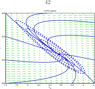
Example 3.13 (Continuously Stirred Tank Reactor) Chemical reactors are the most important unit in a chemical process. Here, we consider the analysis of the dynamics of a perfectly mixed, diabatic, continuously stirred tank reactor (CSTR) [3]. We also assume a constant volume – constant parameter system for simplicity.

The reaction taking place in the CSTR is a first-order exothermic irreversible reaction A _→ B. After balancing mass and energy, the reactor temperature T and the concentration of species A in the reactor CA evolve as follows:

˙

CA =

F

V (CAf −CA)−k0e

−∆E

RTC

A (3.36)

˙

T = F

V (Tf −T)−

∆H

ρcp

k0e−

∆E

RTC

A−

U A

V ρcp

(T ₋Tj) (3.37)

where F is the volumetric flow rate,V is the reactor volume, CAf is the concentration

of A in the freestream, k0 is the pre-exponential factor of Arrhenius law, ∆E is the

reaction activation energy, R is the ideal gas constant, Tf is the feed temperature,

−∆H is the heat of reaction (exothermic), ρ is the density, cp is the heat capacity, U

is the overall heat transfer coefficient, A is the area for heat exchange, and Tj is the

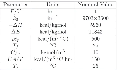
jacket temperature. For the analysis, we use the values shown in Table 3.1.

The equilibrium of the above system is given by (CA0, T0) = (8.5636,311.171). We

employ the following transformation: x1 = CA/CA0 −1, x2 = T /T0 −1; this serves

(52)

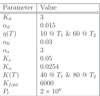
Parameter Units Nominal Value

F/V hr−1 ₁

k0 hr−1 9703×3600

−∆H kcal/kgmol 5960 ∆E kcal/kgmol 11843

ρcp kcal/(m3◦C) 500

Tf ◦C 25

CAf kgmol/m

3 ₁₀

U A/V kcal/(m3◦C hr) 150

Tj ◦C 25

Table 3.1: Parameter values for the Continuously Stirred Tank Reactor (CSTR) system.

state to reduce numerical ill-conditioning. The transformed system then becomes:

˙

x1 =

F V

_C

Af

CA0

−(x1+ 1)

−k0e−

∆E

RT₀₍x₂₊₁₎₍_x

1+ 1)

˙

x2 =

F V

Tf

T0 −

(x2+ 1)

− ∆HCA0

ρcpT0

k0e−

∆E

RT₀₍x₂₊₁₎₍_x

1+ 1)−

U A

V ρcp

(x2+ 1)−

Tj

T0

Note that the system has an exponential term; the recasting will yield an indirect constraint, as discussed earlier in this section. Define the state x3 = e

∆Ex₂

RT₀₍x₂₊₁₎ −_1.

Then an extra equation in the analysis would be

˙

x3 =

∆E

RT0(x2+ 1)2

(x3+ 1) ˙x2

under the constraint that x3 >−1.

Then the full system, after we use the equilibrium relationship simplifies to:

˙

x1 = −

F

V x1−k0e

−∆E

RT₀(x

1x3+x1+x3) (3.38)

˙

x2 = −

F

V x2−

∆HCA0

ρcpT0

k0e−

∆E

RT₀₍_x

1x3+x1+x3)−

U A

V ρcp

x2 (3.39)

˙

x3 =

∆E

RT0(x2+ 1)2

(x3+ 1) ˙x2 (3.40)

(53)

7.6 7.8 8 8.2 8.4 8.6 8.8 9 9.2 305

310 315 320

C_A

T

CSTR system

Figure 3.2: Lyapunov function level curves for the Continuously Stirred Tank Reactor system.

proceed, we define the set _D1 as:

D1 ={(x1, x2)∈R2 :|x1| ≤γ1,|x2| ≤γ2}

and then define the set D2 as

D2 ={x3 ∈R: (x3−e

−∆Eγ₂

RT₀₍−γ₂₊₁₎ −1)(x

3 −e

∆Eγ₂

RT₀₍γ₂₊₁₎ −1)≤0}

Then the system is ready for analysis as per Proposition 3.12. For γ1 = 0.12 and

γ2 = 0.05, a quartic Lyapunov function can be constructed for the system described

by Equations (3.38)–(3.40) using Proposition 3.12. Here the following φ(x) is used:

φ(x) =

2

X

i=1

X

j=2,4

ǫi,jxji +

4

X

j=1

ǫ3,jxj3,

with

ǫ1,2+ǫ1,4−0.1≥0

ǫ2,2+

Scalable analysis of nonlinear systems using convex optimization

Using Convex Optimization

Abstract

Contents

List of Figures

List of Tables

Outline and Contributions

FDEs/ PDEs

System size

Large-Scale ODE Internet Network

Chapter 2

Nonnegativity and the Sum of Squares

The Positivstellensatz

Conclusion

Introduction

P A+ATP =−Q. (3.4)

Stability of Constrained Systems

Estimating the Region of Attraction

Analysis of Systems with Non-Polynomial