DOI: http://dx.doi.org/10.26483/ijarcs.v8i8.4706
Volume 8, No. 8, September-October 2017
International Journal of Advanced Research in Computer Science
RESEARCH PAPER
Available Online at www.ijarcs.info
ISSN No. 0976-5697
FUZZY NON-LINEAR OPTIMIZATION MODEL FOR PRODUCTION LINE
BALANCING OF JADHAV INDUSTRIES USING GENETIC ALGORITHM
Mr. Girish R. Naik
Associate Professor, Production Department KIT’s College of Engineering
Kolhapur, India
Dr. V.A.Raikar
Director,
SSDGCT’S Sanjay Ghodawat Group of Institutions Atigre, Kolhapur, India.
Dr. P.G. Naik
Professor
Department of Computer Studies ChatrapatiShahu Institute of Business
Education and Research Kolhapur, India
Abstract: In a manufacturing industry production line balancing poses a significant challenge owing to the trade-off between machine idle time and Work-In-Process accumulation between different machines. Several models have been proposed to solve the problem thereby improving the line efficiency. The lowest common denominator in all such approaches is to attain an optimal level of service keeping the total cost associated with service cost and the waiting cost at its minimum. Most of the models proposed till date employ hard computing techniques which poses high mathematical complexity as the number of machines in the line increase. Hard computing techniques are tolerable to moderate sized production lines and break when the size of the line increases beyond the limits. To address this issue, several soft computing techniques have been devised in literature which are logical in nature in contrast to the mathematical nature of hard computing counter parts. Further, soft computing techniques have the power of reducing NP-Hard problems to be solvable in polynomial time. In the current paper, the authors have applied nonlinear fuzzy-GA optimization model for solving production line balancing problem of Jadhav Industries Pvt. Ltd, Kolhapur. The results obtained are compared with their crisp counterparts.
Keywords : Cross-Over, Defuzzification, Fuzzy Ranking, PLBP, Membership Function, Mutation, Non-linear Optimization, WIP
1. INTRODUCTION
The production line balancing problems are basically used to suggest ways and means for improving the line efficiency. The common approach is to analyze and reach an optimal service level keeping in mind the cost associated such as service cost and waiting cost.
The planning and design of sequential work activities into different work stations in order to gain high utilization of input resources, thereby achieving minimization of idle time is referred to as “Production Line Balancing Problem” (PLBP).
In their research work, the authors have focused on several aspects of production line balancing problem with an objective:
• To achieve the optimal balance of cost by determining the service level minimizing total expected system service cost and the total expected system waiting cost by considering imprecision or vagueness in input parameters and to compare the outcomes of the crisp expert system model with the corresponding fuzzy expert system model.
• To analyze production line for bottleneck resources and to redesign the production line to overcome the limitations offered by constrained resources.
• To study system utilization and cost incurred for cycle time management and minimizing non-value added
component of cycle time for determining line performance at various levels of service and determine line efficiency. To achieve feasible optimal level through waste minimization In flow type of manufacturing system in the production line, whenever the arrival rate of items exceeds the serving capacity of work station, the items arriving cannot receive immediate service due to busy work stations, which results in accumulation of excess WIP (Work In Process) between work stations. The objective of current research is to design a generic multi-channel, multi-phase production line for
Optimizing total cost consisting of cost of service and cost of waiting
Analyzing bottleneck resources
Cycle time management by minimization of non-value added component
Determining optimal level of service
Determining line performance at various level of services Determining line efficiency and to provide organization with up to date information on system status at any point of time.
2. LITERATURE REVIEW
Minimization of smoothness index and cost of equipment and cycle time minimization are the major objectives focused by the researchers. Most of the work deals with multi objective decision method based on min-max and weighted approach proposed to solve specific problems. A small size nine task problem was solved to present the systematic procedure for obtaining pareto optimal solution. Determination of Work In Process level for achieving the shorter cycle time for meeting desired throughput requirements was focused [1]. The authors have proposed a WIP determination model that takes into account bottleneck workstation and time constraints into account [2]. Three different algorithms based on tabu search for the problems ranging from small, medium to large size are proposed. The issues related to variable performance of work stations, changing operational requirements and causes of frequent bottlenecks are considered [3]. This helps organizations to design their production line as per the objectives of organization. A study on integration of parameters for line balancing application is carried out. Authors have analyzed communication between the Work Place Planners (WPP) and line balancing applications with AutoCAD based on integrated simulation [4, 5]. Process time in a continuous production line is considered [6]. The main issues are queuing among work stations. The focus is on minimization of queuing problem. The approach employed is multi objective model and genetic algorithm procedure for obtaining best solution. 25% decrease in queue time and 30% decrease in cost is reported by the authors in their study on production line in automobile manufacturing. A sequential approach for balancing an assembly line with a focus on dual objectives of balancing loss and system loss minimization is presented [7]. The approach presented is generic and is capable of solving different line assembly problems within a reasonable computation time. A numerical example has been added to demonstrate the generic nature of the approach. The technical constraint focusing on the minimization of a queuing problem and regulation of the workers by applying hybrid models was carried out. The outcome of the Mixed Models (MM) assists in the reduction of the queuing time and the idling time through the harmonization of the tasks in each workstation [8]. A study on the effectiveness of three manufacturing rules viz., line balancing, on-time delivery, and utilization of bottleneck resources was carried out [9]. Performance matrix for these parameters is considered and guide line based on different factory conditions is provided. A classification scheme for balancing of assembly line is provided [10]. This is a significant step towards identification of the remaining research challenges which might contribute to bridge the gap. The production control problems arising in two-station serial production systems subject to Process Queue Time (PQT) constraints was examined [11] and was solved by efficient algorithm to significantly reduce computational complexity. An innovative method based on Particle Swarm Optimization (PSO) for the simple assembly line balancing problem (SALBP), a well-known NP-hard manufacturing problem is presented [12].Optimization based on dual objectives of production rate and work load smoothing maximization of the line is considered. Survey of the developments in general assembly line research is carried out [13, 14]. Besides enlisting recent trends, solutions to real world
problems are presented. Goal programming model is proposed for U line to meet flexibility requirements of line [15]. A mathematical model and innovative procedures for the single model assembly line balancing problem with parallel lines is proposed [16]. The significance of procedures is presented with suitable numerical examples. The production line of Bangladesh Machine Tool Factory line was analyzed by the authors which was previously incurring loss for a long time. The line was considered to minimize no. of workstations and cycle time. The line was redesigned and efficient heuristic approach was applied to line which resulted in a significant improvement [17]. Application of an efficient heuristic approach has been illustrated for solution of the deterministic and single-model Assembly Line Balancing problem. The main objective of the work was to improve the efficiency of the line by minimizing the number of workstations with minimum cycle time. The production line was redesigned by employing Longest Operation Time (LOT) method based on heuristic approach [18]. In order to balance parallel assembly lines a novel approach based on multiple-colony ant algorithm was proposed [19]. The algorithm proposed was one of the first initiatives in modeling and solving similar problems with swarm intelligence based technique. A Bi level Differential Evolution algorithm to solve a Flexible Assembly Line scheduling problem is presented [20].A model based on scatter search algorithm and a mixed integer linear programming was proposed for solving multistage scheduling problem in a batch production environment. Review of problems pertaining to scheduling and process planning in a flow shop and job shop manufacturing environment has been carried out to understand computational approaches for manufacturing optimizations [21, 22].
3. CONCEPTUAL MODEL
In a production line consisting of n machines, M1, M2,. . . ,
Mn, due to the varying cycle times of the machines, the time
at which the product enters nth machine is given by [23],
Max [ Max [ Max [ . . . [ Max [ ], , . . . . ], ]
(1)
The authors consider the two cases given by:
Case 1 : CTM1 < CTM2 < CTM3 < . . . < CTMi
In this case each machine is continuously busy processing the products. Hence the idle time of any machine is zero. However, it results in WIP accumulation between machines. In this case, in equn (1), second term will be maximum as shown below and hence selected in the expression.
CTM1 < CTM2
Adding to CTM1 both the sides, we get
2CTM1 < CTM1 + CTM2
2CTM1 <
Hence, Max =
= Max =
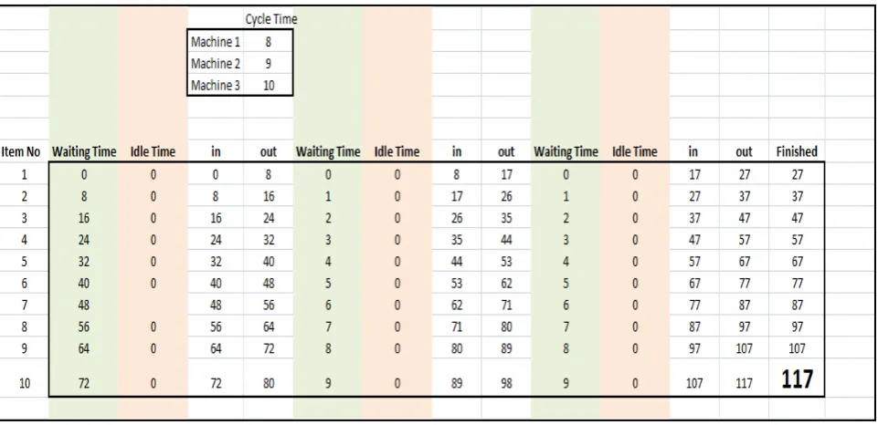
Consider the production line containing three machines M1,
M2, M3 with the corresponding cycle times given by 8 min,
9 min and 10 min, respectively. In this case, CTM1 <CTM2 <CTM3
The total time required for processing of N products in this case is given by
Hence, time required for processing of 10 products is given by,
27 + 72 + 9 (1) + 9 (1) = 117 min
The same is illustrated by implementing the model in MS-Excel as shown in Figure 1(a).
Figure 1(a). First Hand Implementation of Conceptual Model in MS-Excel
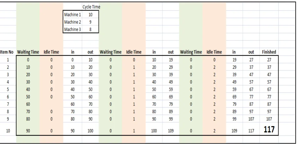
Case 2 : CTM1 >CTM2 >CTM3
In this case each machine, except the first one is idle waiting for the product. Hence the WIP accumulation is zero. In this case in equn(1), first term will be maximum as shown below: We have, CTM1 >CTM2
Adding to CTM1 both the sides, we get
2CTM1 >CTM1 +CTM2
2CTM1 >
Hence, Max =
Applying the same logic to next station, we get, Max
= Max
=
Consider the production line containing three machines M1,
M2, M3 with the corresponding cycle times given by 10 min,
9 min and 8 min, respectively. The total time required for processing of n products is given by
Hence, time required for processing of 10 products is given by,
27 + 9 (10) = 117 min
[image:3.595.58.539.202.435.2]Figure 1(b). First Hand Implementation of Conceptual Model in MS-Excel
4. FORMULATION OF CRISP OPTIMIZATION PROBLEM FOR PRODUCTION LINE BALANCING
In this section a crisp optimization problem is formulated for production line balancing problem which is later utilized for formulation of fuzzy non-linear optimization problem. The statement of the crisp optimization problem is:
Minimize :
=
(2) Subject to the constraints
where,
C is the total cost comprising of waiting cost and a service cost.
λ – arrival rate per unit time.
- WIP accumulated infront of ith machine. µ - service rate per unit time
xi – machine runtime of i th
machine. ri – machine hour rate of ith machine.
S – shift period Decision Variable - µ
5. FUZZY NON-LINEAR OPTIMIZATION PROBLEM USING GENETIC ALGORITHM
A model is developed for optimizing a non-linear objective function. The function is characterized by fuzzy co-efficients and fuzzy constraints. The genetic algorithm is employed to compute degree of membership for fuzzy co-efficients using evolutionary process.
The real life problem in complex industrial environment can be efficiently modeled using fuzzy non-linear optimization method as the traditional methods fail to address the ambiguity, vagueness involved in co-efficients of objective function.
A. Fuzzy Non-linear Optimization Model
The fuzzy set A in X represents a set of ordered pairs given by,
A = { ( xi, μA(xi) xi ϵ X }
where, μA(xi) is referred to as degree of membership of xi in
A where 0 ≤ xi≤ 1 where the extreme values of xi indicate
complete exclusion and complete inclusion in the set, respectively.
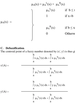
B. Triangular Membership functions.
A triangular membership function is represented by a triplet (a,b,c) as shown below:
0
if x < a
(x-a)/(b-a)
if b
≤ x ≤ c
Triangle(x:a,b,c) =
1
if x=b
(c-x)/(c-b)
if b
≤ x ≤ c
[image:4.595.61.539.52.285.2]where, a and c are upper bound and lower bound of the function, respectively. Setting up upper and lower bound values demands domain knowledge.
Let the membership function in the interval [a, b] be
denoted by μAL(x) and the membership function in the
interval [b, c] be denoted by μAR(x). Then,
μA(x) = μA
L(x) + μA
R(x)
μA
L(x)
if b
≤ x ≤ c
μA
(x) =
1
if x=b
μA
R(x)
if b
≤ x ≤ c
0
Otherwise
C. Defuzzification.
The centroid point of a fuzzy number denoted by (x', y') is thus given by, b b
∫ x μAL(x) dx + ∫ x μAR(x) dx
a a x'(A) =
b b
∫ μAL(x) dx + ∫ μAR(x) dx
a a
b b
∫ y μAL(x) dx + ∫ y μAR(x) dx
a a y'(A) =
b b
∫ μAL
(x) dx + ∫ μAR(x) dx a a
Rank of a fuzzy number is then given by,
R(A) = √ x'2 (A) + y'2(A)
D. Proposed Optimization Model
An optimization function subject to n constraints can be represented mathematically as
Maximize/Minimize f(xi)
subject to
gj(xi) <= C 1 ≤ j ≤ n Ṿ x ϵ X.
where, f(xi) is an objective function to be optimized and
gj(xi) are n constraints defined on the solution space Rn and
X = [x1, x2, x3, . . . . , xn]
The problem boils down to finding values xi ϵ Rn where 1 ≤ i ≤ n satisfying the constraints which optimize the objective function f. The problem can be stated as , Find the feasible point xi* in solution space Rn which satisfies all the
constraints for which f(x*) <= f(x) x.
Then, x* becomes an optimal solution.
E. Formulation of Non-linear Optimization Problem with Fuzzy Coefficients.
Maximize/Minimize f((xi), μ(xi))
subject to the constraints
gj((xi), μ(xi)) <= {Ci, μ(Ci)} 1 ≤ i ≤ m Ṿ x ϵ X.
X is a real valued vector given by,
X = [(x1, μ1), (x2, μ2), (x3, μ3), . . . . , (xn, μn)]
[image:5.595.34.297.104.467.2]F. Genetic Algorithm to Compute Membership of a Real Valued Vector.
6. NON-LINEAR FUZZY GA OPTIMIZATION
In literature, numerous techniques have been proposed for the solution of fuzzy linear and non-linear optimization problems, by ranking of fuzzy numbers by defining ranking functions, fuzzy linearly programming by defining parametric form for fuzzy numbers etc. Unlike linear programming, non-linear programming is convex in nature. Hence convex programming techniques can be adopted for solving non-linear optimization problems. In the case of non-convex nature of non-linear programs, it is difficult to search for exact global optimal solution. However, some approximate solution methods such as simulated annealing, genetic algorithm etc. can be employed for obtaining near optimal solutions. In the current study, genetic algorithm is employed for solving fuzzy non-linear optimization problem where coefficients of objective function and constraints are fuzzy in nature with triangular membership functions.
A. Fuzzy Ranking
A ranking function can be defined to provide a simple method for ordering fuzzy numbers.
B. Formulation of Fuzzy Non-linear Optimization Problem
In this section the model is proposed for the solution of non-linear optimization problem characterized by non-non-linear fuzzy objective function and non-linear fuzzy constraints. Consider the non-linear minimization problem subject to m constraints as shown below:
Minimize : z = f(xi)
subject to m constraints given by,
cj(xi) ≤ (≥) ai i=1, 2, 3, . . . , m.
The corresponding fuzzy version of the problem is Minimize : z = f(xi)
subject to m constraints given by,
cj(xi) ( ) ai i=1, 2, 3, . . . , m.
where, ~ notation is employed to denote fuzzification of crisp numbers.
Let the lower and upper bounds of the optimization values be represented by zl and zu, respectively,
Where,
zl = min {z1, z2} and
zu = max {z1, z2}.
z1 is given by
z1 = Minimize f(xi)
subject to m crisp constraints given by,
cj(xi) ≤ (≥) ai i=1, 2, 3, . . . , m, and x Rn
and x ≥ 0. and
Z2= Minimize f(xi)
subject to m crisp constraints given by,
cj(xi) ≤ (≥) ai + pi i=1, 2, 3, . . . , m, and x Rn
and x ≥ 0,
where pi is obtained by fuzzification of ai.
ai~ =
for triangular membership functions is given by,
ai ~
= =
0 x < bi-pi
bi-pi≤ x ≤ bi
bi≤ x ≤ bi+pi
[image:7.595.196.420.568.672.2]The triangular membership function is shown in Figure 3.
Figure 3. Structure of Triangular Membership Functions
C. Fuzzy Genetic Algorithm Applied to Line Balancing Problem
For the fuzzy variable xi [a, b] where a and b are lower and
upper limits of xi, respectively, a binary coding is employed
in order to generate an initial population. To achieve this a string Xi of length xi is randomly selected xi with
characteristic value of o or 1.The value of xi is computed
xi = ai + (bi-ai)
*
For a string of length 8, =8.
Employing fuzzy addition and fuzzy scalar multiplication, the left side of the constraint is computed. The fuzzy numbers so obtained are compared employing distance method. The fitness value of the function given by
where, is the objective value of population is computed for all members of the population. After computing fitness value of entire population, ranking is assigned to each member of the population based on fitness value and average fitness value is computed. The members from the current generation with the fitness value exceeding the average fitness value are selected in the mating pool for the next mating
Minimize :
=
Subject to the constraints
Lower bound , actual value and upper bound of the fuzzy coefficients of objective function
The algorithm employed for the solution is presented in the following section.
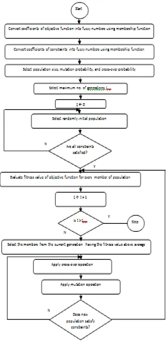
D. Algorithm for Fuzzy Non-Linear optimization Problem
An algorithm for solving fuzzy non-linear optimization problem using Genetic algorithm is given below:
1. Convert the coefficients of objective function and the coefficients of constraint functions into corresponding fuzzy numbers using triangular membership functions. Compute the lower and upper bounds of the optimal values employing the optimal value obtained in crisp optimization.
2. Calculate the objective function and left and right shape functions of the constraints using equations
3. Define the following parameters Population size
Mutation rate Selection rate Crossover points
Initial number of generations Maximum generations and No. of maximum iterations.
4. Encode the decision variables into binary strings of finite length.
5. For the current generated population, decode the values. If the current population satisfies all the constraints then go to step 6, otherwise goto step and repeat the procedure.
6. Compute the value of the objective function for each chromosome and compute fitness value given by equation
7. Perform the selection of mating parents employing the standard roulette wheel section method. The individuals with the best fitness values possess the higher probability of being selected in the next iteration and as such are selected for recombination.
8. Perform cross-over operation on selected members from the previous generation for yielding offsprings bearing resemblance to two parents.
9. Perform mutation operation which searches an entire search space for existence of global optimum.
7. CASE STUDY : JADHAV INDUSTRIES, KOLHAPUR
The theoretical model developed in section 3.4.3 has been applied for smoothening of production line at a small scale industry, Jadhav Industries, kolhapur which is one of the leading manufacturer and supplier of cast and machine ductile iron and gray cast iron components.
A. Company Profile
Jadhav industries, situated in Kolhapur, supplies auto components to Ashok Leyland, Kirloskar Oil Engines Ltd., John Deere, Greaves Cotton Ltd., Mahindra and Mahindra, Piaggio Vehicles and Tecumesh. It is one of the leading manufacturer and supplier of cast and machined ductile iron, and gray cast iron components. Company is specialized in supply of automotive components and within a span of two decades the company has crossed a turn over of 130 crore rupees per annum. The company is well known for its quality standards and dedicated to fulfill the stringent customer requirements. The company employs process of on-going improvements to manage production line for optimal lead time and is having ISO-9000:2008 certification.
B. Problem Definition
non-dependent resource information, and other important parameters are in XML format along with their document type definitions (DTD).
C. Crisp and Fuzzy Non-Linear Optimization of Total Cost of Housing Production Line of Jadhav Industries
[image:9.595.54.538.169.267.2]The models proposed above are implemented in Evolutionary solver and MatLab, respectively. Lower bound , actual value and upper bound of the fuzzy coefficients of objective function are illustrated in Table 1.
Table 1. Representation of Fuzzy Numbers
Fuzzy Number Lower Limit Actual Number Upper limit
400 410 420
3 4 5
7 8 9
8 9 10
9 10 11
10 11 12
11 12 13
Number of parts is set to 10.
In the current study, binary strings of length 10 are employed. Roulette-wheel selection procedure is adopted. Single point cross-over operation bitwise mutation operator are employed. The crossover probability is fixed at 0.7 and
mutation probability is set to 0.6. The initial population size is set to 10 and maximum number of iterations is set to 1000. The initially randomly generated population is shown in Table 2.
Table 2. Initial Randomly Generated Population
X1 X2 X3 X4 X5 X6 X7
1001111001 1010100001 0111111001 1000101101 1010100000 1010101000 1000010110 1001111101 1000001111 1010011101 1011001000 1001100110 1010100101 1000111011 1010101010 0111110100 1001111111 0111111011 1010100111 1001011111 1010001100 1011011110 0101011110 0111001010 1100010101 1101011000 0110010011 1010000000 0110001001 1011000100 1110111000 1000110101 1100000110 0111100110 1110100101 0101101010 1001100110 0101101110 1110100010 1000110001 1000101101 1010100000 1010101010 0111110100 1010000000 0110001001 0101101110 1110100010 1010101010 1100000110 1000111011 1010101010 0111110100 1001111111 0101101010 1001100110 0101101110 1110100010 1010000000 0110001001 0101101010 1001100110 1010100101 1000111011 1100010101 1101011000 0101101110 1110100010 1010101000 0110001001
After substituting the values in the objective function and determining the fitness value for each member of the population, the members from the previous population having fitness value exceeding average fitness value with frequency of repetition based on ranking generated by roulette wheel selection are adopted and proceed to the next
generation. After selection, the cross-over operation and mutation operation are applied. Population after cross-over operation and mutation operation are presented in Table 3 and Table 4, respectively.
Table 3. Population After Cross-Over
X1 X2 X3 X4 X5 X6 X7
Table 4. Population After Mutation
X1 X2 X3 X4 X5 X6 X7
1001111001 1001111111 1010110111 1011100000 1111111101 1000000011 0000110001 1000111001 1000000110 1000101000
1011100000 1111111101 1000000011 1000101000 1110100101 1110100000 0111110100 1001001010 1001111000 1000111011
1011111011 1011001010 1000100111 1010010101 1110001001 0010100100 0111101100 0011010110 0001000010 0010110101
1010010101 1110001001 0010100100 0010110101 1010010001 0011011000 0001000111 0011010010 0001101001 0011001010
0001101001 0011001010 1101000010 0100011111 0100000101 1001100101 1001000101 1011011011 1011001001 1111101111
1000101000 1110100101 1110100000 0111110100 1001001010 1110001001 0010100100 0010110101 1010010001 0011011000
1000000011 1000101000 1110100101 1111111101 1000000011 0000110001 1000111001 0011011000 0001000111 0011010010
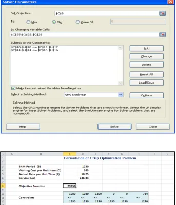
Both the crisp and fuzzy optimization models are implemented and are compared. Figure 4(a) depicts the
implementation of crisp model where the optimal value is found to be 29256 units.
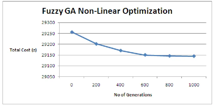
The model is executed for different generations and membership functions and = 0.5 provides best results for different generations. The results of Z obtained for 5 runs
with the grade of the membership function set at = 0.5 are depicted in the Figure 4(b) with the value of z corresponding to zero generation signifying crisp value.
Figure 4(b). Execution of Fuzzy Non-linear GA Optimization Model for Different Generations.
It is evident from the Figure 4(b) that the z value converges for no of generations > 800 with the optimal value given by 29144 as against crisp optimum value of 29256. Owing to the nature of cost function there is no drastic change in the optimal values computed employing crisp and Fuzzy-GA
[image:11.595.88.507.114.322.2]optimization techniques. The search space contains a single prominent minimum. The relative comparison of the results obtained in the two cases is depicted in Table 5.
Table 5. Relative Comparison Between Crisp and Fuzzy-GA Optimization Results
w1 w2 w3 w4 w5 w6 w7 Total Cost Crisp Optimization 0 0 0 14 8 0 0 98 29256 Fuzzy-GA Optimization 0 0 0 13 8 0 0 96 29144
8 CONCLUSION AND SCOPE FOR FUTURE WORK
In the current research, the authors have designed a model for both crisp and fuzzy optimization for production line balancing problem and have applied nonlinear fuzzy-GA optimization model for solving production line balancing problem of Jadhav Industries Pvt. Ltd, Kolhapur. The algorithm for fuzzy non-linear optimization using Genetic Algorithm is presented. At the outset the conceptual model is implemented in Excel using simulation technique and GRG Non-linear engine for solver problem to derive the first hand information and the same is utilized to fine tune the optimization algorithm using Fuzzy-GA technique. Triangular membership functions are utilized for modeling fuzzy numbers. Defuzzification process is based on center of gravity. The model is executed for different generations and membership functions and = 0.5 provides best results for different generations. The z value corresponding to total cost converges for no of generations > 800 with the optimal value given by 29144 as against crisp optimum value of 29256. Owing to the nature of cost function there is no drastic change in the optimal values computed employing crisp and Fuzzy-GA optimization techniques. The search space contains a single prominent minimum. The work can
be extended to explore the nature of different membership functions.
REFERENCES
[1]. NimaHamta, S.M.T. FatemiGhomi, M. Hakimi-Asiabar, P. HooshangiTabrizi, “Multi-objective Assembly Line
[2]. Balancing Problem with Bounded Processing Times, Learning Effect, and Sequence-dependent Setup Times”, 978-1-4577-0739-1/11, IEEE, 2011, pp. 768-772.
[3]. Chung-Jen Kuo, Chih-Ming Liu, Chih-Yang Chi, “Standard WIP Determination and WIP Balance Control with Time Constraints in Semiconductor Wafer Fabrication”, Journal of Quality, vol. 15, no. 6, 2008, pp. 409-420.
[4]. Rasaratnam Logendran, Paula deSzoeke, Faith Barnard, “Sequence-dependent group scheduling problems in flexible
flow shops”, Int. J. Production Economics, vol. 102, 2006 ,
pp. 66–86.
[5]. Isabel C. PraGa, Marina del Rey, “An approach for Manual Production Lines Balancing, SimBa”, Proceedings of the 1997 IEEE International Symposium on Assembly and Task Planning CA -, August 1997, pp. 42-47.
[6]. PEI Ling, LI Feng, LIN Fuquan, WANG Wei, “Case Study for Integrating the Line Balancing and the Shop Layout Based on Autocad”, pp 1-5.
[image:11.595.64.537.440.481.2][8]. D. Roy and D. Khan, “Assembly line balancing to minimize balancing loss and system loss”, J. Ind. Eng. Int., vol. 6, no. 11, pp. 1-5, Spring 2010 ISSN: 1735-5702 © IAU, South Tehran Branch
[9]. Ali A.J. Adham and Razman Bin Mat Tahar, “Optimum efficiency of production line in automobile manufacture”, African Journal of Business Management, vol. 6, no. 20, May 2012, pp. 6266-6275.
[10].Hung-Nan Chen and Jeffery K. Cochran, Effectiveness of Manufacturing Rules on Driving Daily Production Plans”, Arizona, Journal of Manufacturing Systems, vol. 24, no. 4., 2005, pp. 339-351.
[11].Nils Boysen , Malte Fliedner , Armin Scholl, “A classification of assembly line balancing problems”, European Journal of Operational Research, vol. 183, 2007, pp. 674–693.
[12].Cheng-Hung Wu, James T. Lin , Wen-Chi Chien, “Dynamic production control in parallel processing systems under process queue time constraints”, Computers & Industrial Engineering, vol. 63, 2012, pp. 192–203.
[13].Andreas C. Nearchoun, “Maximizing production rate and workload smoothing in assembly lines using particle swarm optimization”, Int. J. Production Economics, vol. 129, 2011, pp. 242–250.
[14].Christian Becker, Armin Scholl, “A survey on problems and methods in generalized assembly line balancing”,
European Journal of Operational Research, vol.168., 2006, pp. 694–715.
[15].HadiGo¨kc,en ,Ku¨rs_adAgˇpak, “A goal programming
approach to simple U-line balancing problem”, European Journal of Operational Research, vol. 17, 2006, pp. 577–585. [16].Hadi Go¨ kc-en, Ku¨ rs-ad Ag˘pak, RecepBenzer, “Balancing
of parallel assembly lines”, Int. J. Production Economics, vol. 103, 2006, pp. 600–609.
[17].M. A. Hannan, H.A. Munsur, M. Muhsin, “An Investigation of the Production Line for Enhanced, Production Using
Heuristic Method, International Journal of Advances in Engineering & Technology, Nov 2011, pp. 77-88.
[18].Lale Ozbakir, Adil Baykasoglu, Beyza Gorkemli, Latife Gorkemli, “Multiple-colony ant algorithm for parallel assembly line balancing problem”, Applied Soft Computing, vol. 11, 2011, pp. 3186–3198.
[19].Armin Scholl , Christian Becker, “State-of-the-art exact and heuristic solution procedures for simple assembly line balancing”, European Journal of Operational Research, vol. 168, 2006, pp. 666–693.
[20].Lui Wen Han Vincent and S. G. Ponnambalam, “A Differential Evolution-Based Algorithm to Schedule Flexible Assembly Lines”, IEEE Transactions On Automation Science And Engineering, vol. 10, no. 4, October 2013, pp. 1161-1165.
[21].Lixin Tang, and Xianpeng Wang, “A Scatter Search Algorithm for a Multi stage Production Scheduling Problem With Blocking and Semi-Continuous Batching Machine”, IEEE Transactions On Control Systems Technology, vol. 19, no. 5, September 2011.
[22].Christos Dimopoulos and Ali M. S. Zalzala, “Recent Developments in Evolutionary Computation for Manufacturing Optimization: Problems, Solutions, and Comparisons”, IEEE Transactions On Evolutionary Computation, vol. 4, no. 2, July 2000, pp. 93-110.
[23].XU Weida , Xiao Tianyuan Tsinghua, “Strategic Robust Mixed Model Assembly Line Balancing Based on Scenario Planning”, Science And Technology, vol. 16, no. 3, June 2011, pp 308-314.