CubeSats for System Evolvability: A Case Study.

(1)

ABSTRACT

LAWRENCE, CHARLOTTE ANNE. CubeSats for System Evolvability: A Case Study (Under the direction of Dr. Scott Ferguson and Dr. Mark Pankow.)

(2)

(3)

CubeSats for System Evolvability: A Case Study

by

Charlotte Anne Lawrence

A thesis submitted to the Graduate Faculty of North Carolina State University

in partial fulfillment of the requirements for the Degree of

Master of Science

Aerospace Engineering

Raleigh, North Carolina 2017

APPROVED BY:

_________________________ _________________________ Dr. Andre Mazzoleni Dr. Mark Pankow

Co-Chair of the Advisory Committee

_________________________ Dr. Scott Ferguson

(4)

ii

DEDICATION

(5)

iii

BIOGRAPHY

(6)

iv

ACKNOWLEDGEMENTS

The author would like to express her appreciation for her advisors Dr. Scott Ferguson and Dr. Mark Pankow, who went above and beyond in their support over the past two years. The author would also like to thank her lab-mates Gordon Beverly III, Krista Edwards, Anya Flowe, Rachel Hough, Daniel Long, Jaekwan Shin, Samantha White, and Kevin Young for their assistance and support during her tenure in the System Design Optimization Lab.

(7)

v

LIST OF TABLES

Table 2.1 - FireSat II Mission Objectives [31] ... 13

Table 2.2 - The 2 Principal Options for FireSat II [50] ... 13

Table 2.3 - Targeted Mission Requirements [28,31] ... 16

Table 2.4 – CubeSat Sizes and Corresponding Dimensions [28] ... 17

Table 2.5 – Commercially available CubeSat Structures [57,58] ... 18

Table 2.6 – ADC Design Drivers ... 20

Table 2.7 – Possible Reaction Wheels [67,69] ... 25

Table 2.8 – Possible Magnetic Torquers [68,70,71] ... 25

Table 2.9 – Possible Antennas [74,75] ... 27

Table 2.10 – CubeSat Sun Sensor Options ... 30

Table 2.11 – Sample CubeSat Horizon Sensors ... 30

Table 2.12 – ISIS Full Ground Station Packages for Purchase [82] ... 36

Table 2.13 – A sample of batteries found on CubeSatShop [89–91] ... 37

Table 2.14 – Center of Mass Requirements [28] ... 45

Table 2.15 – Solar Panels available for CubeSat Use [94–96] ... 46

Table 3.1 – FireSat II Mission Objectives [31] ... 53

Table 3.2 – FireSat II Mission Requirements Driving the creation of the Mathematical Model 54 Table 3.3 - Variables and their Ranges relating to the Ground Sample Distance Model ... 60

Table 3.4 – Variables and their Ranges relating to the Camera Size Model ... 62

Table 3.5 – Satellite Lifespan Estimates [51] ... 65

Table 3.6 – Calculated Altitude Ranges ... 67

Table 3.7 – Lifespan Ranges ... 67

Table 3.8 – Orbital Lifespan as a Function of CubeSat Size and Time Step ... 68

Table 3.9 – Variables and their Ranges relating to the Orbit Model ... 68

Table 3.10 – United States Launch Locations and Resulting Inclinations ... 70

Table 3.11 – Variables and their Ranges relating to the Ground Track Model ... 72

Table 3.12 – Variables and their Ranges relating to the Swath Width Model ... 74

Table 3.13 – Variables and their ranges used in the System Model ... 76

Table 3.14 – Variables included in the Design String... 77

Table 3.15 – Subsystem Cost Approximations ... 79

(10)

viii

Table 3.17 – Cost Data Provided from FLIR Representative ... 81

Table 3.18 – Pixel Pitch Cost Model ... 82

Table 3.19 – Explanation of the types of Costs associated with Wildland Fires [106] ... 88

Table 3.20 – Latitudes and Longitudes of NOAA Ground Stations ... 92

Table 3.21 – Direct Relationships between the Mathematical Model and the Subsystem Factors and Drivers ... 98

Table 4.1 – Driving Mission Requirements for the One Year Mission ... 103

Table 4.2 – Results from the One Fire Season Mission ... 104

Table 4.3 – Eight Year, Single Design Mission ... 114

Table 4.4 – Results from the Eight Year, Single Satellite Mission ... 114

Table 4.5 – Cameras Used for the Eight Year, Single Satellite Mission ... 121

Table 7.1 – Level 0 Mission Requirements... 140

Table 7.2 – Level 1 Mission Requirements ... 141

(11)

ix

LIST OF FIGURES

Figure 1.1 – Acres Burned and Number of Fires since 1960, data supplied by the National

Interagency Fire Center [33] ... 5

Figure 1.2 – Fire Season Length [40] ... 6

Figure 2.1 – System Map from Space Mission Engineering ... 10

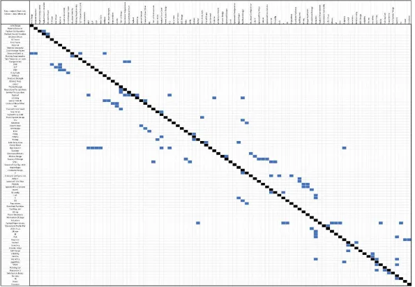
Figure 2.2 – Design Structure Matrix created based on the Drivers and Factors presented in Space Mission Engineering ... 12

Figure 2.3 - Propulsion Subsystem Drivers ... 14

Figure 2.4 – Simplified Propulsion Subsystem Drivers... 15

Figure 2.5 –Final Map of Propulsion Subsystem Drivers ... 20

Figure 2.6 – ADC Design Drivers ... 22

Figure 2.7 – Simplified ADC Subsystem Drivers ... 23

Figure 2.8 – Final Map of ADC Subsystem Drivers ... 31

Figure 2.9 – CDH Design Drivers ... 32

Figure 2.10 – Simplified CDH Design Drivers ... 32

Figure 2.11 – Final Map of the CDH Subsystem... 34

Figure 2.12 – TTC Design Drivers ... 35

Figure 2.13 – Simplified TTC Design Drivers ... 35

Figure 2.14 – Final Map of the TTC Subsystem ... 38

Figure 2.15 – Power Design Drivers ... 39

Figure 2.16 – Simplified Power Design Drivers ... 40

Figure 2.17 – Percent of orbital period when a LEO satellite would be in Earth’s Shadow ... 41

Figure 2.18 – Final Map of the Power Subsystem ... 42

Figure 2.19 – Mechanical Design Drivers ... 43

Figure 2.20 – Simplified Mechanical Subsystem Design Drivers ... 44

Figure 2.21 – Final Map of the Mechanical Subsystem ... 47

Figure 2.22 – Thermal Subsystem Design Drivers ... 48

Figure 2.23 – Simplified Thermal Subsystem Drivers ... 49

Figure 2.24 – Final Subsystem Map for the Thermal Subsystem ... 50

Figure 2.25 – DSM of Final Driver and Factor Breakdown ... 51

Figure 3.1 – Number of Cameras which can achieve the desired GSD at a given altitude ... 56

(12)

x

Figure 3.3 – Possible Ground Sampling Distances ... 57

Figure 3.4 – Potential GSDs below 50m2_{... 58}

Figure 3.5 – Lens Diameters required to meet 50m2_{for a given altitude ... 59}

Figure 3.6 – Mass of the Total Camera Assembly as a Function of Lens Diameter ... 61

Figure 3.7 – Lens Length as a Function of Lens Diameter ... 62

Figure 3.8 – Visual representation of the Orbit Model... 65

Figure 3.9 – Maximum Lifespans as a function of initial altitude and CubeSat size, highlighting the intersection of the lifespans and maximum altitude ... 66

Figure 3.10 – Minimum Lifespans as a function of initial altitude and CubeSat size, highlighting the intersection of the lifespans and minimum altitude ... 66

Figure 3.11 – Visual representation of the ground track model used ... 69

Figure 3.12 – Differences in Fidelity of the Ground Track Model based on Time Step ... 71

Figure 3.13 – Swath Width [62] ... 72

Figure 3.14 – Visual Representation of the Instrument Swath Width Model Used ... 73

Figure 3.15 – Overall System Model ... 75

Figure 3.16 – Design String... 78

Figure 3.17 – Cost Model for Pixel Pitch ... 82

Figure 3.18 – Cost Model of Lens based on Effective Focal Length ... 83

Figure 3.19 – Cost Combinations ... 84

Figure 3.20 – Camera Resolution Trends over time ... 85

Figure 3.21 – Camera Cost over time ... 85

Figure 3.22 – Cost per Megapixel of Resolution in digital cameras over time ... 86

Figure 3.23 – Suppression Costs per Acre over the last 32 years [107] ... 89

Figure 3.24 – Distribution of Acres Burned per Fire [107] ... 89

Figure 3.25 – Distribution of the number of Nevada Fire Starts per day in the last 15 years ... 90

Figure 3.26 – NOAA LEO Ground Stations [122] ... 91

Figure 3.27 – Logic for Determining the Penalty Function for Mission Life ... 93

Figure 3.28 – Coverage Penalty Function Formulation ... 95

Figure 3.29 – Camera Mass as a Function of Lens Diameter ... 95

Figure 3.30 – Camera Volume as a Function of Lens Diameter ... 96

Figure 3.31 – Objective Function Flow... 101

(13)

xi

Figure 4.2 – Launch Altitudes, Size and Resulting Altitudes as a function of time for a One Fire

Season Mission ...106

Figure 4.3 – Box and Whisker Plot representing the resulting Launch Altitudes for a One Fire Season Mission ... 107

Figure 4.4 – Box and Whisker Plots of the resulting orbital parameters for a One Fire Season Mission ... 107

Figure 4.5 – Example Coverage Count for a One Fire Season Mission ...109

Figure 4.6 – Sample Daily Passes through the Target Location ...109

Figure 4.7 – Ground Sample Distances for a One Fire Season Mission ... 111

Figure 4.8 – Distribution of Effective Focal Lengths for the One Fire Season Mission ... 112

Figure 4.9 – Example Convergence plots for Trial 7, the cheapest solution... 117

Figure 4.10 – Comparison of the Launch and Orbit Patterns of the resulting mission profiles from the Eight Year, Single Design Mission ... 118

Figure 4.11 – Box and Whisker Plot representing the resulting Launch Altitudes for the Eight Year, Single Design Mission ... 119

Figure 4.12 – Example Coverage Count for an Eight Year, Single Design Mission ... 120

Figure 4.13 – Ground Sample Distances for the Eight Year, Single Design Mission... 122

Figure 5.1 – Final System Map... 126

Figure 5.2 – Final System Design Structure Matrix ... 127

Figure 5.3 – Objective Function Formulation ... 128

(14)

xii

LIST OF SYMBOLS, ABBREVIATIONS AND NOMENCLATURE

Table of Variables

Symbol Variable Value Usage

𝐴𝑟 Cross-sectional area in the Ram Direction

-- (4)

𝐴𝑠 Surface Area the Sunlight is impacting -- (5)

B Magnetic Field Strength -- (2),(3)

𝐶𝑑 Drag Coefficient -- (4)

c Speed of Light

𝑐𝑝𝑎 Center of Aerodynamic Pressure -- (4)

𝑐𝑝𝑠 Center of Solar Radiation Pressure -- (5)

𝑐𝑚 Center of Mass of the Spacecraft -- (4)

D Spacecraft’s Residual Dipole Moment -- (2)

𝐼𝑥, 𝐼𝑦, 𝐼𝑧 Moments of Inertia -- (1),(6)

𝑖𝑠 Inclination Angle of the Sun onto the orbital plane

(7) M Magnetic moment of the earth

multiplied by the magnetic constant

(3)

𝑚𝑖 Mass of the ith component -- (6)

P Orbital Period -- (9)

q Unitless reflectance factor -- (5)

𝑅 Radius of the Spacecraft (1),(3)

𝑅𝐸 Radius of the Earth (7)

𝑟𝑖 Perpendicular distance of the ith component’s center of mass to the

designated axis

(6)

𝑡𝑆𝐻 Time in Shadow -- (9)

V Orbital Velocity -- (4)

θ Angle between local vertical and principal Z axis

-- (1)

𝜃𝐸 Eclipse Angle -- (8),(9)

𝜃𝐺 Geocentric angle -- (7),(8)

λ “unitless function of the magnetic latitude that ranges from 1 at the magnetic equator to 2 at the magnetic

poles”

(3)

µ Earth’s Gravitational Constant (1)

ρ Atmospheric Density -- (4)

𝜏𝑎 Atmospheric Drag Torque -- (4)

𝜏𝑔 Gravity Gradient Torque -- (1)

𝜏𝑚 Magnetic Field Torque -- (2)

𝜏𝑚 Solar Radiation Pressure Torque -- (5)

Φ Solar Constant (5)

(15)

1

1 INTRODUCTION

Complex engineered systems have a large number of components whose overall structure and behavior is [1] the direct result of the interactions of their components. [2] Additionally, the response of system components change according to their interactions with neighboring components [1]. However, as systems become more complex, there is a greater chance of component failure, resulting in decreased performance or loss of function [3]. In this thesis, a monolithic (integral) architecture will be decomposed into a series of distributed (modular) systems in an attempt to both reduce cost and meet the same initial mission requirements while exhibiting the ability to respond to mission changes.

1.1 Background

In software engineering, a system is considered monolithic if its distinguishable aspects are interwoven [4], and a system is considered distributed if the distinguishable aspects are self-contained [5]. When applying this concept to engineering design and complex engineered systems, integral systems have one function that is realized by many different, connected, components [6]. A modular system is a system in which each component has one particular function [6]. According to Hölttä-Otto and de Weck, a module is “commonly defined as an independent chunk that is highly coupled within, but only loosely coupled to the rest of the

system” [7].Modular systems can exhibit varying degrees of modularity [7–9], requiring

advanced planning and forethought to determine proper module combinations, understand module interactions and the optimal degree of modularity.

(16)

2

engineered system do not have the benefit of organically evolving over thousands of generations, and must be strategically designed to handle these changes.

Previous work has determined that evolution capacity of a complex engineered system was directly related to the excess present in the system. In this excess is defined as the surplus in components or systems once the requirements of the component or system are met. [12] Evolvability allows a system to adapt to new situations. To facilitate this ability, the system should possess standard electrical and mechanical interfaces, an open control structure, and the ability to develop past the original intent of the system. [13] Many of these system facilitators are reminiscent of defining features found in modular architectures.

Traditionally, aerospace systems are designed with weight, safety, cost and reliability as driving influences, resulting in an integral architecture [8,14]. By using integral architectures, aerospace systems generally include higher interaction density and a hierarchical architecture of components, both of which have been shown to limit the evolutionary capability of the system. [15] Previous groups have explored the idea of modular satellites [16–21] with limited success, as their programs died in infancy [16,19,20]. Traditional, integral, satellites are time and cost intensive; it can take years to develop, test, certify, and launch a system. Often, by the time a traditional satellite is launched, the technology on board is out of date, yet there is not enough time or money to certify the new technologies and update the system designs without entering a vicious cycle and delaying launch indefinitely. Creating modular, easy to evolve systems would mean that designers could replace and update their systems in pieces rather than in large, slow, and expensive system overhauls. This has the potential to revolutionize design and innovation of the space industry, as, program directors and/or consumers would be more willing to take risks on new technology if costs decreased. Previous groups have explored the idea of non-traditional satellites architectures with limited success.

(17)

3

Realizing the scientific benefits of small satellites requires the reconsideration of design strategies for creating satellite clusters.

The interfaces between the satellites in a swarm are not the only paradigm that must be challenged. A little over a decade after Hurricane Katrina, NASA launched the Cyclone Global Navigation Satellite System (CYGNSS). CYGNSS consists of eight microsatellites (approximately 75 lbs. each) capable of creating images of wind speed intensities and storm surges every few hours [18,19]. Effectively the size of a suitcase, this reduction in satellite size was achieved by using reflected ocean surface roughness signals from the GPS system, rather than having the CYGNSS satellites sense this information. However, while there is a functional decoupling in the mission design, each satellite in the cluster is self-contained – each contains its own power, navigation, propulsion, and sensor packages tied into a central bus architecture. The CYGNSS system is also designed to be launched from a Pegasus XL rocket, as it is too large for existing CubeSat launchers. [24] Pursuing design solutions that can be put into orbit using CubeSat launchers could lead to substantial cost savings and easier orbital access. In the ten years it took to design and launch the CYGNSS system, the United States experienced three additional hurricanes that ranked among the top 5 costliest hurricanes in United States History – amounting to $121.5 billion dollars in damages. [25]

Operationally Responsive Space (ORS) is an Air Force satellite architecture designed for rapid responses. By using plug and play, bus-based architectures, the Air Force is exploring how to decrease design time allows for the ability to create a set of satellites which can be designed and launched quickly to respond to changing needs [20]. The program aims to integrate military capability with networked, autonomous, rapidly produced satellites. The goal of this design is not optimization but agility and dynamic fitness [20]. ORS allows for the construction of a satellite in a few short hours. However even ORS cannot avoid the high cost of launch. Test satellites are around 450 kg, mandating primary payload status and an inherently expensive launch cost [26].

(18)

4

to launch their own satellite. Civil, commercial, military, and university developers have all launched CubeSats since 1999 [29], and are continuing to do so and as technology improves, so to do the capabilities of the CubeSats designed and launched. [29] Still a popular architecture, with CubeSat deployments attached to launches through Spring of 2018 [30], CubeSats are self-contained modules that can be combined to form a larger system. This work will use the CubeSat architecture and a sample mission to determine potential performance gains by using this modular architecture in place of a traditional monolithic architecture.

1.2 Selection of FireSat II as a Case Study

When determining the sample mission for the case study examined in this work, two factors were considered: value of mission and level of detail to compare with. FireSat II was selected as the Case Study for this thesis because it met both of these factors. FireSat II is an example mission in Space Mission Engineering: The New SMAD, a popular text for those who want to learn about aerospace engineering and aerospace system design. As an example mission, FireSat II has defined mission objectives and requirements to which the proposed alternatives could be compared. With its primary mission objective being to “… detect, identify, and monitor forest fires throughout the United Sates, including Alaska and Hawaii, in near real time and at a low cost,” [31] FireSat II provides the opportunity for genuine scientific merit. By selecting a well-documented mission like FireSat II there is ample information for system architecture level comparisons.

(19)

5

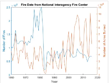
Figure 1.1 – Acres Burned and Number of Fires since 1960, data supplied by the National Interagency Fire Center [33]

Anthropogenic climate change has been identified as one of the driving factors increasing the total area of acres burned. “Climate change contributes to forest fires in a number of ways. Fires kill off trees and other plants that eventually dry and act as the fuel to feed massive wildfires. Global warming also increases the likelihood of the dry, warm weather in which wildfires can thrive.”[32] Global warming increases wildfire risk in four ways: longer fire seasons, drier conditions, more fuel for forest fires, and increased frequency of lightning. [34,35] This past year, 2016, was the warmest year on record since the National Oceanic and Atmospheric Administration (NOAA) began tracking global temperatures 137 years ago. It is also the third year in a row that the most recent year has surpassed the previous as the warmest year on record [36].

(20)

6

tactics, these areas are building up more dry fuel which later fuels even larger fires [38–40]. And thus, by over regulating the forest fires the number and severity of fires has increased [37]. Additionally, humans are the initial cause of 84% of wildfires while lightning only started the remaining 16%. [37] Additionally, fire season is extended by 50 days when human fires considered, [37] thus increasing both the length and severity of the each fire season. Fire season length in a region is defined by the date of the first fire discovery to the date of the last control of a fire. Since 1973, fire season length in the Western United States has increased from 138 days to 222 days. The first discovery of a fire has moved 34 days earlier, and the last controlled fire has occurred 50 days later than average. [40] Figure 1.2 below illustrates the changes in fire season length over time where the length of the fire season is defined as the difference between the first discovery day and the last control day.

Figure 1.2 – Fire Season Length [40]

With fires starting earlier and ending later, there is great cause for identification and tracking on fires as we move toward longer and more intense seasons. Thus, FireSat II not only provides enough information for system comparison but also provides environmental information with the potential for genuine impact.

This work will look at the FireSat II mission and design a modular system using the CubeSat architecture to meet the same mission requirements. By using a well characterized earth based imaging mission as the test case, this not only provide objectives for a mission, but it also provides a baseline for system architecture comparison for a thorough examination of the benefits and drawbacks of such a system.

1.3 Research Question

(21)

7

system characteristics required to decompose a monolithic architecture into a series of distributed systems in order to monitor forest fires by considering the following research question.

Using the CubeSat architecture as the framework for this mission, a model will be generated to determine potential performance gains by using this modular architecture in place of a traditional monolithic architecture proposed in Space Mission Engineering. By selecting a well-documented mission like FireSat II there is ample information for system architecture level comparisons as well as previous iterations of the FireSat design by which the capacity for evolvability for the proposed system can be examined.

Through this research question, a mathematical model of a CubeSat capable of meeting the system requirements of FireSat II will be created. Using this model, potential evolutions can be explored by manipulating the requirements placed on the system.

1.4 Summary of Chapters

The rest of the work done for this thesis is broken down into 4 additional chapters. Chapter 2 decomposes the satellite into its subsystem and identifies the important aspects for creating a mathematical model. Chapter 3 develops the components of the mathematical model and then combines them for evaluation through the use of a genetic algorithm and penalty functions. Chapter 4 implements the model developed in Chapter 3 and examines the implications of manipulating the requirements. And Chapter 5 concludes the research presented in this thesis and provides direction for future work on this topic.

(22)

8

2 SYSTEM DECOMPOSITION

Decomposing complex engineered systems can be a finicky task; determining how and why to divide a system into different subsystems can be frustrating and time consuming and a variety of methods [7,41–43] have been developed to assist in understanding the relationship between different system components. Even with a (relatively) common system like a satellite, different entities define the subsystems in different ways [44–49]. One common breakdown of a satellite results in six subsystems [47]:

• Attitude and Orbit Control System (AOCS) – containing Propulsion, Guidance, Navigation, and Control (GNC), and Attitude Determination and Control (ADC) • Command and Data Handling (CDH)

• Telemetry, Tracking and Command (TTC) • Structure and Mechanism (MECH)

• Power • Payload

Another breaks the satellite down into seven subsystems [49]: • Propulsion,

• Attitude Determination and Control (ADC) • Command and Data Handling (CDH) • Telemetry Tracking and Command (TTC) • Power

• Mechanical • Thermal

(23)

9

(24)

10

(25)

11

(26)

12

(27)

13

As discussed in Chapter 1, FireSat II was chosen as the case study by which a system model was developed because the details of all the subsystems are readily available, as well as the potential for genuine scientific merit regarding wildland fires in the United States. The primary and secondary mission objectives are presented in Table 2.1 below.

Table 2.1 - FireSat II Mission Objectives [31] Primary Mission Objective

To detect, identify, and monitor forest fires throughout the United Sates, including Alaska and Hawaii, in near real time and at a low cost

Secondary Mission Objectives

To demonstrate to the public that positive action is underway to contain forest fires To collect statistical data on the outbreak and growth of forest fires

To monitor forest fires for other countries To collect other forest management data

The options hypothesized in [50] as possible solutions are presented in Table 2.2 below. Table 2.2 - The 2 Principal Options for FireSat II [50]

Element FireSat II

Option A Option B

Mission Concept

Automated fire detection on board the

spacecraft with direct downlink

Manual fire detection at the ground station with results

relayed via FireSat II

Subject Heat from forest fire

Payload Small-aperture IR Large-aperture IR

Spacecraft Bus Small, 3-axis, Earth-pointing

Mid-large size, 3-axis, Earth-pointing

Launch System Small launch vehicle Large launch Vehicle

Orbit LEO, 2 satellites, 55

degrees

GEO, 1 satellite centered over the west coast of the U.S.

Ground System Single, dedicated ground station

Communications Architecture

TDRS data downlink; commercial links to

users

(28)

14

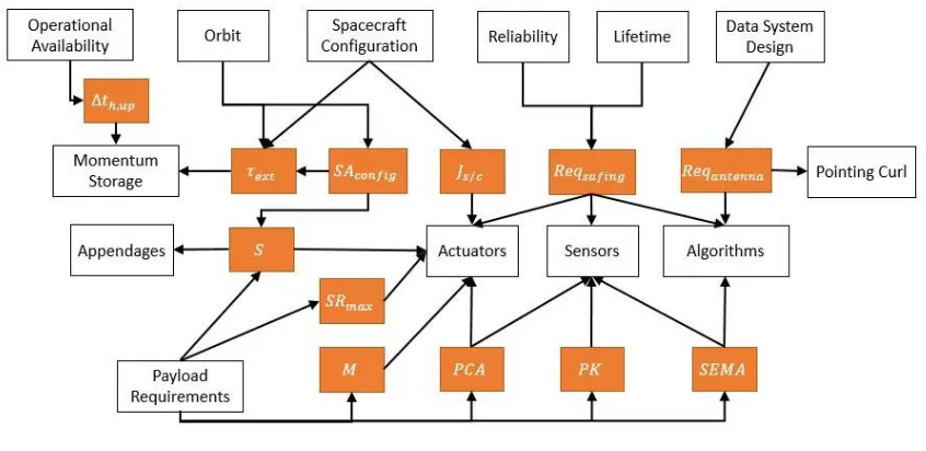
(LEO) which are defined as orbits that are less than 3,000 km [52] while Options B posits geosynchronous (GEO) orbits which occur at 35,856 km [52]. From this, the average CubeSat orbit more closely aligns with LEO orbits. Additionally, small-aperture IR cameras can be purchased as commercial off the shelf products [53] while large-aperture IR cameras are customized. Using this subsystem breakdown as a framework, each of the following sections explains the principal drivers and factors of the given subsystem and simplifies the subsystem with the modeling assumptions made. Each section also contains visual representations of the drivers, factors, and interactions, where drivers are represented by solid color blocks and factors are white boxes.

2.1 Propulsion Design Drivers and Factors

The three main drivers presented for the propulsion subsystem are: “Delta V” (∆𝑉), “Spacecraft Dry Mass” (𝑀𝑠 𝑐⁄ ,𝑑𝑟𝑦), and “Thrust for Maneuvers and Control” (𝑇𝑡𝑜𝑡𝑎𝑙). “Delta V” is defined as the total change in velocity required throughout the mission lifespan. [54] “Spacecraft Dry Mass” is the mass of the spacecraft before loading any propellants [55], and “Thrust for Maneuvers and Controls” is the total amount of thrust need through the mission lifespan to properly maneuver and control the spacecraft. These three drivers are initially related to six factors: “Mission Design,” “Spacecraft Design,” “Trajectory,” “ADC (Attitude Determination and Control) Design,” “Fuel Required,” and “Thruster Sizing.” The relationships between the subsystem factors and drivers are illustrated in Figure 2.3 below.

Figure 2.3 - Propulsion Subsystem Drivers

(29)

15

increases the regulations and restricts the number of launches in which the system is an eligible secondary payload. [28] Despite the decision to forgo the inclusion of any propellant in the design of this mission, the Propulsion Subsystem remains a subsystem because of the potential for the addition of a propulsion system in other CubeSat missions. Considering these regulations and restrictions, the map for the propulsion subsystem can be simplified to Figure 2.4.

Figure 2.4 – Simplified Propulsion Subsystem Drivers

In performing initial simplifications the “Thrust for Maneuvers and Control” and “Delta V” drivers of the system were eliminated. Also, the three factors associated solely with these drivers – “Fuel Required”, “Thruster Sizing”, and “Attitude Determination and Control (ADC) Design” – do not need to be considered in this subsystem map. Additionally, the “Trajectory” factor was combined with the “Orbit” factor to streamline vocabulary as orbit, not trajectory, is the vernacular used with satellites.[56] Another change was the addition of a connection between the “Mission Design” factor and the “Orbit” factor because this mission is un-propelled and therefore the mission design has a direct input on the orbit and resulting lifespan of the CubeSats. In a similar vein, the “Dry Mass of the Spacecraft” driver has been converted to the “Total Mass of the Spacecraft (𝑀𝑠 𝑐⁄ ),” since the spacecraft will not be losing mass due to the expulsion of propellant. Likewise launch mass is incorporated into the “Total Mass of the Spacecraft” driver. A connection has been added between the “Orbit” factor and the “Total Mass of the Spacecraft” driver as “Total Mass of the Spacecraft,” too, has a bearing on the orbit of the spacecraft over time. Through the rest of this thesis, these added connections are noted by dashed purple arrows. After the initial simplification, the remaining factors and drivers were explored further do determine their importance in the system model and the creation of the mathematical model.

(30)

16

The “Mission Design” factor contains the overarching goals and objectives of the mission. In the subsystem driver map this impacts the “Orbit” and “Payload” factors. When developing the model, the mission objectives for FireSat II were extracted from [31]; originally presented in Table 2.1, they are reiterated below.

Primary Mission Objective

To detect, identify, and monitor forest fires throughout the United Sates, including Alaska and Hawaii, in near real time and at a low cost

Secondary Mission Objectives

To demonstrate to the public that positive action is underway to contain forest fires To collect statistical data on the outbreak and growth of forest fires

To monitor forest fires for other countries To collect other forest management data

These mission objectives are broken down even further into Level 1 mission requirements which can be seen in Appendix 7.1. Eight mission requirements have been identified as main components to the “Mission Design” factor. They are presented in Table 2.3 below. The numbers in parenthesis correspond to the requirement number in the requirements document, see Appendix 7.1.

Table 2.3 - Targeted Mission Requirements [28,31] Payload Requirements

Ground Sample Distance (R1.03)

The mission shall be able to detect forest fires at up to 50m in resolution

Geolocation (R1.04) The mission shall be able to determine forest fire locations within 1km geolocation accuracy

Coverage (R1.05) The mission shall be able to cover specified forest areas within _{the US at least twice daily} Lifespan (R1.08) The mission will last a minimum of 8 years

Cost (R1.14) The mission will have a recurring cost of less than $3M/year Ground Stations (R1.19) The mission will be interoperable through NOAA ground

stations

Sensitivity (R1.25) The mission must be able to monitor changes in the mean forest temperature to +/- 2°C

Size Constraint (R1.33) The mission will fit within a Standard CubeSat Size

(31)

17

overall shape of the spacecraft will be dictated by the size of the CubeSat structure and whether or not there are deployable solar arrays. CubeSats come in a variety of sizes measured in U’s – where each U is approximately 10 cm x 10 cm x 10 cm and no more than 1.33kg. Different CubeSat dimensions and masses are presented in the Table 2.4 below. Note that the mass presented in Table 2.4 is the mass of the CubeSat at launch but since the spacecraft is not losing mass due to propulsion this mass is the mass throughout the entire mission.

Table 2.4 – CubeSat Sizes and Corresponding Dimensions [28] CubeSat Dimension Specifications

Size Length (mm) Width (mm) Height (mm) Mass (kg)

1U 100 100 100 1.33

1.5U 100 100 156 2.00

2U 100 100 220 2.66

3U 100 100 327 4.00

(32)

18

Table 2.5 – Commercially available CubeSat Structures [57,58] Commercial Off the Shelf CubeSat Structures

Name Brand Cost Structure Mass (g)

Length (mm)

Width

(mm) Height (mm) 1-Unit

CubeSat Structure

ISIS

$2,650

(€2,500 ) 107.7

100 100 113.5 1.5-Unit CubeSat Structure $3,339

(€3,150) 184.5 170.3

2-Unit CubeSat Structure

$3,339

(€3,150) 206

227 2-Unit Long Stack CubeSat Structure $3,339

(€3,150) 197.9 3-Unit

CubeSat Structure

$4,134

(€3,900) 304.3

340.5 6-Unit

CubeSat Structure

$8,321

(€7,850) 1100

226.3 8-Unit

CubeSat Structure

$10,070

(€9,500) 1871 226.3

227

An orbit is defined as the “path of a spacecraft or natural body through space.”[52] The orbits of the spacecraft analyzed in this thesis were defined and examined using Keplerian techniques. To approximate orbits as Keplerian, the following conditions must be met: 1) the central body is spherically symmetric, 2) the central body mass is much greater than that of the orbiting body, and 3) the central body and the orbiting body are the only two bodies in the system. [52] When working with a satellite in LEO, the central body is Earth, a celestial body which has a flattening of 0.0033528 [60] or 0.3% - this is close enough to zero that the first condition is satisfied. The Earth has a mass of 5.97237 x 1024_{kg and a CubeSat mass ranges from}

(33)

19

1. Eccentricity (𝑒) – “the ratio of the minor to major dimensions of an orbit.” [62]

2. Semimajor Axis (𝑎) – “one half of the major axis dimension.,” [62] for circular orbits this is equivalent to the radius.

3. Inclination (𝑖) – “the angle between the orbit plane and the reference plane or the angle between the normal to the two planes” [62]

4. Argument of the Periapsis (𝜔) – “the angle from the ascending node to the periapsis, measured in the orbital plane in the direction of spacecraft motion.” [62]

5. Longitude of the Ascending Node (Ω) – “the angle between the vernal equinox vector and the ascending node measured in the reference plane in a counterclockwise direction as viewed from the northern hemisphere.” [62]

6. True Anomaly (Θ) – “the sixth element locates the spacecraft position on the orbit” [62] “Orbit” as a design factor is effected by the “Mission Design” factor and regulations placed on space systems. Regulations are not included in the subsystem map because there are regulations affecting almost every design driver and factor and will be considered on a case by case basis when applicable. In this subsystem, the “Orbit” factor is only effected by the “Mission Design” factor and as the system has no means for propulsion, the initial altitude of the mission is the driving aspect that dictates the orbit. Lower and upper limits for the lifetime of the mission are dictated by “Mission Design” and the United Nations regulation helping to limit space debris, respectively. In using FireSat II as a case study, the mission must last eight years (see Table 2.3) and the primary regulation affecting the orbit of the spacecraft is, all un-propelled satellites must be in orbits that “avoid the long term-presence” in LEO [63].

(34)

20

Figure 2.5 –Final Map of Propulsion Subsystem Drivers

2.2 Attitude Determination and Control (ADC) Design Drivers

The primary purpose of the Attitude Determination and Control Subsystem (ADC) is to monitor and modify the spacecraft attitude and trajectory. Attitude refers to the three dimensional orientation of the spacecraft in the specified reference frame [64]. One of the most complex satellite subsystems, the ADC subsystem is presented as having twelve primary design drivers. Their names, abbreviations, and definitions are presented in Table 2.6 below.

Table 2.6 – ADC Design Drivers ADC Design Drivers

Name Abbreviation Definition/Explanation Pointing Control

Accuracy

𝑃𝐶𝐴 “How accurately the spacecraft must point will impact the accuracy of the sensors and the precisions of the actuators” [54]

Pointing Knowledge

𝑃𝐾 “The on-board knowledge is typically better than the pointing because of the errors introduced by the actuators. The ground knowledge of pointing is generally better than the on-board solution.”[54]

Stability 𝑆 “The stability of the payload pointing will be affected by imbalance of reaction wheels and motion of spacecraft appendages as well as structural stiffness and stability over temperature, both for the payload mounting and the ADC sensor and actuator mounting.”[54]

Maneuvers 𝑀 Use of the propellant/propulsion system to make changes to the orbit of the spacecraft.

Max Slew Rate 𝑆𝑅𝑚𝑎𝑥 Slew rate is the rate at which the position of an antenna is changed [65]

Spacecraft

Moment of Inertia

(35)

21

Table 2.6 – ADC Design Drivers Continued Name Abbreviation Definition/Explanation

External Torques 𝜏𝑒𝑥𝑡 There are four environmental factors that create external toques on the spacecraft which the ADC subsystem need to mitigate: gravity-gradient effects, magnetic fields torques on a magnetized vehicle, impingement by solar-radiation, and aerodynamic torques for LEO satellites. [64]

Time between momentum unloads

∆𝑡ℎ,𝑢𝑛 Momentum is created by reaction wheels and stored until the spacecraft dumps the excess momentum using thrusters or electromagnets. Dumping momentum adds instability to the system so the longer between momentum unloads the better. [54]

Sun, Earth, Moon Avoidance

𝑆𝐸𝑀𝐴 Depending on the payload requirements, the CubeSat may need to avoid exposing a particular side to direct sunlight, or something like that. This is dependent on the payload and impacts the sensor choice and the algorithms used to control ADC.

Safing

Requirements

𝑅𝑒𝑞𝑠𝑎𝑓𝑖𝑛𝑔 Designing a system to fail safe requires the following three things:

1) “Power Positive – more power being generated by the solar arrays than being consumed by the system, so that the battery recharges. If the battery becomes fully discharged, there is no longer any way to communicate with the spacecraft y, and the attitude control system will no longer function, preventing a change in attitude that would allow recharging of the battery. In other words, a spacecraft with a dead battery is dead.

2) Thermally Benign – all temperatures must stay within survival limits

3) Commandable – the orientation of antennas and the configuration to the receiver must be such that the ground can send commands in order to correct problems. The transmitter is frequently off in safe mode to save power, but the mode must support output of housekeeping telemetry when the ground commands transmit, to enable troubleshooting”[54]

Solar Array Configuration

(36)

22 Antenna pointing

requirements

𝑅𝑒𝑞𝑎𝑛𝑡𝑒𝑛𝑛𝑎 Similarly, ADC systems need to be aware of the location of earth so that they can adequately orient the antenna for ground communications.

These design drivers and the factors that influence them are illustrated in Figure 2.6.

Figure 2.6 – ADC Design Drivers

(37)

23

Figure 2.7 – Simplified ADC Subsystem Drivers

After the initial simplification, the remaining factors and drivers were explored further do determine their importance in the system model and the creation of the mathematical model. As stated in Table 2.6, there are four environmental factors that create external toques on the spacecraft: gravity-gradient effects, magnetic fields torques on a magnetized vehicle, impingement by solar-radiation, and aerodynamic torques for LEO satellites. [64] Gravity-Gradient effects are caused when the center of gravity and center of mass of a spacecraft are not aligned with respect to the local vertical. [64] The center of gravity of a spacecraft is dependent on the attitude of the spacecraft relative to the body it is orbiting – in this case earth. The gravity-gradient torque increases as the angle between the local vertical and the minimum principal axis of the spacecraft as the gravity-gradient effect is creating a torque to align the two. Gravity-Gradient torque can be calculated simply using the following equation.

𝜏𝑔 =

3𝜇

2𝑅|𝐼𝑧− 𝐼𝑦| sin 2𝜃

(1) Where 𝜇 is Earth’s gravitational constant, 𝑅 is the distance from the spacecraft to the center of the earth in meters, 𝜃 is the angle between the local vertical and the principal Z axis, and 𝐼𝑦 and

𝐼𝑧 are the moments of inertia about the Y and Z axes in kg*m2.

(38)

24

𝜏𝑚 = 𝐷𝐵 (2)

The magnetic field strength, 𝐵, can be calculated in the following equation.

𝐵 = 𝑀 𝑅3𝜆

(3) Where 𝑀 is the magnetic moment of the Earth multiplied by the magnetic constant, 𝑅 is the distance from the spacecraft to the center of the earth in meters, and 𝜆 is a “unitless function of the magnetic latitude that ranges from 1 at the magnetic equator to 2 at the magnetic poles” [64].

Atmospheric drag torques occur when the center of atmospheric pressure is not aligned with the center of mass.[64] It can be estimated using the following equation.

𝜏𝑎 =

1

2𝜌𝐶𝑑𝐴𝑟𝑉

2_(𝑐𝑝

𝑎− 𝑐𝑚) (4)

Where the 𝜌 is the atmospheric density in kg/m3_,_𝐶

𝑑 is the drag coefficient – usually between 2.0 and 2.5 for spacecraft [64], 𝐴𝑟 is the cross-sectional area in the ram direction – direction perpendicular to the movement of the spacecraft, 𝑉 is the orbital velocity of the spacecraft in m/s, and 𝑐𝑝𝑎 and 𝑐𝑚 are the centers of aerodynamic pressure and center of mass, respectively, in meters.

Because of the momentum of sunlight, when it reflects on or is absorbed by objects it transfers that energy to the object. In space, the magnitude of these effects is much closer to the magnitude of other physical effects and can impact the movement of the spacecraft. The following equation can be used as a “good starting estimate” for the torques generated by solar radiation pressure by assuming “a uniform reflectance” of the spacecraft [64].

𝜏𝑠=

Φ

𝑐𝐴𝑠(1 + 𝑞)(𝑐𝑝𝑠− 𝑐𝑚) cos 𝜑

(5) Where Φ is the solar constant adjusted for the actual distance from the sun, 𝑐 is the speed of light, 𝐴𝑠 is the surface area the sunlight is impacting in m2_,_𝑞_{is the unitless reflectance factor –}

ranging from 0 for perfect absorption to 1 for perfect reflection, 𝜑 is the sun incidence angle, and 𝑐𝑝𝑠 and 𝑐𝑚 are the centers of solar radiation pressure and center of mass, respectively, in meters.

(39)

25

There are two main types of actuators: momentum-exchange devices and external torque actuators. Momentum-exchange devices conserve the angular momentum of the spacecraft for future use, while external torque actuators, when activated, change the angular momentum of the spacecraft. [64] Reaction and momentum wheels, control moment gyros (CMG), and magnetic torquers all fall under the momentum-exchange category while thrusters are external torque actuators. As this system is comprised of CubeSats, thrusters are removed as a possible type of actuator. A quick inventory of CubeSatShop [67–72] provides options for attitude actuators, summaries are presented in Table 2.7 and Table 2.8 below. Costs are presented in both Euros and United States Dollars (USDs) in the table below because the original price was in Euros and the prices were converted for consistency on April 15, 2017 when the exchange rate was 1.06 USDs to the Euro.

Table 2.7 – Possible Reaction Wheels [67,69] CubeSatShop Reaction Wheels

Name Brand Cost Mass (g) Torque

(mNms) Power (W) Cubewheel

Small

CubeSpace

$4,558

(€4, 300 ) 60 1.7 0.12

Cubewheel Medium

$5,724

(€5,400) 140 10 0.24

Cubewheel Large

$6,890

(€6,500) 220 30 0.27

MAI – 400 Maryland

Aerospace $7,100 110 0.635 0.85

Table 2.8 – Possible Magnetic Torquers [68,70,71] CubeSatShop Magnetic Torquers

Name Brand Cost Mass (g) Moment (+/-

Am2₎ Power (W) Cubetorquer CubeSpace $1.696

(€1,600)

28 0.24 --

Cubecoil 46 0.13 --

iMTQ ISIS $8,480

(€8,000) 196 0.2 1.2

MT01 Compact Magnetorquer

EXA $848

(€800) 75 0.19 0.75

(40)

26

the average disturbance torque for ¼ to ½ of an orbit determines the minimum capacity of the wheels. [64] Since these actuators are used to store excess momentum in addition to attitude control, the “Momentum Storage” factor was incorporated into the “Actuator” driver.

Additionally, as the spacecraft moves though the orbital environment, momentum is generated by reaction wheels in an attempt to stabilize the system and is stored until the spacecraft has the opportunity to dump the excess momentum using thrusters or electromagnets. Typically, dumping momentum adds instability to the system so a longer time between momentum unloads is preferred. [54] However, the “Time between momentum unloads” driver has been eliminated because of the lack of additional momentum storage. Moment of Inertia

The “Moment of Inertia” of an entire spacecraft is calculated by taking the sum of the mass moments of inertia for the varying components about a particular axis. In preliminary calculations each component used in the spacecraft is approximated as a point mass. The approximation equation is presented below.

𝐼 = ∑ 𝑚𝑖𝑟𝑖2 𝑖

(6) Where 𝑚 is the mass of the particular component and 𝑟 is the distance from that component’s center of mass to the axis around which the moment of inertia is being taken.

The “Antenna Requirements” driver was combined with the “Antenna” factor to create a new “Antenna” Driver. “Antennas are used to launch an electromagnetic wave into space or receive an electromagnetic wave, and to amplify the transmitted or received signals that travel in particular directions relative to the antenna.”[73] From CubeSatShop [74–76], there were two distinct options: the L-Band deployable antenna from HCT and the product family of UHF/VHF frequency deployable antennas from ISIS. These deployable antennas from ISIS came with the following options: supply voltage – either 3.3 V or 5V, frequency type – either UHF or VHF, or type of antenna – turnstile, dipole, monopole, or combined. These ISIS combinations ranged from $4,770 (€4,500) to $5,830 (€5,500) while the HCT antenna was $11,000. The ISIS antennas also take up about 1/5th_{of the volume that the HCT antenna does. Costs are presented}

(41)

27

Table 2.9 – Possible Antennas [74,75] CubeSat Shop Antennas

Name Brand Cost

Supply Voltage (V) Frequency Type Antenna Variety Helios Deployable Antenna

HCT $11,00 8 L-Band Helix

Deployable Turnstile

Antenna System

ISIS $5,830

(€5,500) 3.3 UHF Turnstile

Antenna System

ISIS $5,830

(€5,500) 5 UHF Turnstile

Antenna System

ISIS $5,830

(€5,500) 3.3 VHF Turnstile

Antenna System

ISIS $5,830

(€5,500) 5 VHF Turnstile

Deployable Dipole Antenna

System

ISIS $4,770

(€4,500) 3.3 UHF Dipole

System

ISIS $5,565

(€5,250) 5 UHF Dipole

System

ISIS $4,770

(€4,500) 3.3 VHF Dipole

System

ISIS $5,565

(€5,250) 5 VHF Dipole

Deployable Monopole

Antenna System

ISIS $4,770

(42)

28

Table 2.9 – Possible Antennas [74,75] Continued

Supply Voltage (V) Frequency Type Antenna Variety Deployable Monopole Antenna System

ISIS $4,770

(€4,500) 3.3 VHF Monopole

Deployable Monopole

Antenna System

ISIS $5,300

(€5,000) 5 UHF Monopole

Deployable Monopole

Antenna System

ISIS $5,300

(€5,000) 5 VHF Monopole

Deployable Combined

Antenna System

ISIS $5,035

(€4,750) 3.3 UHF Combined

Deployable Combined

Antenna System

ISIS $5,035

(€4,750) 3.3 VHF Combined

Deployable Combined

Antenna System

ISIS $5,300

(€5,000) 5 UHF Combined

Deployable Combined

Antenna System

ISIS $5,300

(€5,000) 5 VHF Combined

(43)

29

was not considered as an individual design elements and was combined into the “Antenna” driver.

Ideally for imaging missions, the spacecraft needs to be stable in its orbit to receive high quality data, and adequately transmit the data back to the ground stations. There are many things that impact the stability of the system – many of which are geometric and depended on the layout, structure, and size of the satellite. Though there is no formula to determine ‘stability’ of the system – this design driver dictates the sizing of the actuators in the system and will be considered accounted for if the actuators selected can mitigate the external torques on the system which lead to instability in the spacecraft.

The maximum slew rate for a given satellite can be calculated using the following equations:

𝜃𝑚𝑎𝑥̇ =

𝑉𝑠𝑎𝑡

𝐷𝑚𝑖𝑛

=2𝜋(𝑅𝐸+ 𝐻) 𝑃𝐷𝑚𝑖𝑛

𝐷𝑚𝑖𝑛 = 𝑅𝐸(

sin 𝜆𝑚𝑖𝑛

sin 𝜂𝑚𝑖𝑛

)

Where 𝑅𝐸 is the radius of the earth, 𝐻 is the altitude of the spacecraft, 𝑃 is the period, 𝐷𝑚𝑖𝑛 is the minimum slant range to the viewing target, 𝜆𝑚𝑖𝑛 is the minimum earth central angle, and

𝜂𝑚𝑖𝑛 is the minimum angle from nadir. [77]

Operational availability is considered if the system has failure mitigation methods as “availability can be thought of as the proportion of total time that the vehicle is operational.” [78] If the spacecraft is able to recover from system failures operational availability is important, however, most CubeSats do not have enough redundant systems due to size and mass constraints. This factor was eliminated from consideration in this work.

Upon recombination of the final subsystem driver map, “Spacecraft Configuration” was changed to “Layout” to match terminology and convention in other subsystems.

(44)

30

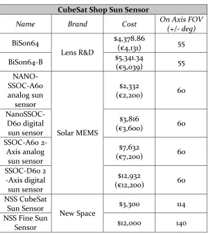
Table 2.10 – CubeSat Sun Sensor Options CubeSat Shop Sun Sensor

Name Brand Cost On Axis FOV

(+/- deg) BiSon64

Lens R&D

$4,378.86

(€4,131) 55

BiSon64-B $5,341.34

(€5,039) 55 NANO-SSOC-A60 analog sun sensor Solar MEMS $2,332

(€2,200) 60

NanoSSOC-D60 digital sun sensor

$3,816

(€3,600) 60 SSOC-A60

2-Axis analog sun sensor

$7,632

(€7,200) 60 SSOC-D60 2

-Axis digital sun sensor

$12,932

(€12,200) 60 NSS CubeSat

Sun Sensor

New Space

$3,300 114

NSS Fine Sun

Sensor $12,000 140

Table 2.11 – Sample CubeSat Horizon Sensors CubeSat Shop Infrared Horizon Sensors

Central Wavelength

(10e-6 m)

Height (mm) Diameter _(mm)

Infrared Band-Pass Filter 18 Type

HEAD $32,939.50

(€31,075) 15.1

1.5 18

Infrared Band-Pass Filter 18 Type

1.5

25 Infrared

Band-Pass Filter 18 Type

2 Infrared

Band-Pass Filter 18 Type

(45)

31

This factor has been incorporated into a new “On Board Computer” design driver for the Command and Data Handling Subsystem.

From these explorations and implications, the simplified map of the ADC design drivers is shown in Figure 2.8 below. An additional eight drivers were incorporated into the following figure as they impact the ADC subsystem drivers after combinations and simplifications. The “CubeSat Size” driver is a part of the Propulsion Subsystem and has already been discussed in Section 2.1. “On Board Computer” is a part of the Command and Data Handling (CDH) subsystem and will be discussed in the next section. “Center of Mass Offset,” and “Solar Array Area” are a part of the Mechanical subsystem and will be discussed in Section 2.6. “Layout” and “Temperature Range” are in Section 2.7 – the Thermal subsystem, and “Ground Station” and “Data Rate and Distance” are in the Telemetry Tracking and Command subsystem presented in Section 2.4.

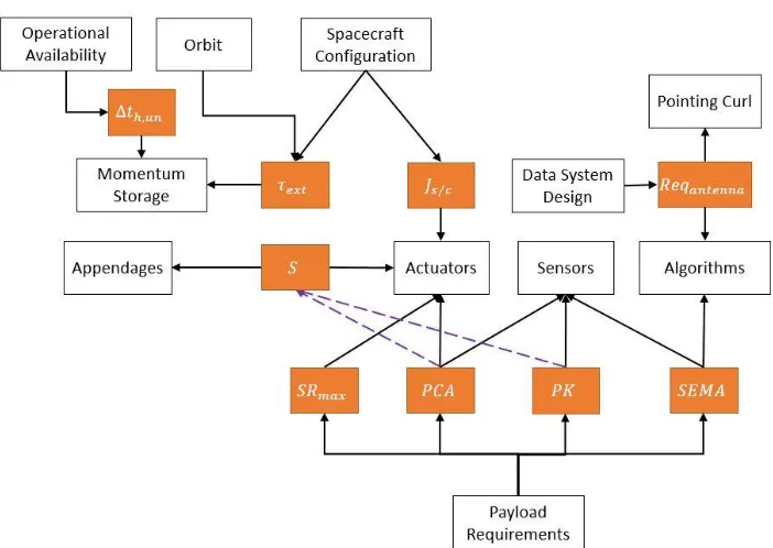
Figure 2.8 – Final Map of ADC Subsystem Drivers

2.3 Command and Data Handling (CDH) Design Drivers

(46)

32

Figure 2.9 – CDH Design Drivers

“Instrument Data Interface” involves the “hardware and software interfaces for commanding the payloads and reading the data impact the complexity of the C&DH.”[54] The “Processing Requirements” “define the speed of the processor, the dynamic memory (typically Random Access Memory or RAM), and the non-volatile memory (usually Programmable Read Only Memory, PROM, or Electrically Erasable Programmable Read Only Memory, EEPROM).” [54] The “Data Storage Volume” is the amount of memory needed to store the data collected by the payload. This is dictated by the amount of data generated by the payload and the ability of the spacecraft to downlink the collected data. “Timing Accuracy”, is the accuracy with which the spacecraft needs to keep time – by using an oscillator as a reference, the spacecraft is able to keep time by keeping track of the number of cycles performed since powering up the system. [54]

(47)

33

Figure 2.10 represents the simplifications made to the CDH subsystem map when considering a CubeSat architecture. The primary change was the combination of the “Payload” and “Payload Requirement” factors. After the initial simplification, the remaining factors and drivers were explored further do determine their importance in the system model and the creation of the mathematical model.

“Processing Requirements” “define the speed of the processor, the dynamic memory (typically Random Access Memory or RAM), and the non-volatile memory (usually Programmable Read Only Memory, PROM, or Electrically Erasable Programmable Read Only Memory, EEPROM).” [54] “Data Storage Volume” is the amount of memory needed to store the data collected by the payload. This is dictated by the amount of data generated by the payload and the ability of the spacecraft to downlink the collected data. “Instrument Data Interface” involves the “hardware and software interfaces for commanding the payloads and reading the data impact the complexity of the C&DH.”[54] “Timing Accuracy”, is the accuracy with which the spacecraft needs to keep time – by using an oscillator as a reference, the spacecraft is able to keep time by keeping track of the number of cycles performed since powering up the system. [54] Additionally, the “Algorithms” factor has also been incorporated into the new “On Board Computer” driver and the “Processor” factor itself is also included here.

An operations concept – also known as a mission concept or concept of operations – is a “broad statement of how the mission will work in practice.” [49] It is the plan by which the designed system will execute tasks to achieve the desired mission objectives. Typically for missions that need to relay information to the earth, there are four main elements in the operations concept: 1) data delivery, 2) tasking, scheduling, and control, 3) communications architecture, and 4) program timeline. [79] These aspects of the operations concept are developed by asking questions – like “How is imagery collected?” “Which forested areas are receiving attention this month?” and “What is the schedule for satellite replenishment?” – and by performing trade studies [79].

Oscillators on satellites are used as precision instruments essential to navigation systems, experiments, communications, and altimetry. [80] However, in CubeSats these oscillators are already incorporated.

(48)

34

“Algorithms,” and “Timing Accuracy” into the unified “On Board Computer” driver, two additional driver blocks were added to this system map: the “Power Consumption” and “Antenna” drivers. The “Power Consumption” driver is a part of the Power Subsystem and was added in place of the “Power” factor as the “On Board Computer” needs a certain amount of power in order to function. This new driver is addressed in Section 2.5 and the “Antenna” driver was addressed in the previous section on the Attitude Determination and Control Subsystem (Section 2.2).

Figure 2.11 – Final Map of the CDH Subsystem

2.4 Telemetry, Tracking and Command (TTC) Design Drivers

(49)

35

Figure 2.12 – TTC Design Drivers

“Data Rate & Distance” (𝐷𝑅𝐷) is rate at which data is communicated to the ground stations and the distance the data must go to reach the ground station. “Frequency” (𝑓), refers to the radio frequency on which the CubeSat is allowed to broadcast. “Ground Station Effective Isotropic Radiated Power” (EIRP), is a ground station parameter which is the combination of the transmitter power, antenna gain, and the ground station G/T ratio. [54] “Ground Station G/T ratio” (𝐺 𝑇⁄ ), is the antenna gain divided by the noise temperature of the receiver. [54] “Duty Cycle” (𝑐𝑦𝑐𝑑𝑢𝑡𝑦), is the fraction of one period in which a signal or system is active. [81] This subsystem did not immediately simplify based on CubeSat design requirements, in fact, as seen in Figure 2.13, a connection was added between “Ground Station G/T Ratio” and “Ground Station Effective Isotropic Radiated Power.”

Figure 2.13 – Simplified TTC Design Drivers

(50)

36

Since “Ground Station Effective Isotropic Radiated Power” and “Ground Station G/T Ratio” are things that are typically not selected independently for a CubeSat mission, they have been combined into one driver “Ground Station.” A sample of ground stations available for purchase are in Table 2.12. Each of these ground stations comes with: 1) and instrumentation rack containing the receiver, a PC with Local Ground Station Software, a rotator controller, and cavity filters to suppress UMTS interferences, 2) a steerable antenna system with lightning protection, 3) standard software with satellite tracking software pre-installed, and 4) the ability to operate remotely through the internet. Costs are presented in both Euros and United States Dollars (USDs) in the table below because the original price was in Euros and the prices were converted for consistency on April 15, 2017 when the exchange rate was 1.06 USDs to the Euro.

Table 2.12 – ISIS Full Ground Station Packages for Purchase [82] Ground Stations

Frequency Band Cost

S-Band $49,290

(€46,500)

VHF/UHF $43,990

(€41,500)

VHF/UHF/S-Band $59,890

(€56,500)

If the mission requires more continuous access to the spacecraft than a couple purchased ground stations can supply, then the other option is to purchase time on a previously established network. One of these networks is Spaceflight – through them you can purchase a radio (communications system) and data plans either per minute or per month with costs depending on the frequency used [83]. Other similar services are currently in development like BridgeSat, Leafspace, Atlas Ground, and Kongsberg Satellite Services [84–87], to name a few. Most of these companies do not publicly disclose their prices. But BridgeSat cost $1.95/minute for UHF versus $19.95/minute for S/X Band on the pay per minute plan and $3,000/month for UHF versus $50,000/month for S/X band on the pay per month plan.

The “Frequency” driver has also been incorporated into this section. “Frequency, 𝑓,” refers to the radio frequency on which the CubeSat is allowed to broadcast.

(51)

37

Power Subsystem and “Duty Cycle” was a driver for the TTC subsystem. In this work these two drivers have been combined into a single “Duty Cycle” driver.

“Data Rate and Distance” is the rate at which data is communicated to the ground stations and the distance the data must go to reach the ground station. As seen in Figure 2.13 there is also a “Data Rate” factor in addition to the “Data Rate and Distance” design driver. These two have been combined into a unified “Data Rate and Distance” driver. Though the data rate part of the “Data Rate and Distance” will be determined by the antenna specifications, the distance aspect is dependent on the network of ground stations and the orbit of the spacecraft. This will be explored further in the generation of the mathematical model in Chapter 3.

The quantity and type of battery selected will determine how much energy the system is able to store. A battery pack is comprised of individual cells connected in series and parallel. The number of cells required is determined by the bus voltage requirements, power consumed by the system, and the length of time the system will not be generating power. [88] It is important that the batteries of the spacecraft are able to store enough energy for the system to remain operational during eclipse periods. The following table include some details of batteries considered for use in the CubeSats generated by this study.

Table 2.13 – A sample of batteries found on CubeSatShop [89–91] Batteries

Name Brand

Power System Included Max Voltage (V) Watt Hours (Wh) BP4 2P-2S GomSpace

N 8.4 38.5

BP4 1P-4S N 16.8 38.5

BPX 2S-4P N 8.4 77

BPX 4S-2P N 16.8 77

BPX 8S-1P N 33.6 77

BM 1 2S2P Pumpkin N 8.25 40

EPS 1

EnduroSat

Y 4.2 10.4

EPS 1 Plus Y 4.2 20.8

EPS 2 Y 12.6 20.7

EPS 2 Plus Y 16.8 41.4

(52)

38

system is not in eclipse. The power consumed by the system will be the sum of the power consumed by the individual components.

Since the commercial off the shelf antennas have predetermined transmitters and receivers, “RF Transmit Power,” “Xmit Power,” and “Receiver Sensitivity” have all been combined into the “Antenna” driver.

Following the exploration of the design drivers and factors presented in Figure 2.13, the subsystem map of the Telemetry, Tracking and Command subsystem was reduced to Figure 2.14.

Figure 2.14 – Final Map of the TTC Subsystem

As seen in Figure 2.14 above, the number of drivers for the TTC subsystem has reduced from five design drivers to three. There are however two new design drivers – primarily associated with other subsystems – that have been included in this new system map: the “Antenna” and the “Solar Array Area” drivers. The “Antenna” driver is a part of the ADC subsystem and was discussed in Section 2.2. “Solar Array Area” is a part of the Mechanical Subsystem and will be discussed in Section 2.6.

2.5 Power Design Drivers

(53)

39

and maintenance of the satellite, the payload is the reason for the mission, and therefore takes precedence when designing the power subsystem. However, there are other drivers and factors that have been isolated from Figure 2.1 and are presented in Figure 2.15 below.

Figure 2.15 – Power Design Drivers