Perturbing and Protecting a Traceable Block Cipher
Julien Bringer, Herv´e Chabanne, Emmanuelle Dottax Sagem D´efense S´ecurit´e
Abstract
At the Asiacrypt 2003 conference Billet and Gilbert introduce a block cipher, which, to quote them, has the following paradoxical trace-ability properties: it is computationally easy to derive many equivalent distinct descriptions of the same instance of the block cipher; but it is computationally difficult, given one or even up tokof them, to recover the so-called meta-key from which they were derived, or to find any additional equivalent description, or more generally to forge any new untraceable description of the same instance of the block cipher.
Their construction relies on the Isomorphism of Polynomials (IP) problem. We here show how to strengthen this construction against algebraic attacks by concealing the underlying IP problems. Our mod-ification is such that our description of the block cipher now does not give the expected results all the time and parallel executions are used to obtain the correct value.
Keywords. Traitor tracing, Isomorphism of Polynomials (IP) prob-lem, perturbation.
1
Introduction
Traitor tracing was first introduced by B. Chor, A. Fiat and M. Naor [4]. This concept helps to fight against illegal distribution of cryptographic keys. Namely, in a system, each legitimate user comes with some keys. We sup-pose that a hacker can somehow have access to them, maybe because some legitimate users are traitors. These keys can then be duplicated, or new keys can be created by a pirate, computed from legitimate ones. Traitor tracing enables an authority to identify one or all of the users in possession of the keys at the origin of the pirated ones.
Today, many traitor tracing schemes are based on some key distribution and management techniques; the distribution of the keys is dependent on some combinatorial construction. A novelty comes in 1999 with D. Boneh and M. Franklin [3] (see also [10]) where public key cryptosystems are con-sidered.
At the Asiacrypt 2003 conference, Billet and Gilbert [2] propose a traitor tracing scheme taking place at a different level as the block cipher which al-lows the decryption of the signal, also permits the traitor tracing functional-ity. To this aim, a block cipher which have many descriptions is introduced. All descriptions give – of course – the same result. Their idea relies on the Isomorphism of Polynomials (IP) trapdoor [12], based on algebraic problems for multivariate polynomials over finite fields. It was supposed that from one or many descriptions of this block cipher it is not possible to create new ones both allowing to decrypt the broadcasted signal and preventing the author-ity to trace back pirates. However, recently, Faug`ere and Perret [9] have presented a new algorithm for solving IP-like instances and have achieved to solve a challenge proposed in [2].
Following the internal modifications of the Matsumoto-Imai cryptosys-tem from Ding [6], we add perturbations to Billet and Gilbert’s traceable block cipher. Doing so, we want to protect the trapdoors from direct alge-braic attacks (as for instance the recent algorithms of [7] and [9]), i.e. we want to alter the formal description of each round which forms the block cipher. However, here, we must still keep the traceable property with regard to the original block cipher. To manage this constraint, the pertubations are chosen in a particular way and we run in parallel, for each round, multiple descriptions of this round. None of them always gives the right result but we can show that a majority of these descriptions actually does, leading us to the expected value.
2
A traceable block cipher
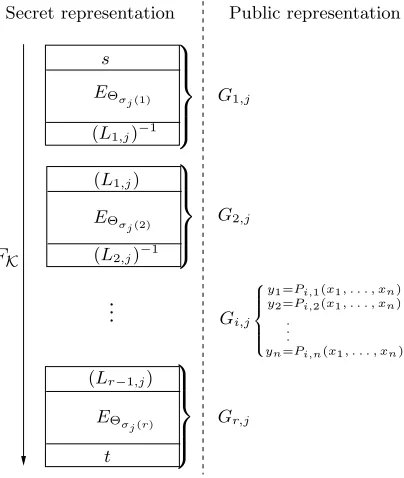
The traceable block cipher of Billet and Gilbert is made of a succession of rounds. Each round is given by a system of equations in a finite field F. The authority possesses a meta-key which allows it to compute the secret representations of the block cipher. The public representations consist of the suitable systems of polynomialsGi,j.
The left part of Figure 1 illustrates the secret authority description. Each round is made of a non-linear part preceded and followed by a linear transformation.
The invertible linear transformations Li,j depend on user j, the same
is true for the order in which non-linear parts occur in the block cipher. We call σj this permutation of the rounds. Thus, for user j, the system
of polynomials, giving his public representation of the rounds, is uniquely determined by the linear parts of the round Li,j and σj. It is computed
from the secret representation by the authority and lies in the right part of Figure 1. For userj, we denote them byG1,j, . . . , Gr,j.
PSfrag replacements 8 > > > > < > > > > :
y1=Pi,1(x1, . . . , xn)
y2=Pi,2(x1, . . . , xn)
. . .
yn=Pi,n(x1, . . . , xn)
.. .
Secret representation Public representation
FK
s
t g
FKj
EΘ
σj(1)
EΘ
σj(2)
EΘ
σj(r)
(L1,j)−1
(L2,j)−1
(L1,j)
(Lr
−1,j)
G1,j
G2,j
Gr,j Gi,j
^
M1◦G1,j M2◦G2,j◦M−1
1 Mi◦Gi,j◦M−1
i−1
^
Gr,j◦M−1
r−1
Modified representation
Here,
• r is the number of rounds,
• nstands for the number of variables,
• s, tand the Li,j are linear,
• theEΘσj(i) are non-linear,
• the polynomials Pi,1, . . . , Pi,n are homogeneous of degree d.
Remark 1 The linear transformations s and t are shared by all the users of the system.
What made this block cipher traceable is the property thatEΘi1◦EΘi2 =
EΘi2 ◦EΘi1, i.e. the non-linear parts commute, always leading to the same
function FK = t◦EΘσj(r) ◦ · · · ◦EΘσj(1) ◦s independently of the order σj
in which the rounds are given. The permutation σj on the order of the
rounds is unique for each user and allows the authority to recover him. More precisely, to this aim of finding a user from his block cipher description, first, the authority computes in turn, for eachi∈ {1, . . . , r},
G1,j◦s−1◦EΘi
−1, (1)
guessing the right value i by testing the simplicity of the result, i.e. by estimating the degree and the number of monomials. Whenσj(1) has been
found, the authority continues its procedure withG2,j◦G1,j◦s−1◦EΘσj(1) −1◦
EΘi
−1, fori6=σ
j(1), trying to find backσj(2), and so on, until the
permu-tation σj is entirely recovered, see [2] for details.
3
Our protection in a nutshell
We write ˜0 for a polynomial which often vanishes and ˜P =P + ˜0. By the way, ˜S stands for a system S of equations where some substitutions are made, replacing some polynomialsP by ˜P.
Our idea is to simply replaceGi,j byGgi,j, for i= 1, . . . , r. This way, the
IP problem structure of each round are made less accessible to an attacker. The construction where only one description of a round is modified is mainly given for pedagogical purpose and as an introduction to Sect. 5.2. Actually, it conducts to wrong results.
In order to have a function which gives us always the correct result, we have to modify several instances of the block cipher. More precisely, we replace the system Gi,j by 4 concurrent systems Ggi,j where we can prove
that two of them lead to what is expected. A majority vote allows to decide which result we have to retain. Note that this protection of one round can be seen as a protection of one IP-like instance, and this way, it could be applied to some other cryptographic schemes based upon IP.
4
Parasitizing the system with
˜
0
-polynomials
Example 1 is not sufficient because it does not allow enough diversity to stay hidden from an attacker. In this section, we introduce new ˜0-polynomials to this aim. We proceed following two steps.
First, we introduce a well-known class of polynomials, theq0-polynomials.
With them, we are able to compute polynomials which vanish on a predeter-mined set of points. However, asq0-polynomials are univariate and strongly
related to vector spaces, next, we have to compose them with random mul-tivariate polynomials.
4.1 Linearized polynomials [11]
Definition 1 For q0 a power of 2 such that q0 | q, a q0-polynomial over
F = GF(q) is a polynomial of the form L(X) = Pe
i=0aiXq0
i
, with e∈ N
and(a0, . . . , ae)∈Fe+1.
Note that aq0-polynomialL of degreeqe0 has at most e+ 1 terms and a
great number of roots in its splitting field. Indeed, ifa06= 0, we see that L
has only simple roots, so it hasqe
0 zeroes inF.
Example 2 LetTr :x7→P15i=0x2i
be the trace ofGF(216)overGF(2)and
α ∈ GF(216), then L = T r(α.X) is a 2-polynomial with 16 terms and 215 roots over GF(216).
Proposition 1 The set of a q0-polynomial roots is a linear subspace of its splitting field, i.e. L(X) = Pei=0aiXq0
i
subspace and some κ ≥ 1. In fact, for a q0-polynomial with simple roots,
κ= 1.
To count the number ofq0-polynomials withq0eroots of order 1, it suffices
to count the number ofGF(q0)-subspaces ofGF(q) of dimension e:
Corollary 1 For q = qm
0 , the number of q0-polynomials with qe0 roots of order 1 is equal to:
G(q0, m, e) =
(q0m−1)· · ·(qm−e0 +1−1) (qe
0−1)· · ·(q0−1)
.
Due to the finite field structure, it is clear that a q0-polynomial has
at most 2m−1 roots, so, if we want to construct ˜0-polynomials with more roots, we need to multiply severalq0-polynomials together. But, there would
be some intersection among the roots of different polynomials. Hence, to increase the number of roots more efficiently, we can combine some affine
q0-polynomials which are the relevant construction of q0-polynomials with
an affine set of roots.
Definition 2 For q0 a power of 2 such that q0 | q, an affine q0-polynomial overF=GF(q) is a polynomial of the formA(X) =L(X)−α whereα∈F
andL is a q0-polynomial.
4.2 Multivariate lifting
In order to tranform a q0-polynomial into a multivariate polynomial, we
compose it naturally with a multivariate polynomial.
Let Q be an affine q0-polynomial over GF(q0m) which equals zero over
the subspace U of dimension e, we construct a multivariate version of Q
by choosing a multivariate polynomialf ∈GF(qm0 )[X1, . . . , Xnf] and
com-puting Qf =Q(f(X1, . . . , Xnf)). In our context, two conditions have to be
considered :
1. the resulting polynomial must have at least the same proportion 2m1−e
of roots asQ,
2. Qf should not have a large number of terms.
Hence, we restrict the choice for f so as to respect the previous condi-tions. In practice, we take a random f with a small number of terms and we check if at least 1/2m−e points of GF(qm
0 )nf have an image following f
Example 3 IfQ= TrGF(24)/GF(2)(X), Qhas 8roots inGF(24). Then the
polynomial f(X1, X2) =X1+X1.X2 of GF(24)[X1, X2] gives a polynomial
Qf with at least 32 roots in GF(24)2.
Eventually, this method allows to obtain a multivariate polynomial and also to randomize the construction by breaking its linear structure.
5
Some practical considerations
In Sect. 5 of [2], the authors provide two examples of a system for 106 users.
In the first one, the base field isGF(216) and there are 5 variables. The block cipher has 32 rounds and each equation is homogeneous of degree 4, hence each round has at most 350 monomials, and there is at most 11200 monomials for the whole system. We will refer to this example as the Case 1.
In the second one, which we call Case 2, the base field is GF(29), there
are 19 variables, the block cipher has 33 rounds and each equation is homo-geneous of degree 3. So each round and the system have, respectively, at most 25270 and 833910 monomials.
5.1 Protecting one round
In this section, we introduce a modified system leading to the correct result more than half time. In particular, we explain the interferences of our parasitic ˜0 with the original public user representation; we show how we can choose some component H of ˜0 to prevent an attacker to retrieve the original system.
Let ˜0 =L(f(X1, . . . , Xnf))H(X1, . . . , Xn) where
• Lis a 2-polynomial with 2m−1 roots,
• f is a random polynomial of degree df in 2 ≤ nf ≤ n variables and
tf ≥2 terms such that 1/2 of its values are roots ofL,
• H is a random polynomial inn variables overF withtterms.
Proposition 2 The polynomial ˜0 has aboutN1(m, t, tf) terms and at least
1/2 of roots where
We add a parasitic ˜0 to every equation of the round, taking the same 2-polynomialLfor all equations of a given round but with different random polynomials H. This method allows the construction of a round function
g
Gi,j that gives the correct result with a probability greater than 1/2.
We introduce the polynomialHto generate enough monomials of degree
dto avoid the capability of recovering P, a homogeneous multivariate poly-nomial of degreed, from the knowledge ofP+ ˜0. In fact, starting fromP+ ˜0, one can immediately compute the polynomial ˜0 without its monomials of degree d, then knowing the form (i.e. designed as above) of ˜0, one can try the two following ideas:
1. Guess the unknown monomials and their coefficients among all of the different possibilities, in order to obtain a polynomial with the same specific structure as ˜0. There are Mn,d = n+d−d 1 monomials of
de-gree d in n variables, so even if one guesses the number k of missing monomials, there would be Mn,d
k
qk cases.
2. Analyse the terms ofP + ˜0 to guess the missing monomials, then, by deducing the generic form of H, try to find the missing coefficients by solving an overdefined system of equations, at least quadratic, in
t+lvariables over F(wherel is the number of variables coming from
the unknown 2-polynomial of ˜0 and from f). This kind of problem has been extensively studied these last years (see [5], [8] for example), and in general, one can not provide attacks in less thanq(t+l)/2, so we
should considertsuch that qt ≥2160.
The choice of f and H is made in the following way: we choose f with at least one term of degree 1 inX1 and ifI is the set of L(X1) exponents,
then we draw a polynomialH as
H(X1, . . . , Xn) =
X
i∈I∩{1,...,2m−1}
hi(X1, . . . , Xn)X12
m−i.d f,
where thehi ∈F[X1, . . . , Xn] are homogeneous of degreed−1. For each i,
letti be the number of terms of hi, then H has nearlyt=Piti terms and
the product L(f(X1, . . . , Xnf))H(X1, . . . , Xn) has at least t monomials of
degreed. Hence, the number of monomialskwhich are masking the original polynomialP is greater thant, so a choice oft, such thatqt ≥2160 to avoid
the second strategy above, allows also to thwart the first idea.
Furthermore, the number of choices forf andH is very large and so the amount of ways to interfere an equation is large enough.
• Case 1: We chooseL, f, H such thattf = 2 and t= 10, as described
above. This implies N(16,10,2) = 320 terms more for each equation, and thus 1600 terms more for one round Ggi,j. This represents nearly
6 times the size of the original round.
• Case 2: Fortf = 3 andt= 18 such thatqt ≥2160, we haveN(9,18,3) =
486 more terms for each equation. The resultingGgi,jhas hence around
1,4 times the size ofGi,j.
Remark 2 Roughly counting, there are more than Λ = G(2, m, m−1)× df
tf−1
×2mt+tf different ways to interfere an equation with such polynomials
˜0. In case 1, Λ≥2208, and in case 2, Λ≥2189.
5.2 Getting the correct value
For a given roundGi,j, we use four parallel modified descriptions Ggi,j with
correlated ˜0-polynomials to recover the expected result.
To achieve this goal, we partitionFand construct ˜0-polynomials
accord-ingly. As shown in Sect. 5.1, it is possible to cover more than half of F.
So, we partitionF twice into two sets of same size F=E1∪E1 =E2∪E2
and we construct ˜01, ˜01, ˜02 and ˜02 such that the polynomial ˜0κ (resp. ˜0κ)
vanishes over Eκ (resp. overEκ), κ= 1 or 2.
With this construction, for any input value, there is always two ˜0-polynomials which vanish and so at least two descriptions Ggi,j which give
the expected result. Furthermore, as the constuction of an ˜0-polynomial is partially random (see Sect. 5.1), the non-zero values of the two other ˜0-polynomials look like random ones. Hence, with an overwhelming proba-bility, the two other descriptions take 2 different results and so we can easily decide which value is correct according to a majority decision.
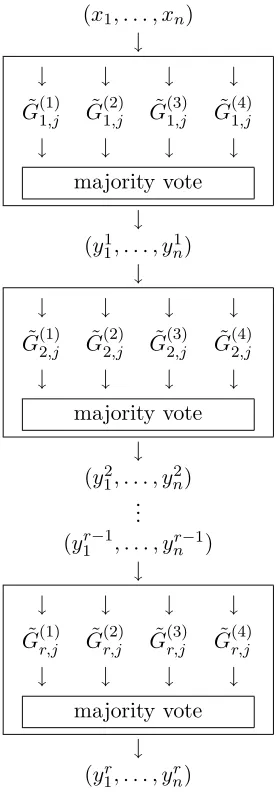
5.3 The final construction
Our new description of the entire public representation consists thus in mod-ifying each round independently as described in Sect. 5.2. We obtain four parallel systems, with a majority vote at each level to decide which value has to be sent to the next round. See Fig. 2 for the resulting description.
Then, the size of this description according to the two practical examples of [2] is:
(x1, . . . , xn) ↓
↓ ↓ ↓ ↓
˜
G1(1),j G˜(2)1,j G˜(3)1,j G˜(4)1,j
↓ ↓ ↓ ↓
majority vote
↓
(y1
1, . . . , yn1) ↓
↓ ↓ ↓ ↓
˜
G2(1),j G˜(2)2,j G˜(3)2,j G˜(4)2,j
↓ ↓ ↓ ↓
majority vote
↓
(y12, . . . , yn2) .. . (yr−1 1, . . . , yr−1
n ) ↓
↓ ↓ ↓ ↓
˜
G(1)r,j G˜(2)r,j G˜(3)r,j G˜(4)r,j
↓ ↓ ↓ ↓
majority vote
↓
(yr1, . . . , ynr)
Figure 2: New public representation
Thus, the final function (with 4 parallel systems of 32 rounds) contains around 22 times more terms than the original description.
5.4 Tracing procedure
Following [1], the authority can trace back pirates by looking at correlations between differential characteristics of the input and differential characteris-tics of the output. Thus, such a procedure relies only on the evaluation of rounds at given input contrary to the procedure described in [2] which is based on polynomials compositions.
This procedure, via evaluations, is still compatible with our new descrip-tion and can be used by the authority to trace back the traitors.
Acknowledgments. The authors thank gratefully St´ephanie Alt and Rey-nald Lercier for their comments on the tracing procedure.
References
[1] St´ephanie Alt and Reynald Lercier, private communication.
[2] Olivier Billet and Henri Gilbert,A Traceable Block Cipher, Advances in Cryptology – ASIACRYPT 2003 (C.S. Laih, Ed.), vol. 2894, 2003, pp. 331–346.
[3] Dan Boneh, and Mathew Franklin,An efficient public key traitor tracing scheme, Advances in Cryptology – CRYPTO’99 (Michael J. Wiener, Ed.), vol. 1666, 1999, pp. 338–353.
[4] Benny Chor, Amos Fiat, and Moni Naor, Tracing Traitors, Advances in Cryptology – CRYPTO’94 (Yvo Desmedt, Ed.), vol. 839, 1994, pp. 257–270.
[5] Nicolas Courtois, A. Klimov, Jacques Patarin, and Adi Shamir, Effi-cient Algorithms for Solving Overdefined Systems of Multivariate Polyno-mial Equations, Advances in Cryptology – EUROCRYPT 2000, vol. 1807, 2000, p. 392 ff.
[6] Jintai Ding, A New Variant of the Matsumoto-Imai Cryptosystem through Perturbation, Public Key Cryptography, 2004, pp. 305–318.
[8] Jean-Charles Faug`ere and Antoine Joux,Algebraic cryptanalysis of Hid-den Field Equation (HFE) cryptosystems using Gr¨obner bases, Advances in Cryptology – CRYPTO’03 (Dan Boneh, Ed.), vol. 2729, 2003, pp. 44-60.
[9] Jean-Charles Faug`ere and Ludovic Perret, private communication, February 2006.
[10] Aggelos Kiayias and Moti Yung,Traitor Tracing with Constant Trans-mission Rate, Advances in Cryptology – EUROCRYPT 2002 (Lars Knud-sen, Ed.), vol. 2332, 2002, pp 450–465.
[11] Rudolf Lidl and Harald Niederreiter,Intoduction to finite fiels and their applications, Cambridge University Press, 1986.