Tolerance of Pattern Storage Network for Storage and
Recalling of Compressed Image using SOM
M.P.Singh,
PhD Dr.B.R.Ambedkar UniversityKhandari Campus Agra, UP.
Rinku Sharma Dixit
Manav Rachna College of Engineering Aravalli Hills, Suraj-Kund Badkal Road, Fbd.,
Haryana
ABSTRACT
In this paper we are studying the tolerance of Hopfield neural network for storage and recalling of fingerprint images. The feature extraction of these images is performed with FFT, DWT and SOM. These feature vectors are stored as associative memory in Hopfield Neural Network with Hebbian learning and Pseudoinverse learning rules. The objective of this study is to determine the optimal weight matrix for efficient recalling of the memorized pattern for the presented noisy or distorted and incomplete prototype patterns from the Hopfield network. This study also explores the tolerance in Hopfield neural network for reducing the effect of false minimas in the recalling process. Besides this the capabilities of learning rules for pattern storage is also analyzed. This study also exhibits the analysis as pattern storage networks for feature vectors obtained from SOM with FFT and DWT
General Terms
Pattern Recognition, Image Analysis.
Keywords
Pattern Storage Network, Hopfield Neural Network, Associative Memory, SOM, Unsupervised Learning, Fast Fourier Transform, Discrete Wavelet Transform
1.
INTRODUCTION
Hopfield Network is probably the best known example of a Recurrent neural network working as associative memory [1, 2] for pattern storage and recalling of any type of graphical image patterns. These pattern storage networks with their energy surfaces behave similar to the associative memory architectures of the brain where the complete information can be recalled given only partial knowledge of the information content [3]. The dynamical behavior of the neuron states strongly depends on the synaptic strength between neurons and the used state updating scheme [4]. The specification of the synaptic weights is conventionally referred to as learning. Initially Hopfield used Hebbian learning to determine the network weights and since then a number of learning rules have been suggested to improve its performance [5, 6]. The Hebbian rule has associated with it the advantages of being local and incremental. This means that the update of a particular connection depends on the information available on either side of the connection and also patterns can be incrementally added to the network. This learning rule exhibits the following limitations:
The maximum capacity with binary input, as suggested by Hopfield, is limited to just 0.15N, if small errors in recalling are allowed. This was later revised to 0.138N (Amit, Gutfreund, Sompolinsky) using replica method [7]. While with bipolar
patterns the capacity is
N
N
2
log
2
, where N is the numberof neurons in the network [2].
The recall efficiency of the network deteriorates as the number of patterns stored in the network increases [8, 9].
The network’s ability to correct noisy patterns is also extremely limited and deteriorates with packing density of the network. New patterns could hardly be associated to the stored patterns.
Since Hebbian rule had the above mentioned limitations, other learning rules were considered to improve upon the learning behavior of the Hopfield Network. Pseudoinverse Rule is one of them. The standard Pseudoinverse rule is known to be better than the Hebbian rule in terms of the capacity, recall efficiency and pattern correction [2, 10]. The network capacity is of the order of L/N (where L represents the number of patterns in the network and N the number of neurons) and the retrieval efficiency falls sharply as the capacity approaches 0.5N [11, 12]. But Pseudoinverse rule is neither local nor incremental as compared to the Hebbian rule. These problems can be solved by modifying the rule in such a way that some characteristics of Hebbian learning are also incorporated such that locality and incrementality is ensured. Therefore the weight matrix is first calculated using Hebbian rule and then the Pseudoinverse of the weight matrix is calculated. This method may overcome the locality and incrementality problems associated with the Pseudoinverse rule. This exploration of the learning rule is implemented in the proposed study for the performance analysis of Hopfield neural network to ensure efficient pattern recalling. Pattern recalling for the memorized patterns is considered effectively if the pattern information is encoded sufficiently and efficiently. To accomplish the efficient pattern information the features from the input stimuli should be extracted firmly. There are various methods in literature that have been proposed for the feature extraction [13, 14, 15] to consider the task of associative memory phenomenon in Hopfield neural network architecture. In this context the methods like Fast Fourier Transform, Discrete Wavelet Transform and Self Organizing Maps have been identified as good ways for forming the pattern vectors to encode them into the pattern storage network as bidirectional autoassociative memory. Frequency domain filtering i.e. FFT and Space domain filtering i.e. DWT have proved to explore different aspects of the pattern spaces [13, 14, 16].
capability forms the basis of SOM functionality. The information is organized spatially and similar concepts are mapped to adjacent areas of the network. SOMs can thus be effectively used for clustering purposes. Apart from clustering, SOMs can also be used for dimensionality reduction. SOMs provide low dimensional representation of high-dimensional data akin to multidimensional scaling. SOMs transform an incoming pattern of arbitrary dimension into one or two-dimensional discrete map adaptively in a topologically ordered fashion. These maps learn to recognize groups of similar input vectors in such a way that neurons physically near each other in the neuron layer respond to similar input vectors. They provide a quantization of the image samples into a topological space where inputs that are nearby in the original space are also nearby in the output space, thereby providing dimensionality reduction and invariance to minor changes in the image sample. Pattern storage for continuum features as the input data can be characterized with the self organizing map and the Hopfield energy function analysis [20]. Map determines the feature mapping for the patterns with the continuum features. Iterations of the competitive learning between the input and the feedback output layer reduce the neighbouring region in the processing elements of feedback layer. On each iteration of this learning the used activation dynamics of the feedback layer leads the network towards the stable state. The feedback layer, which behaves as the Hopfield neural network, at the equilibrium stable state reflects the stored pattern at the minimum energy state. It reflects that we may explore the possibilities of mapping of the features from the pattern space to the feature space and simultaneously encode the presented patterns. The pattern vectors that consist with common features correspond to the same stable state of the pattern storage network.
In the proposed work we are studying and analyzing the tolerance of pattern storage networks of Hopfield type neural network for storage and recall for fingerprint images. The images obtained as scanned samples are first preprocessed and then filtered using FFT and DWT methods and then stored in the Hopfield Network. The storage capacity and recall efficiency of the Hopfield Network with the two categories of memorized images, when it is trained with Hebbian rule and with Pseudoinverse rule, will be tested. The next set of experiments is conducted to test the efficiency of the Hopfield Neural network for pattern recalling of the memorized images(filtered with either FFT or DWT) when the feature vectors are obtained with the Self Organizing maps. This will test the mapping of Self Organizing Maps with Hopfield Network. The pattern storage in the Hopfield network is effected through Hebbian and Pseudoinverse rules. The storage capacity and recall efficiency of such SOM-Hopfield network is also tested and analyzed. The results of the simulations are compared with each other. The simulation results show marginal enhancement in storage capacity and recall efficiency of the Hopfield neural network for the memorized and noisy feature vectors obtained from DWT filtering as compared to those obtained from FFT filtering with both Hebbian and Pseudoinverse learning rules. The next simulation i.e. SOM to Hopfield mapping shows drastic change in the performance. The network with FFT feature vectors almost collapses, with storage capacity reducing drastically with both Hebbian and Pseudoinverse rules. The recall efficiency with noisy patterns is also extremely limited. On the other hand with DWT feature vectors the storage capacity and recall efficiency with noisy patterns is substantially enhanced with both learning rules.
The paper is organized in following sections. Section 2 describes the FFT and DWT as the methods for the feature extraction to
create feature vectors for the input patterns. In section 3 the pattern storage network i.e. Hopfield Network and the two learning rules i.e Hebbian and Pseudoinverse used for storing the patterns are described. The next section describes the Self Organizing Maps. Section 5 depicts the simulation design and results. Observations, discussions of the obtained results and the future scope are specified in the last section followed by references in the last.
2.
FEATURE EXTRACTION
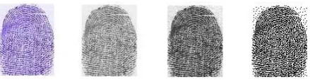
The feature extraction algorithms extract unique information from the images [13]. The pattern set used for the current study and analysis are scanned fingerprint images of multiple individuals. The images are not of perfect quality and thus require enhancement methods to reveal the fine details of the images which may remain uncovered due to insufficient ink or imperfect impressions. Hence images are preprocessed before converting them to suitable patterns for further processing. The images are first scanned as RGB images and then converted to Grayscale to retain the fine details in the images. After that the images are enhanced and made sharper using histogram equalization techniques. The resultant image is characterized by a histogram which is evenly spread as compared to a single peak in the original image depicting that the colors have been evenly spread to cover the entire 256 gray level spectrum. The image is finally converted into a binary image by thresholding about this histogram peak. The figure (1) depicts the different steps for preprocessing task.
Figure 1: a) Original Image, b) Grayscale Image, c) Histogram equalized image, d) Binarized image
The efficiency of the adopted feature extraction method decides to a great extent the quality of the image for further processing. Therefore we are employing method of FFT and DWT for feature extraction to consider the pattern for storage.
2.1
Fast Fourier Transform
Images are mathematically represented as a function of spatial variable f(x,y). The values of variables x and y at a particular location represent the intensity of the image at that point. This is the called the Spatial Domain representation of the image. An alternative representation of the same image can be through the representation of its frequency, phase or other complex exponentials. This is referred to as the Frequency Domain representation. Transforms are the mathematical representation of the Frequency Domain of the images. Transforms may be used for image enhancement, feature extraction, compression etc. Fast Fourier Transform (FFT) is a form of Fourier Transform whose input and output are discrete samples. The FFT is usually defined for a discrete function f(x,y) that is nonzero only over the finite region
0
x
X
1
and0
y
Y
1
. The two-dimensional X-by-Y FFT and [image:2.595.309.529.388.446.2]1 1
2 / 2 / 0 0
0,1,...,
1
( , )
( , )
0,1,...,
1
X Y
j px X j qy Y
x y
p
X
F p q
f x y e
e
q
Y
(2.1.1) and
1 1
0,1,...,
1
1
2
/
2
/
( , )
( , )
0,1,...,
1
0 0
X Y
j
px X j
qy Y
x
X
f x y
F p q e
e
y
Y
XY p q
(2.1.2)
The values F(p,q) are the FFT coefficients of f(x,y).
[image:3.595.55.294.71.191.2]We apply FFT on our binarized images producing the FFT transform. The filtered transform is then subjected to Inverse Transform to produce the refined images. Figure (2) represents the modified image after the FFT filtering of the binarized image.
Figure 2: Binarized Image and the image obtained after FFT Filtering
2.2
Discrete Wavelet Transform
Frequency based analysis slowly and steadily paved way to scale-based analysis when it started to become clear that an approach measuring average fluctuations at different scales might prove less sensitive to noise. Since, wavelets are characterized by scale and position; they are useful in analyzing variations in signals and images, which are best characterized in terms of scale and position. A wavelet is a waveform of effectively limited duration that has an average value of zero. When compared to sine waves, which form the basis of Fourier analysis, we realize that sinusoids do not have a limited duration and they extend from minus to plus infinity. Sinusoids being smooth and predictable, wavelets tend to be irregular and asymmetric.
Fourier analysis consists of expressing the original image in terms of the sum of basis functions which are the sinusoids of different frequencies. Wavelet analysis, on the other hand, expresses the original image in terms of a sum of basis functions, which are the shifted and scaled versions of the original (or mother) wavelet [13]. DWT cannot be described by one single equation or transform pair. Instead each DWT is characterized by a transform function pair or set of parameters that define the pair. The various transforms are related by the fact that their expansion functions are small waves or the so-called wavelets of varying frequencies and limited durations. Transform functions also called the wavelets are obtained from a single prototype wavelet called mother wavelet by dilations and shifting as:
,
1
( )
a b
t
b
t
a
a
(2.2.1)
Where, a is the scaling parameter and b is the shifting parameter. The transform functions can be represented by three separable 2-D wavelets and one separable 2-2-D scaling function
( , )
( ) ( )
( , )
( ) ( )
( , )
( ) ( )
( , )
( ) ( )
H
V
D
x y
x
y
x y
x
y
x y
x
y
x y
x
y
(2.2.2)
Where,
( , ),
( , ),
( , )
H V D
x y
x y
x y
are called horizontal, vertical and diagonal wavelets respectively and
( , )
x y
is the scaling function. FWT is an iterative [image:3.595.312.466.535.588.2]computational approach to the DWT. The digitized binary images are subjected to DWT filtering and the corresponding component wavelets are obtained. Consequent to the filtering the refined and filtered images are obtained by Inverse DWT. The crisper image obtained after DWT Filtering is depicted in the figure 3.
Figure 3: Binarized Image and the image after DWT Filtering
The images obtained after FFT and DWT filtering were then converted to bipolar patterns, since Pattern Storage Networks normally work better with bipolar patterns. A bipolar image is one where each pixel has value either +1 or -1. Finally the image, scaled to dimension 30 x 30, is converted to bipolar pattern vectors.
The general form of the
l
th pattern vector is:
1,
2,
3,...,
T
l l l l lN
x
x
x
x
x
where N=1 to 900
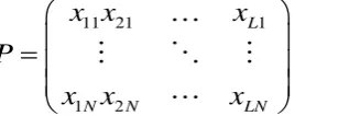
All the image pattern vectors are presented to the feedback network for storage in the form of a comprehensive matrix of order N x L as:
11 21 1
1 2
L
N N LN
x x
x
P
x x
x
(2.2.3)
Where L is the total number of images or patterns stored in the network and each pattern is a vector of order N x 1, where the value of N is 900.
3.
HOPFIELD NEURAL NETWORK
3.1
Pattern Storage
Hebbian Rule: The Hebbian Rule to store L patterns is given by the summation of correlation matrices for each pattern as:
1
1
*
for i
j
0 for i=j, 1 i
N
Lij li lj
l
W
x
x
N
(3.1.1)
where,
N is the number of units/neurons in the network
l
x
for l = 1 to L are the patterns / images to be stored, where
each component of
x
l is bipolar.For storing L patterns there should be one stable state corresponding to each stored pattern. Thus the following activation dynamics equation must be satisfied to accomplish the storage. The units receive input from every other unit except for itself. The net input of a unit i at any time t is computed as:
( )
( )
i ij j
j i
s t
w s t
(3.1.2)
where
w
ij is the weight of the connection between unit i and jand
s
j is the state of unit j at time t [9, 21].Consider the initial weights
w
ij
0
prior to learning between processing units i and j where i, j = 1 to N. The change in weight to store the 1st pattern can be considered as:1 1
,
new old
ij ij i j
i j
w
w
x
x
(3.1.3)
And
old new
ij ij
w
w
(3.1.4)
Similarly for the Lth pattern
1
,
L L
ij ij Li Lj
i j
w
w
x
x
(3.1.5) This can be generalized as
1 ,
L L
ij li lj
l i j
W
x
x
(3.1.6) The weight matrix thus obtained is normalized over all N. Hence the normalized weight matrix is given by
1 ,
1
L Lij li lj
l i j
W
x
x
N
(3.1.7)
The same weight matrix can be computed from pattern vectors as below:
1
1
( )
L L
l l
l
W
x
x
N
(3.1.8)
Thus after the final learning for all patterns, the final weight matrix can be represented as:
1 2 1 2 1
2 1 2 3 2
1 2
0 x
x
. . . x
0 x
. . . x
. . . .
x
. . . . 0
N
N L
N N
x
x
x
x x
x
x
W
x x
x
(3.1.9)Pseudoinverse Rule: The next rule which is used to store the patterns in the hopfield neural network is Pseudoinverse Rule. The standard Pseudoinverse rule is known to be better than the Hebbian rule in terms of the capacity, recall efficiency and pattern correction [2, 10]. The network capacity is of the order of L/N and the retrieval efficiency falls sharply as the capacity approaches 0.5N [11, 12].
Considering the training set P of patterns which contain L patterns each of size N, the pseudoinverse weight matrix is given by
†
W
PP
(3.1.10)where P is the matrix whose rows are
x
n andP
† is its pseudoinverse [8, 9].But Pseudoinverse rule is neither local nor incremental as compared to the Hebbian rule. These problems can be solved by modifying the rule in such a way that some characteristics of Hebbian learning are also incorporated such that locality and incrementality is ensured. Hence the weight matrix is first calculated using Hebbian rule stated in equation (3.1.9) then the pseudoinverse of the weight matrix can be obtained as:
† † 1
(
) (
*(
) )
L L L L
pinv
W
W
W
W
(3.1.11)
where
†
(
W
L)
is the transpose of the weight matrix LW
† 1
(
L(
L) )
W
W
is the inverse of the product of L
W
and its transpose.3.2
Pattern Recall
Once the pattern set P has been stored in the Hopfield neural network using either the Hebbian or the Pseudoinverse rule, it is required that the performance of the network be tested for the memorized patterns, their noisy variants and also for incomplete pattern information. For this, the process of recalling is considered, whereby a test pattern, which can be the memorized pattern or its noisy form, is input into the network and the network is allowed to evolve through its activation dynamics. The output state of the network is then tested for resemblance with one of the expected stable states.
Consider a memorized pattern X and its noisy or distorted form
X
where
is the induced error in terms of the percentage (number) of bits distorted i.e. 20% (180) bits, 30% (270) bits, 40% (360) bits and 50% (450) bits. Let the state ofthe network corresponding to the stored th
l
pattern is:
1 2
( )
l l,
l,...,
lNN s
s s
s
This represents one of the stable states of the network for the
memorized th
l
pattern. For recalling the stored fingerprintimage, the prototype pattern X and its noisy form
X
are presented to the network. The activation dynamics of the network produces the output state for X andX
respectively as:1
( )
( )(
1)
N
l k l
i ij j
j
s
w s
t
(3.2.2)
1
(
)
(
)(
1)
N
l k l
i ij j
j
s
w s
t
(3.2.3)
The activation dynamics, in (3.2.2) for the memorized pattern X and in (3.2.3) for the distorted form of X, is executed for testing the recall efficiency with Hebbian learning using the weight matrix obtained in (3.1.9) and with Pseudoinverse learning using the weight matrix obtained in (3.1.12).
If
( )(
1)
( ); i=1:N
l l
i i
s
t
s t
(3.2.4)
And
(
)(
1)
( ); i=1:N
l l
i i
s
t
s t
(3.2.5)
It implies that the network settles in the same stable state that corresponds to the already stored pattern.
4.
SELF ORGANIZING MAPS
Self Organizing Maps are single layer feed forward neural networks where the output syntaxes are arranged in low dimensional i.e. 2D or 3D grid. The neurons are placed at the nodes of an n-dimensional lattice. Each input is connected to all output neurons. Attached to every neuron there is a weight vector with the same dimensionality as the input vectors. SOMs differ from competitive layers in the way that neighboring neurons in the self organizing map learn to recognize neighboring sections of the input space. Thus, self organizing maps learn both the distribution and the topology of the input vectors. The neurons are connected to adjacent neurons by a neighborhood relation, which dictates the topology and structure of the map. The basic algorithm of SOM can be described as: SOM Algorithm
SOM is trained iteratively. All weights are initially set to small random values.
Step 1: Competitive Process: For each input pattern, each neuron computes its value for a discriminant function. The neuron with the highest value is declared the winner.
Let x be the input pattern and let m denote its dimension
1,
2,...,
m
x
x x
x
The weight vector for each of the neurons in SOM also has dimension m. Hence for neuron j, the weight vector will be:
1
,
2,...,
j j j jm
w
w
w
w
For an input pattern
x
i computex
i
w
ij for each neuron and choose the smallest value thus obtained. Let i denote the index of the winning neuron.Step 2: Cooperative Process: The winning neuron determines the spatial location of a topological neighborhood of excited neurons. The neurons in the neighborhood may then cooperate. The importance of the neighborhood lies in the fact that weight adjustment is done only for the neurons that lie in the neighborhood of the winning neuron. Further the size of the neighborhood shrinks with time thus localizing the area of maximum activity.
Step 3: Synaptic Adaptation: Excited neuron and all the neurons in its activated neighborhood increase their values of the discriminant function in relation to the current input pattern by weight adjustment. The rule for weight update can be defined as:
(
1)
( )
( )(
( )) i
h ( )
ij ij i ij ji
w t
w t
t x
w t
t
where
x
i is the input pattern( )
t
is the learning rate( )
ji
h t
is the neighborhood function defining the region around the winner neuron
The adaptive process has the following two stages:
Self Organizing Phase: This is an iterative phase where topological ordering of weight vectors is done. The phase starts with learning close to 0.1 and decreases it gradually but keeps it above 0.01. The neighborhood centered on the winner initially includes almost all neurons but slowly shrinks to only a couple of neighboring neurons.
Convergence Phase: It is used for fine tuning the map. The number of iterations is approximately 500 times the number of neurons. The learning rate is maintained at a small value i.e. 0.01 and the neighborhood is further decreased to only one or zero neighbors.
It is well known that, the self-organizing maps can be used for the feature mapping [22]. The feature map can often be effectively used for the feature extraction from the input data for their recognition or, if the neural network is a regular two-dimensional array, to project and visualize high two-dimensional signal spaces on such a one or two dimensional display [23]. Thus, the self-organizing map is an effective tool for the visualization of the high dimensional data in reduced dimensions. It converts the non-linear statistical relationship between high dimensional data into simple geometric relationships of their image points on a low dimensional display, usually a regular two-dimensional grid of nodes. It is used to deal for the patterns which represent the continuity in the feature space. The features extracted from the SOM can be used as patterns for storing or encoding in the feedback neural network of Hopfield type. The associative memory feature of Hopfield neural network for pattern storage and their recalling can be accomplished to incorporate symmetric feedback synaptic interconnection between the processing units of the output layer in self organizing map. The processing units of the grid in SOM i.e. the feedback neural network architecture for the pattern storage are considered as bipolar units. Obviously it is quite interesting to incorporate feedback connections among the processing units of grid in SOM for pattern recognition [22, 24]. It follows the competitive learning in unsupervised mode with non-linear output function for units in the feedback layer as shown in the figure 7 [20].
connection strength represented with weight vector M. The processing elements of the input layers are connected to each of the processing element of the feedback layer with connection strength represented with weight vector W. The presented input pattern to the network is K-dimensional with continuum features, applied one at a time. The network trained to map the similarities in the set of input patterns and at any given time only few of the input may be turned on. That is, only the corresponding links are activated to accomplish the aim of capturing the features in the space of input pattern and the connections are like soft wiring dictated by the unsupervised learning mode in which the network is expected to work [25]. There are several ways of implementing the feature mapping process. In one of the method, output layer is organized into predefined receptive fields, and the unsupervised learning should perform the feature mapping by activating the appropriate connections [26-28].
Another method of implementing the feature mapping process is to use the architecture of a competitive learning network with on center off surround type of connections among units, but at each stage the weights are updated not only for the winning units, but also for the units in its neighborhood [7]. This neighborhood region may be progressively reduced during learning. Let us consider the set of input variables {xi} defined as the real vector
X
{ ,
x x x
1 2,
3,...,
x
k}
R
n. This input pattern vector is applied to the processing elements of the input layer. The processing elements of the input layer are connected with each element in the SOM grid. This grid contains the feedback layer region. We associate connection strength
1,
2,....,
T n
i i i in
W
w w
w
R
to every processingelement of the feedback layer. The initial value of
W
T is selected randomly. Now the input pattern vector X is applied on the processing units of the input layer. The linear output of these processing units feed the weighted input through feed forward connection to the SOM grid. The activation of thej
th processing unit of the feed back layer can be represented as:1
K
j ij i
i
y
w x
(4.1)
where, j =1 to N (Number of units in the feed back layer.)
A winning unit, say P, is selected among all the processing units of the feedback layer as:
y
max
(
y
)
j i p
for all j
T T
P j
W X
W X
Geometrically the above relationship means that the input vector X is closest to the weight vector
w
pamong allw
i i.e.1 1
(
)
(
)
K k
i Pi i ji
i i
x
w
x
w
for all j (4.2)
Hence, during learning the nodes those are topographically close up to certain geometric distance will activate each other to learn from the same input vector X and the weights associated with the winning unit P and its neighboring units r are updated as:
)]
(
)
(
)[
,
(
)
(
)
1
(
t
w
t
P
r
x
t
w
t
w
iP
iP
i
ij (4.3)For i =1 to K and j =1 to N, here
( , )
P r
is the neighborhood function and it can be represented as [29]:]
2
exp[
.
)
,
(
2 2
R
PR
rr
P
(4.4)Where
R
P refers to the position of theP
th unit in the grid,r
R
refers to the position of the neighboringr
th unit, is learning rate constant (0< <1) and the parameter define the width of the Gaussian function. The will gradually decrease to reduce the neighborhood region in successive iterations of the training process. Therefore, with this mechanism of competitive learning, the SOM is able to learn in unsupervised mode the feature mapping of the input pattern with continuum feature space.5.
SIMULATION DESIGN AND RESULTS
In this simulation design and implementation experiments to design the proposed Hopfield Neural Network will be considered with 900 processing units. This feedback neural network is trained for pattern storage with two learning rules i.e. Hebbian Rule and Pseudoinverse Rule. The patterns being considered for storage have been preprocessed and filtered through FFT and DWT separately. In these experiments we are analyzing the storage capacity and recall efficiency for the memorized patterns from this neural network with the two learning rules. The pattern storage can be described in algorithmic form as.
Pattern Storage Hopfield Hebbian Rule ()
{
initialize weight matrix of size N x N to zero;
do
{
multiply pattern l with its transpose;
add product matrix to weight matrix;
}
while l not equal to L
assign zero to the diagonal elements;
normalize weight matrix by dividing each element by N;
}
Pattern Storage Hopfield Pseudoinverse Rule ()
{
initialize weight matrix of size N x N to zero;
do
{
multiply pattern l with its transpose;
}
while l not equal to L
assign zero to the diagonal elements;
normalize weight matrix by dividing each element by N;
calculate the pseudoinverse of the weight matrix;
}
The pattern information of the training set is encoded in the terms of weights between interconnection of the neurons. The final parent weight matrix is thus created which contains the encoded pattern information of the memorized patterns.
Thereafter the process of recalling is initiated for prototype input patterns of already memorized patterns. The recall efficiency provides an indication of the storage capacity of the network. The network is also analyzed for noisy prototype input or incomplete patterns. The test prototype pattern is input to the Hopfield network and then its activation dynamics starts iteration. The network finally settles into one of the stable states. This stable state corresponds to one of the memorized pattern that the input prototype pattern best matches. This recall has the possibility of settling into false minima. The network’s efficiency with new patterns not memorized in the network is also checked that whether it is able to associate it to one of the memorized patterns during its convergence cycle or to some false minima or no recognition at all. The pattern recall can be described in algorithmic form as:
Pattern Recall Hopfield ()
{
read the parent weight matrix;
input the prototype input pattern;
initialize input pattern to the network;
do
{
do for each randomly selected unit n
{
compute the net input to n;
add the net input to the existing value of n;
compare n with threshold;
set activation of n to +1 if n greater than threshold else to - 1;
broadcast the value of n to all other units;
}
while (n not equal to N)
}
while (convergence not achieved or 200 iterations)
}
The resulting storage capacity of the Hopfield network with
Hebbian learning is
2
2 log
N
N
as the network with 900 neurons is able to perfectly store 150 patterns and thereafter stops recalling one or the other memorized pattern. The preprocessing in terms of FFT or DWT filtering of the patterns does not impact this capacity. On the other hand with Pseudoinverse learning the storage capacity is sufficientlyenhanced and even 400 memorized patterns are correctly recalled.
The results depicting the recall efficiency of the Hopfield Network for prototype noisy patterns filtered with FFT and DWT have been shown in Table 1. The graph in figure (4) diagrammatically depicts the analysis specified in Table 1.
The recall efficiency has been analyzed at various packing densities of the network i.e. 40, 70, 100, 130, 150, 180, 200 and 230 patterns. At all packing densities the prototype patterns were distorted by explicitly introducing noise upto percentages as 30%, 40% and 50% by modifying 270, 360 and 450 bits respectively. The results are clearly in favour of the modified form of Pseudoinverse rule. The Pseudoinverse rule performs best with DWT filtered patterns with the performance dropping marginally with FFT filtered patterns at all packing densities. The rule is seen performing well even at packing density of 200 and thereafter slowly starts degrading for high distortion levels in the prototype patterns. It is also observed that the occurrence of false minima is negligible at lower distortions but at 50% distortion the network depicts a tendency of settling into false minima for some of the patterns. The Hebbian rule similarly shows better recall efficiency with DWT filtered patterns than with FFT filtered patterns. The recall efficiency and performance of Hebbian rule starts degrading beyond the packing density of 100 patterns
Now, the next experiment is conducted for feature extraction with SOM and mapped into the Hopfield neural network. In this simulation the input images preprocessed with either FFT or DWT and compressed using SOM before storing them into the Pattern Storage Network. The training set of L patterns is fed through a sequential algorithm into the Self Organizing Map of dimension 10 x 10 and with hexagonal topology. The storage of input patterns into SOM can be described with the following algorithms.
Self Organizing Map Algorithm ()
{
randomly initialize all weights;
for each input vector x;
do
{
apply x to each neuron in the SOM grid;
each neuron computes its value of the discriminant function;
select the winner neuron such that it has the maximum value;
update winner by weight adjustment so that it becomes more like x;
adjust parameters like learning rate and neighbourhood function;
}
while (map converges or 200 iterations)
}
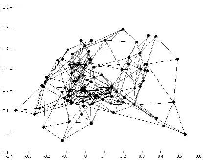
Figure 4: SOM grid created after input of patterns
The 100 feature vector of 900 x 1 input vectors of images are generated by SOM and these are converted into bipolar vectors. These pattern vectors are passed as input to the Pattern Storage Network. The pattern storage is done with hebbian and pseudoiverse rules as per the algorithms already stated. Recalling of the patterns involves presenting a prototype or noisy pattern for the already memorized patterns as input to the trained SOM. SOM in response will map it to the BMU (Best Matching Unit) in the grid map. The codeword corresponding to the BMU is then presented to the Hopfield network and the pattern recalled is the one that best matches the prototype input. The Hopfield network with memorized patterns encoded with hebbian and pseudoinverse will behave differently for the prototype input patterns and their noisy variants. The network is also analysed for noisy variants of the memorized patterns. Such patterns when presented to SOM, are mapped to the neuron with closest weight values termed the BMU. The codebook vector of the BMU is converted to feature vector and mapped to Hopfield Network. The Hopfield network starts iterating and settles into one of the stable states. This stable state corresponds to one of the memorized patterns or to false minima. The recall process for this SOM-Hopfield mapping can be depicted in the following algorithm as:
Pattern Recall Self Organizing Map-Hopfield Algorithm () {
read the trained SOM;
input the prototype input pattern;
apply the input to each neuron in the SOM grid;
select the BMU that best resembles the input vector;
select the codebook vector corresponding to the BMU;
create feature vector for the codebook vector;
read the parent weight matrix of Hopfield;
input the feature vector;
initialize feature vector to the network;
do
{
do for each randomly selected unit n
{
compute the net input to n;
add the net input to the existing value of n;
compare n with threshold;
set activation of n to +1 if n greater than threshold else to -1;
broadcast the value of n to all other units;
}
while (n not equal to N)
}
while (convergence not achieved or 200 iterations)
}
The results obtained for this experiment have been summarized in Table 2. Figure (6) shows a graph depicting a comparative analysis of the storage capacities of the Hopfield network in the two simulations discussed in this work It shows clearly that the Hopfield Network has uniform results when it trained with FFT and DWT filtered patterns using Hebbian and Pseudoinverse rules and also that the pseudoinverse rule outperforms in both cases. On the other hand the SOM-Hopfield (designated SH) mapped network shows contrasting results. The SOM-Hopfield network when trained with FFT filtered patterns shows poor results as compared to the Hopfield network. The storage capacity with hebbian rule is reduced to 70 (which in mathematical terms can be represented as
2 1
2 log 2
N N
)
while that with Pseudoinverse rule is reduced to 100. But on the other hand the same network when trained with DWT filtered patterns shows enhanced storage capacity with both the learning rules. With hebbian rule the capacity increases to 250 patterns which can be expressed in mathematical notation as 0.28N while with pseudoinverse rule the capabilities are further enhanced and even 600 i.e. beyond 0.5N memorized patterns are perfectly recalled.
0 50 100 150 200 250
30% 40% 50% 30% 40% 50% 30% 40% 50% 30% 40% 50% 30% 40% 50% 30% 40% 50% 30% 40% 50% 30% 40% 50%
40 patterns 70 patterns 100 patterns 130 patterns 150 patterns 180 patterns 200 patterns 230 patterns
P
a
tt
e
rn
c
orre
c
ti
on
a
nd
re
c
a
ll
e
ff
ic
ie
ncy
Total no of patterns at various distortion percentages Hopfield Network Pattern Correction and Recall Efficiency
[image:9.595.60.537.240.379.2]FFT Hebb's Rule FFT Pseudoinverse Rule DWT Hebb's Rule DWT Pseudoinverse Rule
Figure 5: Comparative Analysis of the Pattern Correction and Recall Efficiency of the Hopfield Network for the FFT and DWT Filtered Patterns
0 50 100 150 200 250 300 350 400 450
40 70 100 130 150 180 200 230 250 280 310 350 400
T
o
ta
l N
o
.
o
f
P
a
tt
e
rn
s
i
n
t
h
e
N
e
tw
o
rk
Pattern Storage Efficiency
Critical Storage Capacity
[image:9.595.75.533.392.547.2]Hopfield FFT Hebb's rule Hopfield DWT Hebb's Rule SH-FFT Hebbian SH-DWT Hebbian Hopfield FFT Pseudoinverse Rule Hopfield DWT Ps eudoinv ers e Rule SH-FFT Ps eudoinv ers e SH-DWT Ps eudoinv ers e
Figure 6: Comparative Analysis of the Critical Storage Capacity of the Hopfield Network
0 50 100 150 200 250 300 350 400 450
20 30 40 50 20 30 40 50 20 30 40 50 20 30 40 50 20 30 40 50 20 30 40 50 20 30 40 50 20 30 40 50 20 30 40 50 20 30 40 50 20 30 40 50 20 30 40 50 20 30 40 50
40 70 100 130 150 180 200 230 250 280 310 330 400
P
a
tt
e
rn
Co
rr
e
c
ti
o
n
a
n
d
Re
ca
ll
E
ff
ic
ie
n
cy
Total No of patterns in the network at various distortions percentages
SOM-Hopfield Pattern Correction and Recall Efficiency
FFT Hebbian
FFT Pseudoinverse
DWT Hebbian
DWT Pseudoinverse
Figure 7: Comparative Analysis of the Pattern Correction and Recall Efficiency of the Hopfield Network for the FFT and DWT Filtered Feature Vectors produced by SOM
Table 1: Pattern Recall Ability Of Hopfield Network With Prototype Noisy Patterns Filtered with FFT and DWT
Total No. of Patterns in the Network
Noise or % distortion in actual pattern
FFT Filtered Patterns DWT Filtered Patterns
Hebbian Pseudoinverse Hebbian Pseudoinverse
Pattern Association Pattern Association
Correct Recalling
False Minima
Correct Recalling
False Minima
Correct Recalling
False Minima
Correct Recalling
False Minima
70 patterns
30% 70 0 70 0 70 0 70 0
40% 70 0 70 0 70 0 70 0
50% 0 6 0 18 0 2 0 7
130 patterns
30% 54 0 130 0 80 0 130 0
40% 29 4 130 0 56 2 130 0
[image:9.595.95.504.594.769.2]180 patterns
30% 0 0 180 0 9 0 180 0
40% 0 0 36 24 0 0 47 21
50% 0 0 0 0 0 0 0 0
230 patterns
30% 0 0 128 0 0 0 147 0
40% 0 0 0 0 0 0 0 0
[image:10.595.93.495.201.757.2]50% 0 0 0 0 0 0 0 0
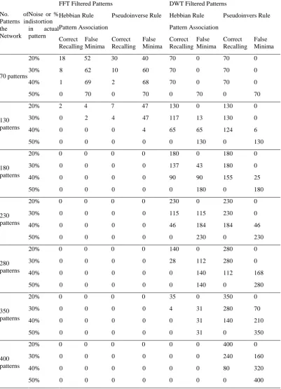
Table 2: Pattern Recall Ability of Hopfield Network Of The FFT and DWT Filtered Feature Vectors Produced by SOM
No. of
Patterns in the Network
Noise or % distortion in actual pattern
FFT Filtered Patterns DWT Filtered Patterns
Hebbian Rule Pseudoinverse Rule Hebbian Rule Pseudoinvers Rule
Pattern Association Pattern Association
Correct Recalling
False Minima
Correct Recalling
False Minima
Correct Recalling
False Minima
Correct Recalling
False Minima
70 patterns
20% 18 52 30 40 70 0 70 0
30% 8 62 10 60 70 0 70 0
40% 1 69 2 68 70 0 70 0
50% 0 70 0 70 0 70 0 70
130 patterns
20% 2 4 7 47 130 0 130 0
30% 0 2 4 47 117 13 130 0
40% 0 0 0 4 65 65 124 6
50% 0 0 0 0 0 130 0 130
180 patterns
20% 0 0 0 0 180 0 180 0
30% 0 0 0 0 137 43 180 0
40% 0 0 0 0 90 90 155 25
50% 0 0 0 0 0 180 0 180
230 patterns
20% 0 0 0 0 230 0 230 0
30% 0 0 0 0 115 115 230 0
40% 0 0 0 0 46 184 184 46
50% 0 0 0 0 0 230 0 230
280 patterns
20% 0 0 0 0 140 0 280 0
30% 0 0 0 0 28 112 280 0
40% 0 0 0 0 0 140 112 168
50% 0 0 0 0 0 140 0 280
350 patterns
20% 0 0 0 0 35 0 350 0
30% 0 0 0 0 4 31 280 70
40% 0 0 0 0 0 31 140 210
50% 0 0 0 0 0 31 0 350
400 patterns
20% 0 0 0 0 0 0 400 0
30% 0 0 0 0 0 0 240 160
40% 0 0 0 0 0 0 80 320
6.
CONCLUSIONS
Pattern Storage networks have been used to efficiently store and recall the prototype patterns. The learning method used traditionally has been Hebbian learning, which has with it a number of efficiency issues particularly related to the limited storage capacity and recall efficiency of the noisy prototypes. This can be taken care of by modifying the learning rule and also by adopting better methods of feature extraction. Experiments conducted in the current paper have tested both. The Pseudoinverse learning rule in this paper has been modified in such a way that it improves the storage and recall efficiency of the Hopfield network, a characteristic of the standard Pseudoiverse rule, and also incorporates some of the advantages of Hebbian rule such as locality and incremental learning. The feature extraction mechanisms chosen for this paper i.e. FFT, DWT and SOM have been implemented with Hebbian learning and with the modified Pseudoinverse learning and the results analyzed and compared. It has been analyzed through the simulation design that t he
efficiency of the Hopfield network can be enhanced by training it with modified Pseudoinverse rule instead of Hebbian rule. The Hopfield network performs better when the prototype patterns presented to it have been filtered through FFT and DWT and the feature vectors thus produced are stored into the network. The two methods have almost the same results but DWT slightly outperforms FFT. The efficiency of the Hopfield network can be further enhanced when the feature vectors produced by FFT and DWT are first compressed with SOM and the compressed feature spaces are input to the Hopfield network. Here the network receiving DWT filtered patterns performs well and improves both the storage capacity and recall efficiency but network receiving FFT filtered patterns performs poorly.
The following observations have been made during the implementation of the simulation design and analysis of the Hopfield neural network for pattern recalling of the memorized pattern vectors of the scanned images.
The capability of the Hopfield neural network in terms of the pattern correction and recall efficiency with both FFT and DWT Filtered patterns has been analyzed. The capability of the network is tested with the two learning rules i.e Hebbian and Pseudoinverse. It is observed that the Network performs marginally well with the DWT Filtered patterns with both the rules. The two rules when compared, it is clear that Pseudoinverse rule has far better performance with both the categories of patterns.
Further the rate of occurrence of false minima is sufficiently low with both the categories of patterns. Here also the results are comparable but somewhat better with DWT filtered patterns.
The pattern correction and recall efficiency of the Hopfield neural network for the memorized patterns when features are extracted with SOM has been tested. Here again the capability of the network is tested with the two learning rules for the two categories of patterns. The network performs extremely well and better than the stand alone Hopfield network with the DWT filtered patterns for both the rules. But performance is poor with the FFT Filtered patterns, where even with 40 patterns in the network trained with Hebbian rule, the network is able to perfectly recall only 22 patterns at merely 20% distortions. This capability is only slightly enhanced with the Pseudoinverse rule. On the other hand when DWT Filtered patterns are fed into the network, the pattern correction and recall efficiency is sufficiently enhanced and is found to be
better than the stand alone Hopfield network. Further the Pseudoinverse rule outperforms the Hebbian rule here as well. The rate of occurrence of false minima in this network is quite high. When even 30% distorted patterns are entered into the network, the network associates them to one of the pre-stored patterns, that they resemble the most. In this case also the FFT Filtered patterns produce more false minima than the DWT filtered patterns. Hence the distorted or noisy patterns are associated to either their perfect counterparts or to some other patterns stored in the network.
The poor results obtained with FFT than DWT for all cases can be attributed to the reduced hamming distance between the patterns created by FFT than with DWT. The increase in the occurrence of false minima in the SOM-Hopfield network can be attributed to overlapping of the feature spaces. Hence the distorted feature vectors when presented to the network tend to get associated to the pre-stored patterns that they most closely resemble.
The tolerance of Pattern storage network has been explored in this paper. The aim is to enhance the storage capacity and the pattern correction and recall efficiency of the network. The results from the experiment have been quite encouraging. But still there are various scopes and dimensions to undertake the research in this area like the use of evolutionary algorithms for SOM-Hopfield neural network to improve the recall efficiencies.
7.
REFERENCES
[1] B. Yegnanarayana, Artificial Neural Networks, Prentice Hall of India, 2006.
[2] W.Tarkowski, M.Lewenstein, A.Nowak, “Optimal Architectures for Storage of Spatially Correlated Data in Neural Network Memories”, ACTA Physica Polonica B, 1997, Vol. 28, No.7, pp 1695 – 1705.
[3] Kevin Takasaki, “Critical Capacity of Hopfield Networks”, MIT Department of Physics, 2007, URL: http://web.mit.edu.physics/.
[4] Gang Wei, Zheyuan Yu, “Storage Capacity of Letter Recognition in Hopfield Networks”, Faculty of
Computer Science, Dalhousie University,
http://citeseer.ist.psu.edu/584397.html
[5] Neil Davey, S.P Hunt, Rod Adams, “High Capacity Recurrent Associative Memories”, Neurocomputing - IJON, 2004, vol. 62, pp. 459 - 491, DOI: 10.1016/j.neucom.2004.02.007.
[6] Amos Storkey, “Increasing the Capacity of a Hopfield Network Without Sacrificing Functionality”, Artificial Neural Networks – ICANN’97, 1997, 451 – 456.
[7] D.J.Amit, H. Gutfreund, H.Sompolinsky, “Storing infinite number of patterns in a spin Glass Model of Neural Networks.”, Physical Review Letters 55, pp 1530 - 1533.
[8] Frank Emmert Streib, “Active Learning in Recurrent Neural Networks Facilitated by a Hebb-like Learning Rule with Memory”, Neural Information Processing – Letters and Reviews, November 2005, Vol. 9, No. 2, pp 31 – 40.
Networks”, Proc. Of the Santa Fe Complex Systems Summer School, pp. 77-84
[10]Dmitry O. Gorodnichy, “The Influence of Self Connection on the Performance of Pseudoinverse Autoassociative Networks”, Proceedings of CVPR Workshop on Face Processing in Vodeo(FPIV ’04), 2004.
[11]T.Kohonen, M.Ruohonen, “Representation of Associated Data by Matrix Operators”, IEEE Trans. Computers C-22(7), pp 701 - 702.
[12]I.Kanter, H.Sompolinsky, “Associative Recall of memory without errors”, Phys. Rev. A (1987), vol 35, pp 380 - 392.
[13]Nicholas Sandirasegaram, Ryan English, “Comparative Analysis of Feature Extraction (2D FFT & Wavelet) and Classification (Lp metric distances, MLP NN & HNet) algorithms for SAR imagery”, Procedings Of SPIE, 2005, Vol. 5808, pp 314 - 325.
[14]Zafer Iscan, Mehmet Nadir Kurnaz, Zumray Dokur, Tamer Plemz, “Ultrasound Image Segmentation by Using Wavelet Transform and Self Organizing Neural Network”, Neural Information Processing - Letters and Reviews, 2006, Vol. 10, Nos. 8-9, pp.183 - 191.
[15]D.K.Sharma, Loveleen Gaur, Daniel Okunbor, “Image Compression and Feature Extraction with Neural Network”, Proceedings of Academy the of Information and Management Sciences, 2007, Volume 11, No. 1, pp 33 - 37
[16]Jiwen Lu, Yongwei Zhao, Yanxue Xue, Junlin Hu, “Palmprint Recognition via Locality Preserving Projections and Extreme Learning Machine Neural Network”, Proceedings ICSP, 2008, pp 2096 - 2099.
[17]P.Tavan, H. Grubmeller, H. Kuhnel, ”Self Organization of Associative Memory and Pattern Classification: Recurrent Signal Processing on Topological Feature Maps”, Biological Cybernetics, Springer Verlag, 1990, 64, pp 95 - 105
[18] F.Alim Ferha, H.Bessalah, S.Seddiki, M.Issad, O.Kerdjidj, H.Salhi, “WT-SOM network implementation on FPGA for medical images compression”, Proceedings of the 5th International Conference on Soft Computing as transdisciplinary science and technology (CSTST 2008), pp 464 - 468.
[19]Teuvo Kohonen, “Self Organising Map”, Proceedings of the IEEE, September 1990, Vol. 78, No. 9, pp 1464 - 1480
[20]Sumeet Gill, Naveen Kumar Sharma, Manu Pratap Singh, “Study of Pattern Storage Techniques in Self Organizing Map using Hopfield Energy Function Analysis”, Proceedings of ADCOM - 2006, pp 640 - 641, 1-4244-0716-8/06/2006/IEEE.
[21]Sylvain Chartier, Richard Lepage, “Learning and Extracting Edges from Images by a Modified Hopfield Neural Network”, Proceedings of the 16th International Conference on Pattern Recognition, 2002, pp-30431. [22]S.Y.Kung, “Digital Neural Networks”, New Jersey:
Prentice-Hall, 1993.
[23]M. W. Hirsch, Convergent activation dynamics in continuous time networks, Neural Networks, 1989, v.2 n.5, p.331-349.
[24]M.V.Tsodyks, Feigel’man, “The enhanced storage capacity in neural networks with low activity levels”,M. V., Europhys. Lett., 1988, vol. 6 (2), pp.101–105. [25]T.Kohonen, “Self-organized formation of topologically
correct feature maps”, Biol. Cybernet., 1982b, vol. 43, pp.59-69.
[26]S.kaski, J.kangas, T.kohonen, Bibliography of self-organizing map (SOM) papers: 1981-1997. Neural computing surveys, 1(3&4): 1-176, 1998.
[27]J. Hertz, A. Krogh, and R. G. Palmer, Introduction to the Theory of Neural Computation. Addison-Wesley, 1991.
[28]D. H. Hubel and T. N. Wiesel, "Receptive fields, binocular interaction, and functional architecture in the cat's visual cortex," J. Physiol. London, 1962, vol. 160, pp. 106-154.
[29]J.J.Hopfield,”Neurons with Graded Response Have Collective Computational Properties like those of Two-State Neurons,” proceedings of national academy of sciences, vol.81, 1984, pp.3088-92. Reprinted in 1988, Anderson and Rosenfeld [3], pp.460-4.
[30]Manu P.Singh, K.V. Arya, K. Sharma, “ Video Compression using Self Organising Map and Pattern Storage using Hopfield Neural Network”, Fourth International Conference on Industrial and Information Systems, ICIIS 2009, pp. 272 - 277.
[31]T.Kohonen, “Self-Organization and Associative Memory”, 3rd ed., Berlin Springer-Verlag, 1989.
[32]T.Kohonen, “Analysis of Simple Self-Organizing Process”, Biological. Cybernetics, 1982a, vol.44, pp. 135-140.
[33]Somesh Kumar, Manu P. Singh, “Study of Hopfield neural network with sub-optimal and random GA for pattern recalling of English characters”, Elsevier, Applied Soft Computing, Volume 12, Issue 8, 2012, 2593 - 2600.