BRAIN COMPUTER INTERFACE BASED ROBOT DESIGN

UNIT COMMITMENT SOLUTION USING GENETIC

ALGORITHM BASED ON PRIORITY LIST APPROACH

1_SARJIYA, 2_{ARIEF BUDI MULYAWAN,} 3_{ANDI SUDIARSO}

1 _{Department of Electrical Engineering and Information Technology, Universitas Gadjah Mada,}

Yogyakarta, Indonesia

2 _{Department of Electrical Engineering and Information Technology, Universitas Gadjah Mada,}

Yogyakarta, Indonesia

3 _{Department of Mechanical and Industrial Engineering, Universitas Gadjah Mada, Yogyakarta, Indonesia}

E-mail: [email protected], [email protected], [email protected]

ABSTRACT

This paper presents the completion of unit commitment (UC) problem using genetic algorithm based on priority list (GABPL) approach. The UC problem is divided into two sub problems. The problem of unit scheduling is solved by using GABPL method. The lambda iteration method is used for solving the economic load dispatch problem. The proposed method is tested on 10-units-system case study as well as its duplication. The priority list which is used in this paper can make genetic algorithm to converge faster and better. The results of the proposed method are compared to other methods referred in this paper. Keywords: Unit Commitment, Economic Dispatch, Genetic Algorithm, Priority List, Lambda Iteration

1. INTRODUCTION

The consumption rate of electrical energy whose value varies over time will create systematic problems in generation system. This problem involves which generating units have to be turned on or off and how much power that has to be generated by each generating units to fulfill different load demands in each period. In electrical power system, it is classified as optimization problem, one of the prominent problem that has to be done. This kind of problem is well known as unit commitment (UC). UC is a generation scheduling problem with the objective is to obtain minimum cost without violating limits that are already set in a period of time [1]. The time period for UC can be chosen as 24 hours, seven days, etc. In this problem, the cost which should be minimized consists of fuel cost, start-up cost, and shut-down cost that come from the generating units.

In solving the UC problem, there is sub problem that also has to be solved. This sub problem is called economic load dispatch (ELD). The ELD distributes loads which are asked from each online generating unit economically by ensuring that every online generating unit is used minimally at below capacity limit to fulfill load demands.

In its development, many optimization methods have been developed to solve the UC problem. The

previous work on UC problem and its solution techniques have been reviewed by [2]. At first, the optimization methods are in the form of conventional iteration methods, like Lagrange relaxation (LR), integer programming, dynamic programming [2], priority list (PL) [2], [3], etc.. These methods are often trapped in local optima if UC modeling is getting complex. Because of its weakness, other optimization methods are begun to be introduced, i.e. artificial intelligence methods (AI) that is based on metaheuristic like fuzzy methods [2], genetic algorithm (GA) [2], [4], ant-colony optimization (ACO) [5], particle swarm optimization (PSO) [6], shuffled frog leaping algorithm (SFLA) [7], etc.. These methods use multi-searching point to look for optimal solution so that the produced output can approach optimal global point.

The process of finding a method that can produce a better solution is continued to be sought by researchers. Many researchers combine some methods to solve this UC problem i.e. priority list based evolutionary algorithm (PL EA) [8], extended PL (EPL) [9], and hybrid genetic algorithm (HGA) [10]. These methods use PL as initial population from metaheuristic method and can produce a better solution than before.

ISSN: 1992-8645 www.jatit.org E-ISSN: 1817-3195

used because it is easy to be implemented and has good convergence level. Another advantage of GA is its character uses multi-searching-no-single-point to look for solution from generated population, so that GA can give many solution options [11]. However, GA method sometimes can also be trapped in local optima solution because there are too many possible solutions to be tried [7]. In order to overcome this weakness, researcher use improved PL method [12] as one of the initial population from GA. The GA method used in this paper also apply some additional operators [13] to produce optimal solution and there are new additional operators presented in this paper to achieve a better solution. Parameters from GA are also optimized by using design of experiment (DOE) [12].

2. PROBLEM FORMULATION

2.1 Notations

The notations used in this paper are,

N total generating units,

t time,

i generating unit

T total period

of time,

TOC total operating cost of generating units,

Uit the on/off status of the i-th unit at t-th

hour, if unit is up Uit=1, if unit is down

Uit=0,

Fit (Pit) fuel cost function of i-th unit, with

generation output, Pit, at the t-hour,

Sit start-up cost of i-th unit at t-th hour,

a_i, b_i, c_i fuel cost coefficient of i-th unit,

P_it the generation output of the i-th unit at

t-th hour,

HSC_i hot start-up cost of i-th unit,

CSC_i cold start-up cost of i-th unit,

MDT_i minimum down time of i-th unit,

MUT_i minimum up time of i-th unit,

Toff_i total time of i-th unit during down,

Ton_i total time of i-th unit during up,

Tcold_i cold start-up time of i-th unit,

load_t load demand at t-th hour,

SRt spinning reserve at t-th hour,

Pmaxi maximum generated output power of i

-th unit,

Pmini minimum generated output power of i

-th unit,

URi up ramp of i-th unit,

DRi down ramp of i-th unit,

Mi priority index of average production

cost,

xi multiplier factor of i-th unit,

λ incremental cost value of all units.

2.2 Objective Function

The objective function of UC problem can be formulated as (1) [3].

( )

(

)

∑ ∑

itF P U S

U TOC Min 1 1 . . (1)

There are two cost functions involved in (1). The first one is fuel cost which is the cost incurred per generated MW that generated by generating units and can be formulated as (2).

( )

it P aP bP c

F ₌ 2_{+ +} (2)

The second one is start-up cost from the generating units that can be formulated as (3).

   + > + ≤ < = , , , , , i cold i i down i cold i i off i i it T MDT T if CSC T MDT T MDT if HSC S (3) 2.3 Constraints

In minimizing the objective function, these constraints must be satisfied.

2.3.1 Power balance constraint

In this constraint, the total power generated by generating units must be equal to the total load demanded by consumers. The mathematical equation can be seen in (4).

(

)

1 T t load P U N i t it

it = ≤ ≤

∑

(4)

2.3.2 Spinning reserve constraint

The total capacity of the committed generating units must be bigger than or equal to the load and the specified spinning reserve. The formulation can be seen in (5).

(

) (

)

1 T t SR load P U N i t t i

it ≥ + ≤ ≤

∑

=

(5)

2.3.3 Power generating limit

The active powers that can be generated by the generating units have minimum and maximum values defined as (6).

. , max

min _{P P P R}

2.3.4 Minimum up/down time

Before turning on or off the generator, the minimum down time (MDT) or minimum up time (MUT) from that generator must be fulfilled. The mathematical formulation of these constraints can be seen in (7) and (8).

, ) 1 , ( ) ( ) , ( off turned should be t i U if i MUT t i Ton +

≥ ₍₇₎

. ) 1 , ( ) ( ) , ( turned on should be t i U if i MDT t i T_off + ≥ (8)

2.3.5 Ramp up/down constraints

One of the characteristic of the thermal generating unit is the generated power can’t be changed drastically at a short time interval because the increasing or decreasing of thermal energy must be done gradually. Mathematically, these constraints can be formulated as (9) and (10).

increases generation

if UR P

P_i,t− _{i,t 1}≤ _i,

− ₍₉₎ decreases generation if DR P P_{i,t 1}− _i,t≤ _i,

−

(10)

2.3.6 Initial status

The on/off time of the generating units at initial status must be considered too.

3. PROPOSED METHOD EXPLANATION

GA is firstly founded by John Holland and developed by his student, David Goldberg. This GA method utilizes the natural selection process. In this process, each individual will have some gene changes continuously to adapt to its environment through the process known as the selection process. In this process, there are several processes to get the new population i.e. parents search using roulette wheel, cross over, and mutation.

In solving the UC problem, this problem is divided into two parts. The first part is the generation scheduling problem or this UC problem itself. The second part is the ELD problem. The details of how to solve these problems can be seen in the next section.

3.1 Genetic Algorithm Based on Priority List Approach for Solving the Generation Scheduling Problem

For solving this UC problem, firstly, the PL method based on the average production cost

(APC) [14] is used. The formulation to calculate this priority index can be seen in (11). Unit with the priority index value Mi lower than the others will become the first priority to be turned on. In solving this UC problem, if there is only a MDT constraint violation, the ‘hold on status’ method will be used to fulfill this constraint [3], [12]. This “hold on status” works by turning on the generating unit in previous hours until the MDT is satisfied.

i i i i i i P x P P F M max . ) ( = (11) where,       + = i i i P P x max min 1 2 1 (12)

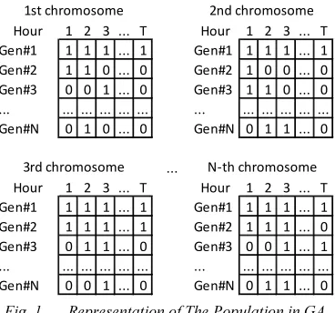
After the generating scheduling result from the PL method is obtained, this result will be used as one of initial population from GA. Then, GA with binary coded will be used to solve this UC problem. The binary coded used in this method are 0 and 1 value which indicate the status of generating unit (0 if the unit is down and 1 if the unit is up). The matrix used for solving this UC problem is three-dimensional matrix with rows represent the scheduling time, columns represent the number of generating units, and the last arrays represent the population size so that if n populations are used, then the last arrays will amount to n. The detail can be seen in Fig. 1.

To get the best individual through the selection process, besides the result from the PL, the initial population must be formed beforehand. This initial population is formed randomly. After the formation process is done, there will be a repaired scheduling to fulfill the minimum up/down time constraints so that the formed initial population is a viable solution. The repaired scheduling steps are as follows,

- If at t-hour the generating unit is down but at (t-1)-hour it is up, then the up time will be checked first. If the up time is over than or equal to the minimum up time of the corresponding unit, then the unit can be shutdown. However, if the minimum up time is not fulfilled yet, then the unit will still be up in the t-hour.

ISSN: 1992-8645 www.jatit.org E-ISSN: 1817-3195

corresponding unit, then the unit can be started up. However, if the minimum down time is not fulfilled yet, then the unit will still be down in the t-hour.

Fig. 1. Representation of The Population in GA

With this repaired scheduling, the initial population which satisfies the minimum up/down time constraints will be obtained. The next process is called the chromosomes evaluation. In this process, the constraints are checked. First, the spinning reserve constraint will be checked at each hour using the schedule from the initial population. If there is a violated spinning reserve in an hour, then the penalty count will be added to the penalty function.

Second, the minimum up/down time must be satisfied so that the individual can enter the ELD problem. If those constraints can’t be satisfied, the individual will be given a penalty count. After the ELD problem is solved, each individual will enter the fitness function calculation process. The penalty count will be multiplied by penalty factor and the penalty function is expressed as in (13). This penalty function, start-up cost, and fuel cost which are obtained from the ELD problem will be summed to obtain the fitness value from each individual inside this population. The formulation can be seen in (14).

function penaltyfactor penalty count

penalty = × . (13)

After calculation of the fitness function is done, the next is the selection process. In this process, there are several sub-parts of the process. The first one is the elitism process. In this process, the best individual will be duplicated so that it won’t enter the next selection process which has the possibility to damage it. This best individual will be kept to be used in the next generation.

Fig. 2 The Illustration of Crossover Process.

function penalty t fuel startup Fitness

cos

cost 1

+ +

=

(14)

The next process is the reproduction process. In this process, there are three sub-processes i.e. parents search, cross over, mutation, and additional operator. The details of how to implement these operators into GA can be seen in the next section. 3.1.1 Parents search

The parents search in GA use the roulette wheel method. Individual whose fitness value bigger than the others will have a bigger chance to be selected. 3.1.2 Cross over

The cross over process is shown in Fig. 2. In this sub-process, the genes on both individual parents will be exchanged based on the cross over point. This sub-process will be run if the randomized number is less than or equal to the cross over probability.

3.1.3 Mutation

In this sub-process, the gene will be mutated if the randomized number is less than or equal to the mutation probability. If the gene is 1, then after this sub-process, it will be changed into 0 and vice versa. This mutation process can be illustrated in Fig. 3.

Fig. 3 The Illustration of Mutation Process.

1 0 0 0 1 1 1 1 1

0 1 0 1 1 0 1 0 0

1 0 0 1 1 1 1 0 0

0 1 0 0 1 0 1 1 1

parents

offsprings

cross over points

1 0 0 0 1 0 1 0 1

1 0 0 1 1 1 1 0 0

mutated

Hour 1 2 3 ... T Hour 1 2 3 ... T

Gen#1 1 1 1 ... 1 Gen#1 1 1 1 ... 1

Gen#2 1 1 0 ... 0 Gen#2 1 0 0 ... 0

Gen#3 0 0 1 ... 0 Gen#3 1 1 0 ... 0

... ... ... ... ... ... ... ... ... ... ... ...

Gen#N 0 1 0 ... 0 Gen#N 0 1 1 ... 0

...

Hour 1 2 3 ... T Hour 1 2 3 ... T

Gen#1 1 1 1 ... 1 Gen#1 1 1 1 ... 1

Gen#2 1 1 1 ... 1 Gen#2 1 1 1 ... 0

Gen#3 0 1 1 ... 0 Gen#3 0 0 1 ... 1

... ... ... ... ... ... ... ... ... ... ... ...

Gen#N 0 0 1 ... 0 Gen#N 0 1 1 ... 0

3rd chromosome N-th chromosome

Fig. 4 Ilustration of Window-mutation for Best Chromosome Operator

3.1.4 Additional operator

Besides these three sub-processes, there are additional operators applied to the individuals i.e. window, window-mutation, and the swap-mutation as well as the swap-window-hill-climb for the best chromosome [13]. These additional operators are used to produce a more optimal solution. Beside of these operators, there are two additional operators that run only for the best chromosome in every generation. These operators are introduced so that the optimal solution can be found. These operators, both for the best chromosome, are window-mutation and mutation-hour. The details of how to implement these operators into GA can be seen in the next sub-section.

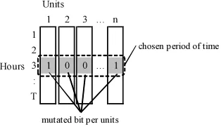
Fig. 5 Ilustration of Mutation-hour for Best Chromosome Operator

3.1.4.1 Window-mutation for best chromosome The window-mutation operator is applied to the best chromosome with the probability of one. It generates a random value of 0 or 1 with equal probability. Then, it selects one unit at random and a “time window” of width w equal to MDT (if random value is 0) or MUT (if random value is 1) of the corresponding unit. After that, this operator

is run from the 1st hour to the (T+1-w)th hour to mutate the bits in that window to 0s if w equal to MDT or 1s if w equal to MUT. If this task produces a better solution, this solution will be kept. Otherwise, it will be restored to the solution before this task is performed. The illustration can be seen in Fig. 4.

3.1.4.2 Mutation-hour for best chromosome This operator is also applied to the best chromosome with the probability of 0.7. It selects one of a period time randomly. After that, this operator is run from the 1st unit until the Nth unit to mutate one bit of each unit. If this task produces a better solution, this solution will be kept. Otherwise, it will be restored to the solution before this task is performed. The illustration can be seen in Fig. 5.

After this process is done, a new population with different chromosomes is formed. It will re-enter the fitness function process, the selection process, and so on until the maximum generation is reached. The best individual at the last generation will become the solution of this UC problem.

3.2 Lambda Iteration for Solving ELD Problem

In this ELD problem, the objective function is to minimize the fuel cost which is represented by quadratic function. The penalty function is added to the objective function by summing it with the fuel cost. This new function, after added by the penalty terms, is called the Lagrange function. The minimum condition will be obtained by (15) [1].

( )

dP P dF

i i

i _{, i 1 to}

= =λ

. (15)

i i

i _a

b P

2 − =

λ

. (16)

λ is the incremental cost value of all units. From (15), the formulation can be modified into (16) to get the value of the generated power from each unit. If there are generating units at their limits, this direct solution can’t work well so that the lambda iteration method is used to solve this ELD problem. In lambda iteration, λ is searched using iteration. The method starts with two values of lambda, below and above the optimal value, then it will iterate until the absolute difference of two lambdas is less than the convergence tolerance. To include the inequality constraint i.e. the generating limits in

hours

units 1 2 3 4 5 6 7 … … … T

1

2

3 0 0 0 0

: : :

n

hours

units 1 2 3 4 5 6 7 … … … T

1

2

3 1 1 1 1

: : :

n

OR

w indow

w indow

rand=0

rand=1

Units

1 2 3 … n

1

2

Hours 3 1 0 0 … 1

:

T

chosen period of time

ISSN: 1992-8645 www.jatit.org E-ISSN: 1817-3195

lambda iteration, the formulation in (17) are used in each iteration [1].

i i

i i

i i

i i

P P

P P P

P P P

min, max,

min, max,

) ( for

) ( for , )

(

, )

(

< >

= =

λ λ

λ λ

. ₍₁₇₎

The flowchart to solve these problems can be seen in Fig. 6.

After the generated power results from the ELD problem are obtained, the fuel cost can be calculated and will be used in the calculation of the fitness function process.

Fig. 6 Flowchart of The Proposed Method.

4. SIMULATION RESULTS

This proposed method is implemented in Matlab program and tested on 10-units-system case study and its duplication.

4.1 Case 1: 10 Units System

Table I: Comparison of GABPL Method among Other Methods on 10 Units System

Method

Total start-up

cost ($)

Total fuel cost

($)

Total operational cost

($)

PSO [15] - - 574,153

DE [16] 4780 568,262.6 573,042.6

HPSOGA [17] - - 568,960

ICGA [4] - - 566,404

MA [18] - - 565,827

LR [13] - - 565,825

GA [13] - - 565,825

DPSO [7] 2095 562,899 565,804

SPL [19] - - 564,950

LRGA [20] - - 564,800

TSRP [21] - - 564,551

MRCGA [22] - - 564,244

DP combined

with PL [23] - - 564,049

ACO [5] - - 564,049

UCCGA [24] - - 563,977

PL EA [8] 4090 559,887 563,977

MPL [3] 4090 559,887 563,977

HPSO [25] - - 563,942

SFLA [7] 4090 559,847.7 563,937.7

GABPL 4090 559,847.7 563,937.7

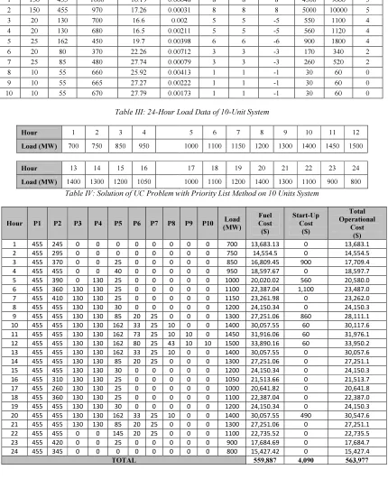
In this case, the spinning reserve is specified as 10% from load [7]. The data is taken from [10] and can be seen in Table II and Table III. The GA parameters used in this case are optimized using DOE method [12]. The optimal values of these parameters are obtained for population size of 30 with maximum generation of 200, crossover probability 0.7, and mutation probability 0.12. With these parameters, the best obtained total cost is $563,937.7. This result is then compared to the total cost results from other methods in the reference papers shown in Table I.

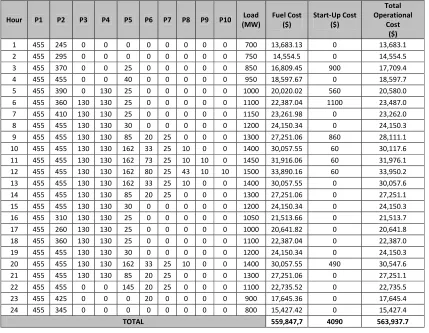
First, the GABPL result can be compared with the PL result on 10 units test system. The PL result on 10 units test system can be seen from Table IV and the GABPL best result can be seen in

Table V. The total cost obtained by this PL result is $563,977. With this result, the GABPL method can decrease the total cost as much as $40 to become $563,937.7. Unit 5at 23th hour with 25 MW generated power is turned off and unit 6 is turned on. Because the minimum generated power in unit 6 is 20 MW, 5 MW less than unit 5’s, it can be generated by unit 2 so that the total generated power from unit 2, previously 420 MW, become 425 MW.

From Table I, it can be seen that the obtained total cost of the proposed method is lower than the

Randomly initialize population

Population repairing

Chromosomes evaluation Input generation scheduling from PL result into 1st_{population in GA}

Solved UC with PL based on APC

Penalty=0? Penalty= penalty+1

Solving ELD problem using lambda iteration No

Yes

Calculation of fitness function

Selection process: 1. Parents search 2. Cross over 3. Mutation 4. Additional operators

Generation>max generation?

Finish No

other methods like differential evolution (DE), integer coded GA (ICGA), TS random perturbation (TSRP), memetic algorithm (MA), DP combined with PL, dynamic PSO (DPSO), hybrid PSO (HPSO), hybrid PSO and GA (HPSOGA), unit characteristic classification GA (UCCGA), stochastic PL (SPL), LRGA, LR, GA, PL EA, and methodological PL (MPL). This proposed method produces the most minimal total cost along with the SFLA [7]. This proposed method can get better solution because of better initial population. The improved PL as one of initial population can make GA to converge better compare to usual GA method. The proposed method has as much as 1,887.3$ reducing cost compare to usual GA method [13] in 10 unit system.

4.2 Case 2: The Duplications of 10 Units System

In this case, the generator and loads data are duplicated from the previous case study into 20, 40, 60, 80, and 100 units systems. The spinning reserve used in these test systems is specified as 10% from the load too. The maximum generations used in these systems are 300, 300, 500, 500, and 500 respectively. Because of the stochastic nature of metaheuristic method, this proposed method is run 10 times in every case study. The average total costs obtained in each case study as well as its comparison to other methods can be seen in Table VI. The average cost of proposed method on 20, 40, 60, 80, and 100 unit test systems are $563,941; $1,124,293; $2,246,375; $3,366,134; $4,488,750; $5,607,773 respectively. The obtained total cost on 20 unit test system is not twice more expensive than total cost on 10 unit test system, because there is other way to obtain lower total cost. It can be done by maximizing the power generated from cheaper generation unit or turning on cheaper generation unit so that lower total cost can be obtained.

From Table VI, it can be seen that, on 20 and 40 units systems, the total costs obtained by GABPL method is still higher than SFLA but lower than the other systems (60, 80, and 100 units system). Compared to PL EA method, the total costs obtained by GABPL method are lower on 10, 20, and 100 units systems. Overall, the application of the proposed method to large test system also gives better average total cost compared to other methods.

5. CONCLUSION

The UC problem is an important problem that has to be solved in electrical power system,

especially in system generation. It consists of two sub problems, namely generation scheduling problem and economic dispatch problem. With optimizing the generation scheduling and economic dispatch problem, it can save great amount of cost. So, when optimization can decrease small amount of cost, it will be great advantage. Because of the inadequacy of conventional methods in solving large UC problem, metaheuristic methods are being studied. Researcher also developed hybrid method which combines several methods to get a better solution.

GABPL method with additional operator to solve the UC problem is presented in this paper. This is the hybrid method which is incorporating improved PL as one of initial population in GA. This approach can make GA obtain a better

minimum value with faster convergence.

Comparison of the results to other methods in 10 units test system indicates that the proposed method gives better solution than the other methods. In obtaining average total cost for large system, the proposed method can generate better average total cost than the other methods. It can be concluded that this proposed method is good in finding solution of the UC problem.

In this paper, GABPL method is only tested to common UC problem. There is no emission constraint, reliability constraint, or other constraint that can be included in the UC problem to make the UC modeling more realistic. In future work, we can include these constraints to UC problem to see the performance of this method.

REFERENCES:

[1] A. J. Wood and B. F. Wollenberg, Power Generation, Operation, and Control, 2nd ed., vol. 37. New York: John Wiley & Sons, Inc, 1996, p. 569.

[2] N. P. Padhy, “Unit commitment-a

bibliographical survey,” IEEE Trans. Power Syst., vol. 19, no. 2, pp. 1196–1205, May 2004.

[3] Y. Tingfang and T. O. Ting, “Methodological Priority List for Unit Commitment Problem,”

2008 Int. Conf. Comput. Sci. Softw. Eng., no. 2, pp. 176–179, 2008.

[4] I. Damousis, “A solution to the unit-commitment problem using integer-coded genetic algorithm,” IEEE Trans. Power Syst., vol. 19, no. 2, pp. 1165–1172, 2004.

[5] T. Sum-im and W. Ongsakul, “Ant colony search algorithm for unit commitment,” in

IEEE International Conference on Industrial Technology, 2003, 2003, vol. 1, pp. 72–77. [6] Z.-L. Gaing, “Discrete particle swarm

ISSN: 1992-8645 www.jatit.org E-ISSN: 1817-3195

in IEEE Power Engineering Society General Meeting 2003, 2003, vol. 1, pp. 418–424. [7] J. Ebrahimi, “Unit commitment problem

solution using shuffled frog leaping algorithm,” IEEE Trans. Power Syst., vol. 26, no. 2, pp. 573–581, 2011.

[8] D. Srinivasan and J. Chazelas, “A priority list-based evolutionary algorithm to solve large scale unit commitment problem,” in 2004 International Conference on Power System Technology, 2004. PowerCon 2004., 2004, vol. 2, pp. 1746–1751.

[9] T. Senjyu, K. Shimabukuro, K. Uezato, and T. Funabashi, “A fast technique for unit commitment problem by extended priority list,” IEEE Trans. Power Syst., vol. 18, pp. 882–888, 2003.

[10] W. Chang and X. Luo, “A solution to the unit commitment using hybrid genetic algorithm,” in TENCON 2008 - 2008 IEEE Region 10 Conference, 2008, pp. 1–6.

[11] G. Sheblé, T. Maifeld, and K. Brittig, “Unit commitment by genetic algorithm with penalty methods and a comparison of Lagrangian search and genetic algorithm—economic dispatch example,” Int. J. Electr. Power Energy Syst., vol. 18, no. 6, pp. 339–346, 1996.

[12] Sarjiya, A. B. Mulyawan, A. Setiawan, and A. Sudiarso, “Thermal unit commitment solution using genetic algorithm combined with the principle of tabu search and priority list method,” in 2013 International Conference on Information Technology and Electrical Engineering (ICITEE), 2013, pp. 414–419. [13] S. Kazarlis, A. Bakirtzis, and V. Petridis, “A

genetic algorithm solution to the unit commitment problem,” IEEE Trans. Power Syst., vol. 11, no. February, pp. 83–92, 1996. [14] V. N. Dieu and W. Ongsakul, “Ramp rate

constrained unit commitment by improved priority list and augmented Lagrange Hopfield network,” Electr. Power Syst. Res., vol. 78, no. 3, pp. 291–301, Mar. 2008.

[15] B. Zhao, C. X. Guo, B. R. Bai, and Y. J. Cao, “An improved particle swarm optimization algorithm for unit commitment,” Int. J. Electr. Power Energy Syst., vol. 28, pp. 482–490, 2006.

[16] M. Govardhan and R. Roy, “An application of Differential Evolution technique on unit commitment problem using Priority List approach,” in 2012 IEEE International Conference on Power and Energy (PECon), 2012, no. December, pp. 2–5.

[17] S. M. H. Hosseini, H. Siahkali, and Y. Ghalandaran, “Thermal Unit Commitment

Using Hybrid Binary Particle Swarm

Optimization and Genetic Algorithm,” in 2012 Asia-Pacific Power and Energy Engineering Conference, 2012, no. 2, pp. 1–5.

[18] J. Valenzuela and A. E. Smith, “A seeded memetic algorithm for large unit commitment problems,” J. Heuristics, vol. 8, pp. 173–195, 2002.

[19] T. Senjyu, T. Miyagi, A. Y. Saber, N. Urasaki, and T. Funabashi, “Emerging solution of

large-scale unit commitment problem by Stochastic Priority List,” Electr. Power Syst. Res., vol. 76, pp. 283–292, 2006.

[20] C. Cheng, C. Liu, and C. Liu, “Unit commitment by Lagrangian relaxation and genetic algorithms,” IEEE Trans. Power Syst., vol. 15, pp. 707–714, 2000.

[21] T. A. A. Victoire and A. E. Jeyakumar, “Unit commitment by a tabu-search-based hybrid-optimisation technique,” IEE Proceedings - Generation, Transmission and Distribution, vol. 152. p. 563, 2005.

[22] L. Sun, Y. Zhang, and C. Jiang, “A matrix real-coded genetic algorithm to the unit commitment problem,” Electr. Power Syst. Res., vol. 76, pp. 716–728, 2006.

[23] W. Ongsakul and N. Petcharaks, “Unit

Commitment by Enhanced Adaptive

Lagrangian Relaxation,” IEEE Trans. Power Syst., vol. 19, pp. 620–628, 2004.

[24] T. Senjyu, H. Yamashiro, K. Uezato, and T. Funabashi, “A unit commitment problem by using genetic algorithm based on unit characteristic classification,” 2002 IEEE Power Eng. Soc. Winter Meet. Conf. Proc. (Cat. No.02CH37309), vol. 1, 2002.

Table II: Generator Data of 10-Unit System

Unit P min (MW)

P max (MW)

Fuel Cost Coefficients _MUT (h)

MDT (h)

Init cond.

(h)

Hot SUC ($)

Cold SUC ($)

Τ Cold

($) a ($/MW2_{) b ($/MW) c ($)}

1 150 455 1000 16.19 0.00048 8 8 8 4500 9000 5

2 150 455 970 17.26 0.00031 8 8 8 5000 10000 5

3 20 130 700 16.6 0.002 5 5 -5 550 1100 4

4 20 130 680 16.5 0.00211 5 5 -5 560 1120 4

5 25 162 450 19.7 0.00398 6 6 -6 900 1800 4

6 20 80 370 22.26 0.00712 3 3 -3 170 340 2

7 25 85 480 27.74 0.00079 3 3 -3 260 520 2

8 10 55 660 25.92 0.00413 1 1 -1 30 60 0

9 10 55 665 27.27 0.00222 1 1 -1 30 60 0

10 10 55 670 27.79 0.00173 1 1 -1 30 60 0

Table III: 24-Hour Load Data of 10-Unit System

Hour 1 2 3 4 5 6 7 8 9 10 11 12

Load (MW) 700 750 850 950 1000 1100 1150 1200 1300 1400 1450 1500

Hour 13 14 15 16 17 18 19 20 21 22 23 24

Load (MW) 1400 1300 1200 1050 1000 1100 1200 1400 1300 1100 900 800

Table IV: Solution of UC Problem with Priority List Method on 10 Units System

Hour P1 P2 P3 P4 P5 P6 P7 P8 P9 P10 Load (MW)

Fuel Cost ($)

Start-Up Cost

($)

Total Operational

Cost ($)

1 455 245 0 0 0 0 0 0 0 0 700 13,683.13 0 13,683.1

2 455 295 0 0 0 0 0 0 0 0 750 14,554.5 0 14,554.5

3 455 370 0 0 25 0 0 0 0 0 850 16,809.45 900 17,709.4 4 455 455 0 0 40 0 0 0 0 0 950 18,597.67 0 18,597.7 5 455 390 0 130 25 0 0 0 0 0 1000 20,020.02 560 20,580.0 6 455 360 130 130 25 0 0 0 0 0 1100 22,387.04 1,100 23,487.0 7 455 410 130 130 25 0 0 0 0 0 1150 23,261.98 0 23,262.0 8 455 455 130 130 30 0 0 0 0 0 1200 24,150.34 0 24,150.3 9 455 455 130 130 85 20 25 0 0 0 1300 27,251.06 860 28,111.1 10 455 455 130 130 162 33 25 10 0 0 1400 30,057.55 60 30,117.6 11 455 455 130 130 162 73 25 10 10 0 1450 31,916.06 60 31,976.1 12 455 455 130 130 162 80 25 43 10 10 1500 33,890.16 60 33,950.2 13 455 455 130 130 162 33 25 10 0 0 1400 30,057.55 0 30,057.6 14 455 455 130 130 85 20 25 0 0 0 1300 27,251.06 0 27,251.1 15 455 455 130 130 30 0 0 0 0 0 1200 24,150.34 0 24,150.3 16 455 310 130 130 25 0 0 0 0 0 1050 21,513.66 0 21,513.7 17 455 260 130 130 25 0 0 0 0 0 1000 20,641.82 0 20,641.8 18 455 360 130 130 25 0 0 0 0 0 1100 22,387.04 0 22,387.0 19 455 455 130 130 30 0 0 0 0 0 1200 24,150.34 0 24,150.3 20 455 455 130 130 162 33 25 10 0 0 1400 30,057.55 490 30,547.6 21 455 455 130 130 85 20 25 0 0 0 1300 27,251.06 0 27,251.1 22 455 455 0 0 145 20 25 0 0 0 1100 22,735.52 0 22,735.5 23 455 420 0 0 25 0 0 0 0 0 900 17,684.69 0 17,684.7 24 455 345 0 0 0 0 0 0 0 0 800 15,427.42 0 15,427.4

ISSN: 1992-8645 www.jatit.org E-ISSN: 1817-3195

Table V: Solution of UC Problem with Proposed Method on 10 Units System

Hour P1 P2 P3 P4 P5 P6 P7 P8 P9 P10 Load (MW)

Fuel Cost ($)

Start-Up Cost ($)

Total Operational

Cost ($)

1 455 245 0 0 0 0 0 0 0 0 700 13,683.13 0 13,683.1

2 455 295 0 0 0 0 0 0 0 0 750 14,554.5 0 14,554.5

3 455 370 0 0 25 0 0 0 0 0 850 16,809.45 900 17,709.4 4 455 455 0 0 40 0 0 0 0 0 950 18,597.67 0 18,597.7 5 455 390 0 130 25 0 0 0 0 0 1000 20,020.02 560 20,580.0 6 455 360 130 130 25 0 0 0 0 0 1100 22,387.04 1100 23,487.0 7 455 410 130 130 25 0 0 0 0 0 1150 23,261.98 0 23,262.0 8 455 455 130 130 30 0 0 0 0 0 1200 24,150.34 0 24,150.3 9 455 455 130 130 85 20 25 0 0 0 1300 27,251.06 860 28,111.1 10 455 455 130 130 162 33 25 10 0 0 1400 30,057.55 60 30,117.6 11 455 455 130 130 162 73 25 10 10 0 1450 31,916.06 60 31,976.1 12 455 455 130 130 162 80 25 43 10 10 1500 33,890.16 60 33,950.2 13 455 455 130 130 162 33 25 10 0 0 1400 30,057.55 0 30,057.6 14 455 455 130 130 85 20 25 0 0 0 1300 27,251.06 0 27,251.1 15 455 455 130 130 30 0 0 0 0 0 1200 24,150.34 0 24,150.3 16 455 310 130 130 25 0 0 0 0 0 1050 21,513.66 0 21,513.7 17 455 260 130 130 25 0 0 0 0 0 1000 20,641.82 0 20,641.8 18 455 360 130 130 25 0 0 0 0 0 1100 22,387.04 0 22,387.0 19 455 455 130 130 30 0 0 0 0 0 1200 24,150.34 0 24,150.3 20 455 455 130 130 162 33 25 10 0 0 1400 30,057.55 490 30,547.6 21 455 455 130 130 85 20 25 0 0 0 1300 27,251.06 0 27,251.1 22 455 455 0 0 145 20 25 0 0 0 1100 22,735.52 0 22,735.5 23 455 425 0 0 0 20 0 0 0 0 900 17,645.36 0 17,645.4 24 455 345 0 0 0 0 0 0 0 0 800 15,427.42 0 15,427.4

TOTAL 559,847,7 4090 563,937.7

Table VI: Comparison of GABPL Method among Other Methods on 10 Units System and the Duplications

Number of units

Total Operational Cost ($) GABPL

(average)

PL EA

[8] EPL [9]

SFLA

[7] GA [13] LR [13]

ICGA

[4] EP [8] BF [7]

SPL

[19]

10 563941 563977 563977 564769 565825 565825 566404 564551 564842 564950

20 1124293 1124295 1124369 1123261 1126243 1130660 1127244 1125494 1124892 1123938

40 2246375 2243913 2246508 2246005 2251911 2258503 2254123 2249093 2246223 2248645

60 3366134 3363892 3366210 3368257 3376625 3394066 3378108 3371611 3369237 3371178

80 4488750 4487354 4489322 4503928 4504933 4526022 4498943 4498479 4491287 4492909