Full Length Article
A novel adaptive genetic algorithm for global optimization of
mathematical test functions and real-world problems
M.J. Mahmoodabadi
⇑
, A.R. Nemati
Department of Mechanical Engineering, Sirjan University of Technology, Sirjan, Iran
a r t i c l e i n f o
Article history:Received 28 May 2016 Revised 19 October 2016 Accepted 24 October 2016 Available online 2 November 2016
Keywords:
Adaptive genetic algorithm Particle swarm optimization Sliding mode control Test functions Oil demand estimation
a b s t r a c t
Genetic algorithm (GA) is a population-based stochastic optimization technique that has two major prob-lems, i.e. low convergence speed and falling down in local optimum points. This paper introduces an adaptive genetic algorithm (AGA) consisting of new crossover and mutation operators to handle these drawbacks. The crossover operator is based on a combination of the traditional crossover mechanism and the particle swarm optimization (PSO) operator. The proposed mutation operator intelligently uses sliding mode control (SMC) to escape from local minimums and converges to the global optimum. The performance of the proposed genetic algorithm is challenged by using twenty well-known test functions. The comparison of the obtained numerical results with those of the other optimization algorithms reported in literature demonstrates the superiority of the proposed algorithm in finding the global opti-mum points. At the end, the proposed method is employed to estimate the oil demand in Iran based on socio-economic indicators and using linear and exponential forms as a real-world problem that shows the AGA’s effectiveness.
Ó2016 Karabuk University. Publishing services by Elsevier B.V. This is an open access article under the CC BY-NC-ND license (http://creativecommons.org/licenses/by-nc-nd/4.0/).
1. Introduction
In the most general terms, the optimization theory is a body of
mathematical results and numerical methods to find and identify
the best candidate from a collection of alternatives without having
to explicitly enumerate and evaluate all possible ones
[1]
.
Nowa-days, it is fully accepted that optimization is widely applied in
dif-ferent branches of science, industry and commerce
[2–5]
. Many
real-world optimization problems in engineering are increasingly
becoming complicated, so optimization algorithms with high
per-formance are needed
[6,7]
. Optimization algorithms have
devel-oped and evolved rapidly in recent years leading to reduced
computation times and the improved accuracy of desired results.
Moreover, evolutionary optimization algorithms specially the
Genetic algorithm (GA) and particle swarm optimization (PSO)
have attracted much attention of many researches. Usually, they
have combined the optimization algorithms together to use their
advantages simultaneously
[8–10]
. Shieh et al. combined PSO with
Simulated Annealing (SA) by a proper procedure for parameters
selection to improve the solution quality than SA and fast the
searching ability than PSO
[11]
. Kiran et al. incorporated PSO with
Ant Colony Optimization (ACO) and proposed the hybrid ant
parti-cle optimization algorithm to find the global minimum
[12]
. In
their algorithm, PSO and ACO work separately in each iteration
and the obtained best solutions are applied to select the new
posi-tion of particles and ants at the next iteraposi-tion. Moradi and Abedini
suggested a new combined GA and PSO for optimal Distributed
Generation (DG) location and sizing on distribution systems
[13]
.
Mahmoodabadi et al. also proposed a novel fuzzy combination of
PSO and GA for Pareto optimal design of a five-degree of freedom
vehicle vibration model
[14]
. Akpinar et al. presented a novel
hybrid of ACO and GA for a mixed-model assembly line balancing
problem with some particular traits of real world problems
[15]
. In
a different work, Örkcü offered a new hybrid algorithm based on
adaptive genetic and simulated annealing algorithms for the
vari-able selection problem of multiple linear regression models
[16]
.
Valdez et al. proposed a novel hybrid procedure based on PSO
and GA that uses the fuzzy logic to integrate the results of the
two algorithms
[17]
. Kuo et al. also described a new hybrid
approach in which global best and particle best solutions of PSO
are combined with crossover and mutation operators of GA
[18]
.
In these studies
[11–18]
, the numerical results have been obtained
for general and simple test functions, and compared with pure
optimization algorithms, and not tested for complicated problems.
http://dx.doi.org/10.1016/j.jestch.2016.10.012
2215-0986/Ó2016 Karabuk University. Publishing services by Elsevier B.V.
This is an open access article under the CC BY-NC-ND license (http://creativecommons.org/licenses/by-nc-nd/4.0/).
⇑
Corresponding author.E-mail addresses:[email protected],[email protected]
(M.J. Mahmoodabadi).
Peer review under responsibility of Karabuk University.
Contents lists available at
ScienceDirect
Engineering Science and Technology,
an International Journal
Further, GA premature convergence to the local optimum is an
undesirable phenomenon often reported in literature
[19–21]
.
Many researchers have shown that by using an adaptive mutation
one could overcome this issue. For instance, Tang and Tseng
sug-gested a simple adaptive directed mutation for real-coded GA
[22]
. Their proposed operator uses the abilities of GAs in searching
global optima as well as in speeding convergence by integrating
results of local directional and adaptive random search strategies.
Linda and Nair gave a new GA by employing an adaptive mutation
strategy for optimization of a global multi-machine power system
stabilizer
[23]
. Alfi presented a PSO-based optimization technique
with two new aspects, namely an adaptive mutation mechanism
and a dynamic inertia weight, in order to enhance the global search
ability and to increase accuracy
[24]
. Wang et al. proposed a PSO
variant with new adaptive mutation to escape particles from local
optimal and solve multimodal optimization problems
[25]
.
In the present research, an adaptive genetic algorithm (AGA) is
proposed that its crossover operator named GB-crossover uses a
new composition of the traditional crossover of GA and the global
best position of PSO. In other words, two chromosomes are
selected for the crossover operator, from the mating pool, one of
them is chosen randomly and the other is the position of the best
particle of the entire swarm. The mutation operator used for the
AGA applies an intelligent algorithm originated from sliding mode
control (SMC) concepts. This innovative mutation operator (named
quasi sliding surface-mutation) gradually decreases the changing
of the genes of the selected chromosome. It also quite prevents
particles from converging towards local optimum points. The
capa-bility of the proposed approach is evaluated on some well-known
benchmark functions and the results are compared with several
recent optimization algorithms applied to the same benchmark
functions. Finally, the AGA is applied to estimate the future oil
demand values in Iran based on population, Gross Domestic
Pro-duct (GDP) and import and export data. In the recent years,
researchers have proposed different approaches for modeling the
energy demand
[26–35]
. Furthermore, Yu and Zhu developed a
PSO-GA optimal model to predict energy demand in China using
Gross Domestic Product (GDP), population, economic structure,
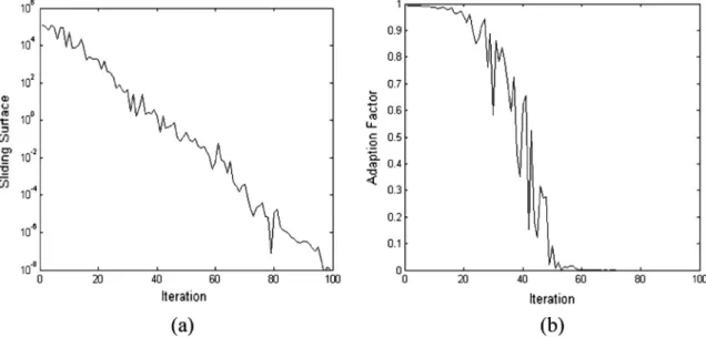
Fig. 1.The obtained trajectory of the sliding surface (a) and the adaptation factor (b) for the Sphere test function.
urbanization rate, and energy structure with linear, exponential
and quadratic forms
[36]
. Kiran et al. presented a novel hybrid
algorithm based on PSO and ACO for energy demand forecasting
in Turkey
[37]
. They supposed that the main affecting factors of
energy demand in Turkey include GDP, population, import and
export. They also applied two new models in order to estimate
electricity energy demand in Turkey by using Artificial Bee Colony
(ABC) and PSO algorithms
[38]
. Further, Yu and Zhu proposed a
hybrid technique (PSO-GA) to improve energy demand estimation
in China by applying linear, exponential, and quadratic models and
considering GDP, population, economic structure, urbanization
rate, and energy consumption structure
[39]
. Piltan et al. used
PSO and GA to attain the parameters of the energy demand
fore-casting model in Iranian metal industry
[40]
. The coefficients of
two linear and three nonlinear functions are optimized by
consid-ering a function of different variables such as electricity tariff,
manufacturing value added, prevailing fuel prices, the number of
employees, the investment in equipment, and consumption.
Ghan-bari et al. presented a cooperative ACO-GA approach to construct a
knowledge-based expert system for simulating fluctuations of
energy demand
[41]
. They evaluate the ability of this algorithm
by applying it on three case studies; annual electricity demand,
natural gas demand and oil products demand in Iran. Rahmani
et al. introduced a new hybrid of ACO and PSO to predict the
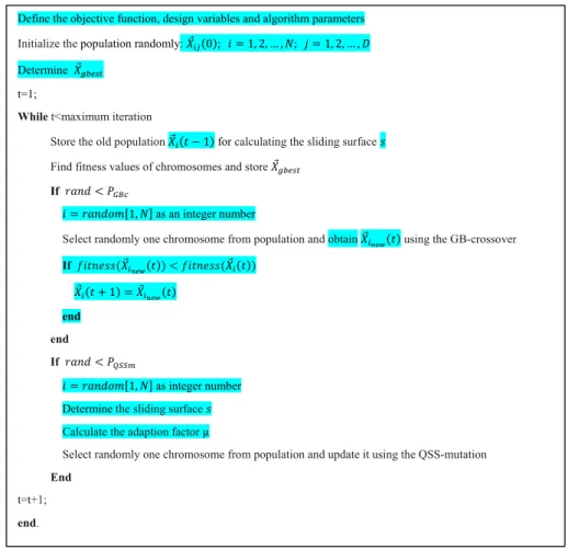
Define the objective function, design variables and algorithm parameters
Initialize the population randomly: (0); = 1, 2, … Determine
t=1;
While t<maximum iteration
Store the old population ( − 1) for calculating the sliding surface Find fitness values of chromosomes and store
If
[1 ] as an integer number
Select randomly one chromosome from population and obtain ( )using the GB-crossover
If ( ( )) ( ( )) ( + 1) = ( ) end end If [1 ] as integer number Determine the sliding surface
Calculate the adaption factor µ
Select randomly one chromosome from population and update it using the QSS-mutation End
t=t+1; end.
Fig. 3.The pseudo code of the AGA.
Table 1
General mathematical test functions used to evaluate the algorithms.
Name Formulation Search domain Globalfmin
Unimodal Sphere f1ðxÞ ¼PD i¼1x2i [100, 100] D 0 Schwefel’s P2.22 f2ðxÞ ¼PD i¼1jxij þ QD i¼1jxij [10, 10] D 0 Schwefel’s P1.2 f3ðxÞ ¼PD i¼1ð Pi j¼1xjÞ 2 [100, 100]D 0 Schwefel’s P2.21 f4ðxÞ ¼maxjxij;i2 ½1:D [100, 100]D 0 Rosenbrock f5ðxÞ ¼PD1 i ½100ðxiþ1x2iÞ 2 þ ðxi1Þ2 [10, 10] D 0 Quaric f6ðxÞ ¼PD i¼1ix4iþrandom½0;1 [1.28, 1.28] D 0 High Conditioned Eliptic
f7ðxÞ ¼PD i¼1ð106Þ i1 D1x2 i [100, 100]D 0 Multimodal Rastrigin f8ðxÞ ¼PD i¼1x2i10 cosð2
p
xiÞ þ10 [5.12, 5.12]D 0 Ackley f9ðxÞ ¼ 20 exp 0:2 ffiffiffiffiffiffiffiffiffiffiffiffiffiffiffiffiffiffiffi 1 D PD i¼1x2i q þ20exp 1 D PD i¼1cosð2p
xiÞ þe [32, 32] D 0 Griewank f10ðxÞ ¼ 1 4000 PD i¼1x2i QD i¼1cos pxiffii þ1 [600, 600]D 0 Weierstrass f11ðxÞ ¼PD i¼1ð PKmax k¼0 akcosð2p
bkðxiþ0:5ÞÞ h i Þ DPKmax k¼0 akcosðp
bkÞ h i a¼0:5;b¼3;Kmax¼20 [0.5, 0.5] D 0energy output of a real wind farm located in Binaloud, Iran with
the meteorological data consisting of the wind speed and the
ambi-ent temperature
[42]
. Askarzadeh compared standard PSO with six
variants of PSO for estimation of the electricity demand in Iran
[43]
.
The rest of this paper is organized as follows. Section
2
gives
briefly an overview of GA, PSO and SMC. Section
3
describes the
operators and structure of the AGA and the ability of this proposed
algorithm for preventing of premature convergence to local
opti-mum points and rapidly converges to the global optiopti-mum. Then,
in Section
4
, well-known general and shifted test functions and
the used algorithms for comparison are illustrated. Furthermore,
simulation results and comparisons on the solution accuracy and
the convergence speed are shown in this section to verify the
suf-ficiency of the AGA. Moreover, this algorithm is implemented to
estimate Iran’s oil demand in Section
5
to indicate the capability
of the presented algorithm for solving the real-world and
con-strained problems. Lastly, Section
6
concludes the paper.
2. Background
2.1. Genetic algorithm
John Holland presented GA in 1975 with the inspiration of
Dar-win’s theoryabout the survival of fittest
[44]
. One of the
capabili-ties of stochastic algorithms is to work over a set of solutions
called population. Each member of the population is called a
chro-mosome
~
X
i¼ ½
x
1;
x
2;
. . .
;
x
Dwhere
D
is the number of gens. The
standard version of the GA is organized by three operators;
repro-duction, crossover, and mutation. After applying these operators,
the new population would be created. This process is iterated until
the stopping criterion is met, and the chromosome with the best
Table 4
Mean, maximum, minimum and standard deviation of the best fitness values for 30 runs found by the AGA, GA-TC, GA-MC, S-PSO and F-GA&PSO for Sphere test function.
Dimension 10 20 30 40 GA-TC mean 2.456105 3.001103 1.158 27.468 maximum 3.386103 2.574101 10.935 46.941 minimum 1.258107 1.858104 9.864102 2.562 std. dev. 9.254106 3.021103 1.646 22.364 GA-MC mean 9.49910+3 3.15810+4 5.61610+4 8.00710+4 maximum 1.19810+4 7.65110+4 9.36210+4 1.54310+5 minimum 8.68710+2 7.78610+3 9.15810+3 2.13910+4 std. dev. 2.84710+3 5.57610+3 7.78810+3 1.09410+4 S-PSO mean 1.79310+3 1.29810+4 3.02210+4 4.99 310+4 maximum 9.76910+3 3.35410+4 5.00710+4 7.72710+4 minimum 5.83410+2 7.07510+3 9.89910+3 1.00610+4 std. dev. 434.875 2.14110+3 2.82710+3 3.82810+3 F-GA&PSO mean 1.6291019 2.9171011 4.671107 1.703104 maximum 1.3851018 3.6451010 4.743106 8.930104 minimum 2.4761023 1.2541015 9.3791012 2.647107 std. dev. 2.1741019 3.2001011 5.321107 2.780104 AGA mean 3.0811099 3.8781060 1.0981043 4.2821035 maximum 3.1771098 7.7021059 1.3871042 5.9951034 minimum 5.58910105 6.2171065 5.1751049 4.5421043 std. dev. 8.6291099 1.4261059 3.4531043 1.4111034 Table 3
Parameter settings for optimization algorithms.
Algorithm Parameter
AGA PGBc¼0:9;PQSSm¼0:1
GA-TC Pr¼0:2;Ptc¼0:4;Pm¼0:1;s¼0:05, the tournament selection method
GA-MC Pr¼0:2;Pmc¼0:4;Pm¼0:1;s¼0:05, the tournament selection method
S-PSO w¼0:9;C1¼C2¼2:0
F-GA&PSO w1¼0:9;w2¼0:4,C1i¼C2f¼2:5;C1f¼C2i¼0:5,
fm¼0:001;ntc¼nmc¼0:2 Table 2
Shifted mathematical test functions used to evaluate the algorithms.
Name Formulation fbias Search domain Global
fmin
Unimodal Shifted Sphere f12ðxÞ ¼PD
i¼1z2iþfbias;zi¼xi0 450 [100, 100] D 450 Shifted Schwefel’s P1.2 f13ðxÞ ¼PD i¼1ð Pi j¼1zjÞ 2 þfbias;zi¼xi0:5 450 [100, 100] D 450
Shifted Schwefel’s P1.2 with
Noise in Fitness f14ðxÞ ¼ ð PD i¼1ð Pi j¼1xjÞ 2 Þð1þ4ðrandom½0;1ÞÞ þfbias;zi¼xi0:5 450 [ - 100, 100] D 450 Shifted High Conditioned
Eliptic f15ðxÞ ¼ PD i¼1ð106Þ i1 D1z2 iþfbias;zi¼xi0 450 [100, 100] D 450 Shifted Rosenbrock f16ðxÞ ¼PD1 i 100ðziþ1z2iÞ 2 þ ðzi1Þ2 h i þfbias;zi¼xiþ1 390 [100, 100] D 390
Multimodal Shifted Rastrigin f17ðxÞ ¼
PD i¼1z2i10 cos 2ð
p
ziÞ þ10 þfbias;zi¼xi0 330 [5, 5] D 330 Shifted Ackley with GlobalOptimum on Bounds f18ðxÞ ¼ 20 exp 0:2
ffiffiffiffiffiffiffiffiffiffiffiffiffiffiffiffiffiffiffi 1 D PD i¼1z2i q þ20exp 1 D PD i¼1cosð2
p
ziÞ þeþfbias;zi¼xi0 140 [32, 32]D 140Shifted Rotated Griewank
without Bounds f19ðxÞ ¼ 1 4000 PD i¼1z2i QD
i¼1cos pziffii þ1þfbias;zi¼ ðxi0:5Þð1þ3 randomð ½0;1ÞÞ
180 [0, 600]D 180 Shifted Weierstrass f20ðxÞ ¼PD i¼1 PKk¼0max akcos 2
p
bkðziþ0:5Þ h i DPKmax k¼0 akcosp
bk h i þfbias;a¼0:5;b¼3;Kmax¼20;zi¼xi1 90 [0.5, 0.5]D 90Table 5
Mean, maximum, minimum and standard deviation of the best fitness values for 30 runs found by the AGA, GA-TC, GA-MC, S-PSO and F-GA&PSO for Schwefel’s P2.22 test function. Dimension 10 20 30 40 GA-TC mean 7.700103 0.058 0.242 1.062 maximum 5.364102 0.476 1.002 12.419 minimum 1.021105 7.598104 9.436103 5.858102 std. dev. 2.100103 0.013 0.068 0.510 GA-MC mean 51.427 5.85010+5 5.45110+10 5.30910+15 maximum 1.95310+2 4.86410+6 7.84210+11 8.95310+16 minimum 4.497 2.37010+3 5.92310+8 5.96410+10 std. dev. 48.268 1.48310+6 2.06710+11 2.68210+16 S-PSO mean 10.132 43.007 841.197 6.74210+6 maximum 21.075 72.096 1.35610+4 5.35410+7 minimum 1.007 9.972 212.065 9.89210+4 std. dev. 1.600 5.631 1.55710+3 1.52710+7 F-GA&PSO mean 3.3461011 6.696107 1.784104 7.103103 maximum 3.9471010 6.724106 1.043103 5.643102 minimum 4.4211014 7.1211010 9.361107 5.515105 std. dev. 2.3321011 4.294107 1.608104 6.596103 AGA mean 1.0051057 3.2221039 2.0361031 1.5221026 maximum 1.6391056 1.7981038 1.3431030 1.9591025 minimum 1.0301060 2.2951041 1.0081032 4.1851028 std. dev. 3.0381057 4.9971039 2.8191031 3.6151026 Table 6
Mean, maximum, minimum and standard deviation of the best fitness values for 30 runs found by the AGA, GA-TC, GA-MC, S-PSO and F-GA&PSO for Schwefel’s P1.2 test function.
Dimension 10 20 30 40 GA-TC mean 2.500103 6.400103 0.019 0.042 maximum 3.553102 7.774102 0.307 0.908 minimum 5.546105 9.610105 7.746104 3.497103 std. dev. 8.800103 0.017 0.079 0.102 GA-MC mean 0.495 0.897 1.428 1.281 maximum 1.598 2.037 3.135 3.213 minimum 0.042 0.121 0.837 0.756 std. dev. 1.037 1.585 2.253 2.532 S-PSO mean 5.148105 1.437104 1.928104 2.683104 maximum 5.590104 9.346104 2.127104 9.386103 minimum 6.125108 1.021107 9.739107 1.205106 std. dev. 1.016104 3.581104 4.488104 5.727104 F-GA&PSO mean 2.273106 7.491106 9.836106 1.939105 maximum 6.754104 9.409104 1.114103 3.463103 minimum 3.7591010 8.0871010 9.9081010 1.212109 std. dev. 8.212106 1.898105 2.131105 6.194105 AGA mean 6.843105 8.536105 1.217104 1.477104 maximum 1.543103 6.104104 5.112103 1.692103 minimum 1.632109 6.952109 4.721109 8.204109 std. dev. 2.215104 1.492104 5.953104 2.921104 Table 7
Mean, maximum, minimum and standard deviation of the best fitness values for 30 runs found by the AGA, GA-TC, GA-MC, S-PSO and F-GA&PSO for Schwefel’s P2.21 test function. Dimension 10 20 30 40 GA-TC mean 0.027 7.978 14.790 19.571 maximum 0.124 17.953 21.603 32.052 minimum 0.010 0.693 2.493 7.987 std. dev. 0.079 3.163 3.248 3.525 GA-MC mean 54.347 75.910 82.907 86.07 maximum 77.903 84.076 90.047 98.128 minimum 27.975 50.092 72.860 79.075 std. dev. 8.355 6.081 4.642 3.386 S-PSO mean 24.545 52.349 64.470 72.483 maximum 52.974 66.426 73.947 87.091 minimum 2.351 21.856 40.032 64.632 std. dev. 3.205 3.876 3.415 3.021 F-GA&PSO mean 7.038108 0.022 1.671 7.775 maximum 8.087107 0.947 5.547 14.087 minimum 8.3581010 2.574106 8.230106 4.359103 std. dev. 5.983108 0.016 0.711 2.037 AGA mean 2.7421031 1.022105 17.102 67.269 maximum 5.3351030 3.044104 57.377 92.522 minimum 4.3541037 1.1191015 3.243106 1.443103 std. dev. 9.9981031 5.557105 31.169 32.036
Table 8
Mean, maximum, minimum and standard deviation of the best fitness values for 30 runs found by the AGA, GA-TC, GA-MC, S-PSO and F-GA&PSO for Rosenbrock test function.
Dimension 10 20 30 40 GA-TC mean 6.776 35.700 1.12810+2 2.18410+2 maximum 9.470 1.14710+2 2.24410+2 3.73810+2 minimum 6.446 17.348 29.877 1.11010+2 std. dev. 1.473 28.578 54.056 61.833 GA-MC mean 1.38010+5 1.15510+6 2.24410+6 3.42710+6 maximum 9.76810+5 8.26810+6 1.46010+7 5.90310+7 minimum 1.24610+3 9.77510+3 1.55510+4 3.43110+4 std. dev. 8.68410+4 3.47610+5 5.60110+5 9.31510+5 S-PSO mean 5.39210+3 2.06010+5 7.52510+5 1.55410+6 maximum 1.05910+4 1.35810+6 1.46010+7 5.90310+7 minimum 1.20510+3 7.87910+3 2.47610+4 2.87610+4 std. dev. 2.61710+3 5.64910+4 1.52810+5 2.24010+5 F-GA&PSO mean 1.216 27.191 44.751 72.775 maximum 5.615 77.000 1.3610+2 2.19110+2 minimum 0.072 0.050 16.747 33.675 std. dev. 1.403 25.861 31.557 39.207 AGA mean 6.317 16.843 27.034 37.194 maximum 6.874 17.352 27.648 37.534 minimum 5.822 15.921 26.483 36.448 std. dev. 0.253 0.283 0.293 0.274 Table 9
Mean, maximum, minimum and standard deviation of the best fitness values for 30 runs found by the AGA, GA-TC, GA-MC, S-PSO and F-GA&PSO for Quaric test function.
Dimension 10 20 30 40 GA-TC mean 3.213103 9.307103 0.020 0.038 maximum 3.465102 9.233102 0.123 0.404 minimum 3.450104 9.980104 3.764103 8.359103 std. dev. 1.313103 3.121103 5.727103 0.011 GA-MC mean 5.709 64.711 183.880 393.701 maximum 14.976 72.987 197.770 402.394 minimum 1.201 17.086 121.898 330.359 std. dev. 3.430 19.510 49.780 80.690 S-PSO mean 0.971 12.416 65.551 176.087 maximum 3.987 21.212 77.970 212.900 minimum 0.006 0.120 11.910 144.801 std. dev. 0.367 3.357 11.417 24.575 F-GA&PSO mean 1.941103 7.149103 0.019 0.038 maximum 2.121102 7.771102 0.212 0.444 minimum 1.110104 6.899104 4.110103 9.992103 std. dev. 9.772104 2.668103 6.771103 0.011 AGA mean 2.797104 7.067104 2.041103 2.266103 maximum 1.452103 1.903103 8.143103 5.753103 minimum 1.506105 6.421105 3.783104 2.930104 std. dev. 2.905104 4.436104 1.719103 1.503103 Table 10
Mean, maximum, minimum and standard deviation of the best fitness values for 30 runs found by the AGA, GA-TC, GA-MC, S-PSO and F-GA&PSO for High Conditioned Eliptic test function. Dimension 10 20 30 40 GA-TC mean 0.560 3.93210+2 1.41310+4 1.14210+5 maximum 2.009 3.23310+3 5.63110+4 2.79010+5 minimum 0.090 32.961 1.71210+3 2.97610+4 std. dev. 0.430 5.82110+2 1.22910+4 6.57810+4 GA-MC mean 7.15010+7 6.11810+8 1.52710+9 2.53810+9 maximum 1.46210+8 1.01810+9 2.61710+9 3.74410+9 minimum 1.18310+7 3.29910+8 8.17510+8 1.15110+9 std. dev. 3.53210+7 1.86810+8 4.40910+8 6.89110+8 S-PSO mean 3.13010+6 6.06910+7 2.34010+8 5.30810+8 maximum 7.41610+6 8.72610+7 3.64610+8 7.54710+8 minimum 1.21110+6 2.84710+7 1.54110+8 3.19610+8 std. dev. 1.55510+6 1.42910+7 4.89710+7 1.02010+8 F-GA&PSO mean 1.7071015 3.298107 1.047102 6.031 maximum 8.4361015 1.442106 4.127102 19.665 minimum 4.7291017 1.585108 1.281103 0.581 std. dev. 2.2591019 3.451107 8.417103 4.868 AGA mean 3.16410111 3.4571069 9.8491052 3.5051041 maximum 9.28110110 7.8511068 2.7481050 9.7581040 minimum 5.40810119 1.9371076 1.0491058 5.6571048 std. dev. 1.69310110 1.4341068 5.0101051 1.7811040
Table 11
Mean, maximum, minimum and standard deviation of the best fitness values for 30 runs found by the AGA, GA-TC, GA-MC, S-PSO and F-GA&PSO for Rastrigin test function.
Dimension 10 20 30 40 GA-TC mean 6.300 14.698 25.394 36.837 maximum 17.953 25.876 34.098 44.871 minimum 0.874 7.890 18.987 21.112 std. dev. 3.136 4.920 7.610 9.225 GA-MC mean 97.526 251.950 410.879 569.759 maximum 121.001 297.009 444.245 601.007 minimum 21.998 40.980 99.071 111.923 std. dev. 10.615 21.889 24.508 29.148 S-PSO mean 52.982 173.939 309.696 448.241 maximum 110.005 212.330 313.086 491.060 minimum 2.758 14.986 35.091 72.946 std. dev. 6.727 10.973 12.281 18.188 F-GA&PSO mean 3.704 14.359 32.959 59.409 maximum 17.990 21.005 39.343 73.222 minimum 0.017 0.123 0.990 2.983 std. dev. 1.738 4.867 8.725 14.198 AGA mean 0 0 3.978109 3.506101 maximum 0 0 1.193107 10.520 minimum 0 0 0 0 std. dev. 0 0 2.178108 1.920 Table 12
Mean, maximum, minimum and standard deviation of the best fitness values for 30 runs found by the AGA, GA-TC, GA-MC, S-PSO and F-GA&PSO for Ackley test function.
Dimension 10 20 30 40 GA-TC mean 0.067 1.550 2.783 4.045 maximum 0.761 12.998 17.998 19.001 minimum 5.513105 1.865103 8.991103 1.911102 std. dev. (0.277) (0.956) (0.959) (1.058) GA-MC mean 18.854 20.053 20.387 20.478 maximum 21.004 21.954 22.002 22.861 minimum 17.087 19.154 19.900 20.020 std. dev. 0.761 0.374 0.290 0.294 S-PSO mean 12.834 17.769 19.020 19.553 maximum 14.001 19.007 21.213 21.650 minimum 1.970 12.870 14.768 15.000 std. dev. 1.186 0.586 0.299 0.237 F-GA&PSO mean 1.6131010 0.115 0.590 1.209 maximum 8.5601010 0.359 0.791 3.130 minimum 9.9861011 0.097 0.127 0.576 std. dev. 1.3551010 0.115 0.745 0.833 AGA mean 4.4401015 6.2171015 7.6381015 9.4141015 maximum 7.9931015 7.9931015 1.5091014 1.5091014 minimum 1.8811015 4.4401015 4.4401015 4.4401015 std. dev. 1.3191015 1.8061015 1.9451015 3.3111015 Table 13
Mean, maximum, minimum and standard deviation of the best fitness values for 30 runs found by the AGA, GA-TC, GA-MC, S-PSO and F-GA&PSO for Griewank test function.
Dimension 10 20 30 40 GA-TC mean 0.063 0.032 0.674 1.457 maximum 0.344 0.211 1.003 3.013 minimum 4.232107 7.812104 7.241103 0.072 std. dev. 0.067 0.052 0.236 0.543 GA-MC mean 86.440 285.253 506.544 721.645 maximum 100.654 310.657 536.096 976.871 minimum 12.346 47.987 97.818 138.054 std. dev. 25.765 50.200 70.092 98.450 S-PSO mean 15.584 122.104 273.025 445.451 maximum 21.875 146.086 303.936 490.043 minimum 3.870 21.087 86.900 110.072 std. dev. 4.192 16.454 26.019 44.027 F-GA&PSO mean 0.108 9.772103 2.917103 8.541105 maximum 1.870 0.881 0.034 8.251104 minimum 3.974103 9.341105 1.943105 7.961107 std. dev. 0.056 0.033 0.021 7.100105 AGA mean 4.121102 3.621103 0 0 maximum 3.345101 1.086101 0 0 minimum 0 0 0 0 std. dev. 2.489102 1.983102 0 0
Table 14
Mean, maximum, minimum and standard deviation of the best fitness values for 30 runs found by the AGA, GA-TC, GA-MC, S-PSO and F-GA&PSO for Weierstrass test function.
Dimension 10 20 30 40 GA-TC mean 0. 752 2.395 5.391 10.786 maximum 0.833 2.553 5.971 11.301 minimum 0.701 2.312 4.645 10.353 std. dev. 0.070 0.136 0.678 0.479 GA-MC mean 9.193 24.247 39.784 60.062 maximum 9.324 25.983 41.107 60.896 minimum 9.088 23.248 37.885 59.018 std. dev. 0.120 1.509 1.686 0.956 S-PSO mean 6.690 22.625 37.551 54.815 maximum 7.813 23.620 38.183 55.488 minimum 5.330 21.878 37.223 54.253 std. dev. 1.258 0.896 0.547 0.624 F-GA&PSO mean 1.371103 2.425102 0.701 2.216 maximum 4.114103 6.159102 1.024 3.166 minimum 1.561108 1.708103 0.238 1.214 std. dev. 2.375103 3.257102 0.411 0.977 AGA mean 0 0 0 0 maximum 0 0 0 0 minimum 0 0 0 0 std. dev. 0 0 0 0 Table 15
Mean, maximum, minimum and standard deviation of the best fitness values for 30 runs found by the AGA, GA-TC, GA-MC, S-PSO and F-GA&PSO for shifted Sphere test function.
Dimension 10 20 30 40 GA-TC mean 449.9999837745328 449.9972976720476 448.4499163144820 420.4920911387130 maximum 449.9999588066938 449.9931744325014 442.8819511247692 388.1314662592574 minimum 449.9999966502348 449.9990235218959 449.8730327580137 442.1867204606277 std. dev. 1.026105 1.546103 1.518 13.093 GA-MC mean 830.8271206286860 3094.207702924056 5641.599439114948 8274.321337189026 maximum 1514.509529036338 4110.281953857641 7442.622749401216 1009.078179111214 minimum 247.8552583488984 1918.299086586165 3626.586856353388 5714.100661851109 std. dev. 3.11810+3 5.50210+3 9.49310+3 9.73410+3 S-PSO mean 1182.494874960175 1316.767566124047 2994.365504144866 4.812075560223211 maximum 2218.564717591757 1652.536751461939 3490.325122363107 5.451251571649575 minimum 301.9667875124316 874.8863270600046 2249.261854790727 3.554409650249442 std. dev. 4.78210+2 2.08410+3 3.02910+3 4.63510+3 F-GA&PSO mean 450 449.9999999999440 449.9999995251106 449.9997860481680 maximum 450 449.9999999994244 449.9999979520674 449.9991817488010 minimum 450 449.9999999999972 449.9999999318787 449.9999844329565 std. dev. 0 1.1881010 4.539107 2.105104 AGA mean 450 450 450 450 maximum 450 450 450 449.9999999999999 minimum 450 450 450 450 std. dev. 0 0 0 3.9491014 Table 16
Mean, maximum, minimum and standard deviation of the best fitness values for 30 runs found by the AGA, GA-TC, GA-MC, S-PSO and F-GA&PSO for shifted Schwefel’s P1.2 test function. Dimension 10 20 30 40 GA-TC mean 449.9993829874049 449.9980536071201 449.9925408112686 449.9077783918694 maximum 449.9982201126205 449.9974226101959 449.9776724346482 449.7873248307561 minimum 449.9999993741910 449.9990732585442 449.9999999634825 449.9960312315511 std. dev. 1.007103 8.913104 1.287102 0.108 GA-MC mean 449.6486380943293 448.8685346225282 449.4291628332339 449.2532590634946 maximum 449.0614807525150 446.6620793665169 448.4741922241739 449.0007699389189 minimum 449.9568529485293 449.9964717689761 449.9201180985775 449.5160109335621 std. dev. 0.508 1.911 0.827 0.257 S-PSO mean 449.9999910054258 449.9999659474472 449.9998652270189 449.9998414362930 maximum 449.9999793767399 449.9999402643471 449.9996435574347 449.9996813116705 minimum 449.9999987666490 449.9999942560277 449.9999886529012 449.9999698307262 std. dev. 1.025105 2.709105 1.923104 1.468104 F-GA&PSO mean 449.9999978871052 449.9999966405426 449.9999955258148 449.9999824102650 maximum 449.9999939847133 449.9999908661935 449.9999875822466 449.9999337437559 minimum 450 450 449.9999999990837 450 std. dev. 2.344106 4.549106 5.089106 2.794105 AGA mean 449.9999959360885 449.9999921236908 449.9999960810008 449.9999880772277 maximum 449.9999707487508 449.9999474812837 449.9999863454146 449.9999431427385 minimum 449.9999999602784 449.9999999919742 449.9999999937223 449.9999999975880 std. dev. 9.039106 1.626105 5.807106 2.512105
fitness would be introduced as the optimal solution. The details of
the reproduction, crossover, and mutation operators are described
in the following.
Reproduction:
In a simple way, two members of the population
are selected randomly then the member with less fitness is
removed from the population and the one with more fitness is
put in place. This operator is done for (P
rN) members of the
population.
P
rand
N
are the probability of the reproduction
and the size of the population, respectively.
Crossover:
A crossover operator selects two members of the
population randomly. Then, it creates two new chromosomes
and puts them at the place of the old chromosomes. The
cross-over operator is usually applied to a number of pairs
deter-mined as (P
tcN)/2, where
P
tcand
N
are the probability of
the crossover and the population size, respectively. Let
~
X
ið
t
Þ
and
~
X
jð
t
Þ
be two randomly selected chromosomes and
~
X
ið
t
Þ
has the smaller fitness value than
~
X
jð
t
Þ
, then the crossover
rela-tions are as follows.
~
X
ið
t
þ
1
Þ ¼
~
X
ið
t
Þ þ
~
c
1ð
~
X
ið
t
Þ
~
X
jð
t
ÞÞ
~
X
jð
t
þ
1
Þ ¼
~
X
jð
t
Þ þ
~
c
2ð
~
X
ið
t
Þ
~
X
jð
t
ÞÞ
ð
1
Þ
where
~
c
1and
~
c
22 ½
0
;
1
Dare random vectors.
Mutation:
Mutation operator causes variations on the values of a
number of chromosomes in the population (determined as
P
mN, where
P
mand
N
are the probability of the mutation
and the population size, respectively). Let
~
X
ið
t
Þ
a randomly
selected chromosome, and then the mutation formulation is
defined as:
~
X
ið
t
þ
1
Þ ¼
~
X
ið
t
Þ þ ð
~
b
g
Þ
ð
2
Þ
where
~
b
2 ½
0
;
1
Dis a random vector and
g
is a constant value.
2.2. Particle swarm optimization
In the PSO algorithm
[45]
, the position vector
~
U
ið
t
Þ
is changed
by adding a velocity vector
~
v
ið
t
Þ
to it as follows
Table 17
Mean, maximum, minimum and standard deviation of the best fitness values for 30 runs found by the AGA, GA-TC, GA-MC, S-PSO and F-GA&PSO for shifted Schwefel’s P1.2 test function with noise in fitness.
Dimension 10 20 30 40 GA-TC mean 449.9985646936117 449.9995366580214 449.9768482611706 449.8689327193002 maximum 449.9973857109426 449.9989148703982 449.9320490211749 449.6109926351037 minimum 449.9988366510013 449.9999325471117 449.9994119744920 449.9846700225463 std. dev. 1.407103 5.627104 3.894102 0.223 GA-MC mean 449.9186438791738 446.4141073209536 449.9544126604372 449.7128661887552 maximum 449.8147846442799 441.2545801124971 449.9298434911697 449.4688667139914 minimum 449.9900004053890 449.8147561449861 449.9996427847039 449.9745888937195 std. dev. 0.070 3.846 0.039 0.253 S-PSO mean 449.9999284658217 449.9999885284668 449.9998138476615 449.9999437261948 maximum 449.9998117567730 449.9999780811913 449.9994285900362 449.9997224890036 minimum 449.9999995133398 449.9999960390725 449.9999420414245 449.999963152574 std. dev. 1.054104 9.332106 3.508104 1.626104 F-GA&PSO mean 449.9999950023186 449.9999990451206 449.9999968631385 449.9999923693189 maximum 449.9999840194949 449.9999952698601 449.9999905894156 449.9999863195532 minimum 449.9999999999784 450 450 449.9999994119204 std. dev. 7.092106 2.110106 5.433106 6.602106 AGA mean 449.9999996303929 449.9999989551646 449.9999999262753 449.9999996911625 maximum 449.9999985214742 449.9999956029188 449.9999997946533 449.9999991521398 minimum 449.9999999951697 449.9999999998866 449.9999999995843 449.9999999972478 std. dev. 6.279107 1.892106 8.275108 4.682107 Table 18
Mean, maximum, minimum and standard deviation of the best fitness values for 30 runs found by the AGA, GA-TC, GA-MC, S-PSO and F-GA&PSO for shifted High Conditioned Eliptic test function with noise in fitness.
Dimension 10 20 30 40 GA-TC mean 89.800120311823065 44.785659135786744 6175.906660381945 9678.863028581396 maximum 0 0 30879.53330190972 48394.31514290698 minimum 449.0006015591154 223.9282956789337 0 0 std. dev. 2.00710+2 1.00110+2 1.380910+4 2.16410+4 GA-MC mean 95038613.62111142 628139467.1060340 1183655090.315825 2668993846.784902 maximum 166548699.3689040 842993720.4283164 1781170337.972066 3447049174.110232 minimum 19262053.58890160 378705600.2122736 718784314.9118657 1798963434.666303 std. dev. 6.01610+7 2.10210+8 4.44710+8 6.80110+8 S-PSO mean 4024464.947335149 47643637.75159591 194539391.7604014 530961373.5759113 maximum 6619122.049961107 63723089.21787029 262225505.6660125 691997922.2474580 minimum 2866912.949787115 24933497.00746602 141578937.2758800 393195819.7200962 std. dev. 1.55910+6 2.02210+7 6.16510+7 1.50710+8 F-GA&PSO mean 450 449.9999987344112 449.9879738051980 444.5714916245727 maximum 450 449.9999925130472 449.9635396521812 431.1295022914000 minimum 450 449.9999999183896 449.9980208697401 448.8713572043769 std. dev. 0 2.229106 0.011 5.441 AGA mean 450 450 450 450 maximum 450 449.9999999999999 449.9999999999999 449.9999999999999 minimum 450 450 450 450 std. dev. 0 1.0551014 2.1111014 4.3521014
~
U
ið
t
þ
1
Þ ¼
U
~
ið
t
Þ þ
~
v
ið
t
þ
1
Þ
ð
3
Þ
~
v
ið
t
þ
1
Þ ¼
w
x
~
v
ið
t
Þ þ
C
1~
r
1ð
U
~
pbesti~
U
ið
t
ÞÞ þ
C
2~
r
2ð
~
U
gbest~
U
ið
t
ÞÞ
ð
4
Þ
where C
1, C
2and
w
are the cognitive learning factor, social learning
factor and inertia weight, respectively.
~
U
pbestiis the personal best
position of the particle
i.
~
U
gbestis the position of the best particle
within the swarm, and
~
r
1,
~
r
22 ½
0
;
1
dare random vectors where
d
is dimension.
2.3. Sliding mode control
The sliding mode controller is a powerful control strategy
applied to robust handle of nonlinear systems
[46–55]
. In this
sec-tion, the general concepts of SMC for a second-order dynamic
sys-tem defined by the following state-space equation are described.
_
x
¼
f
ð
h
;
u
;
t
Þ
ð
5
Þ
where
h
2
R
nis the state vector,
u
2
R
mis the input vector, and
t
is
the time. The sliding surface
s
ð
e
;
t
Þ
is defined as:
s
ð
e
;
t
Þ ¼
d
dt
þ
k
e
¼
0
ð
6
Þ
s
¼
e
_
þ
k
e;
e
¼
h
h
dð
7
Þ
where
k
is a strictly positive constant and
h
dis the desired state
vec-tor. In fact,
s
is a sum-weighted of the position and velocity errors.
In this control method, by changing the control law according to
certain predefined rules which depend on the position of state
errors of the system with respect to sliding surfaces, the states
are switched between stable and unstable trajectories until they
reach the sliding surface
[55]
.
Table 20
Mean, maximum, minimum and standard deviation of the best fitness values for 30 runs found by the AGA, GA-TC, GA-MC, S-PSO and F-GA&PSO for shifted Rastrigin test function. Dimension 10 20 30 40 GA-TC mean 323.9613956917980 313.9139387095056 305.3315578704945 295.1801946529780 maximum 319.0522968263761 298.0720932223101 285.9633972995544 268.0650434297603 minimum 329.0033923519364 323.9469696783326 318.5657942558461 310.7506211122298 std. dev. 2.624 7.027 6.340 9.577 GA-MC mean 231.9698052931943 83.941368063095069 70.760317929220861 236.1408259510231 maximum 212.4165576083890 53.885011698788048 111.8040067233131 276.5894158248347 minimum 262.5106046824117 123.9854940309564 26.133970258747922 150.8674398598100 std. dev. 12.938 18.654 20.148 30.619 S-PSO mean 277.1768516616635 153.0470626955032 32.783281161176426 101.7092016372488 maximum 268.1007442226782 139.6359702847255 16.531704151738040 133.8456720051392 minimum 288.2437691151679 162.1774641862251 58.313023008207892 20.859000129232982 std. dev. 5.430 7.050 13.656 36.315 F-GA&PSO mean 326.3145780230623 315.7467701788274 295.6464454608587 268.8474911347565 maximum 322.0403204297655 306.1209888679108 272.4151217728556 236.0237198109013 minimum 329.8819537334009 326.0193383619661 311.9872240480715 299.6417972654198 std. dev. 1.707 4.674 9.346 14.257 AGA mean 330 329.9999999999987 329.4288611416667 327.5174367040779 maximum 330 329.9999999999690 312.8658342597547 283.9127388666287 minimum 330 330 330 330 std. dev. 0 5.7931012 3.128 9.729 Table 19
Mean, maximum, minimum and standard deviation of the best fitness values for 30 runs found by the AGA, GA-TC, GA-MC, S-PSO and F-GA&PSO for shifted Rosenbrock test function. Dimension 10 20 30 40 GA-TC mean 396.7169325292743 669.8500426088053 22201.25716313337 292680.0310020061 maximum 399.5639733800460 1063.760936413901 73595.40483050168e 966506.8051038038 minimum 392.5458839400190 459.4194942689739 3078.850362025212e 59766.56716796412 std. dev. 2.391 2.37810+2 2.25610+4 2.64310+5 GA-MC mean 1312989928.450298 12698736804.81050 20158404514.52971 29239627456.19702 maximum 3641413484.367582 18994422155.75515 31187077254.86490 46485373401.66466 minimum 237833353.0822434 8042887099.252314 9869203003.529253 18724947626.21279 std. dev. 1.04810+9 3.20710+9 5.70110+9 8.60510+9 S-PSO mean 47948530.92204220 1928556741.888466 7095243433.610+7 97580 15345055869.48889 maximum 75216003.65289119 2658482090.983409 9865562889.146740 19289997678.74270 minimum 14707664.63443860 1330601848.694514 4723389491.999683 11864908313.17943 std. dev. 1.835 4.05310+8 1.58010+9 2.66410+9
F-GA&PSO mean 400.7631178052712 423.2722138655833 454.7913176607509 531.0464844829378e
maximum 449.1466581757315 564.7035492755612 531.2735612358079 855.6660029402847 minimum 390.6951831994961 394.6441395009354 415.3489590734728 428.8583860117879 std. dev. 18.230 54.130 38.011 1.23610+2 AGA mean 390.0103693163959 390.0000000000293 390.0000055661383 390.0000000000462 maximum 390.0812110353763 390.0000000002930 390.0000555189113 390.0000000002925 minimum 390 390 390 390.0000000000001 std. dev. 2.560102 9.2651011 1.755105 9.5851011
Table 21
Mean, maximum, minimum and standard deviation of the best fitness values for 30 runs found by the AGA, GA-TC, GA-MC, S-PSO and F-GA&PSO for shifted Ackley test function with global optimum on bounds.
Dimension 10 20 30 40 GA-TC mean 139.9954751841448 138.5374635701375 137.3833104527502 135.6958985337245 maximum 139.9929757117656 136.0417450878459 136.2048541231768 133.7063907814467 minimum 139.9976555619460 139.9800837892175 138.3306921219629 137.3554190074501 std. dev. 1.212103 1.013 0.564 0.980 GA-MC mean 121.1409083448861 119.8299232061201 119.5856638490304 119.4649582920145 maximum 120.2192789849038 119.4096083447712 119.2552438861343 119.2193540349563 minimum 123.0959999329135 120.7758534028307 120.2132778756837 119.9239611136939 std. dev. 0.739 0.334 0.231 0.203 S-PSO mean 119.6054526561096 119.1529554692678 118.9645897540434 118.8646535066549 maximum 119.4424835750159 119.0626933933543 118.8757692849515 118.8032615023607 minimum 119.7493443842990 119.2989478861391 119.0609793345992 118.9783372946030 std. dev. 0.073 0.059 0.056 0.044 F-GA&PSO mean 139.9999999998468 139.9386637254656 139.6363650743944 138.8401343023154 maximum 139.9999999994627 138.1599814760067 137.7790022180207 137.6150003151231 minimum 139.9999999999735 139.9999992741500 139.9999200049385 139.9982777771635 std. dev. 1.1201010 0.335 0.646 0.779 AGA mean 140 139.9999999999993 139.9999999999664 139.9999999996101 maximum 140 139.9999999999899 139.9999999998142 139.9999999974686 minimum 140 139.9999999999999 139.9999999999995 139.9999999999809 std. dev. 2.5311014 1.8121012 4.6091011 5.1011010 Table 22
Mean, maximum, minimum and standard deviation of the best fitness values for 30 runs found by the AGA, GA-TC, GA-MC, S-PSO and F-GA&PSO for shifted rotated Griewank test function without bounds.
Dimension 10 20 30 40 GA-TC mean 179.9825801365417 179.9216607422553 177.6983433953596 168.2485964490810 maximum 179.9477438416087 179.8623381121829 176.2525137511280 157.1037671577080 minimum 179.9999993441533 179.9656428020683 178.5260630896768 175.4867898152660 std. dev. 0.030 0.053 1.256 9.794 GA-MC mean 111.4686797775816 134.0160670343220 420.9536469767337 681.8078396562808 maximum 56.158183775051839 204.4546030053080 446.5056746454128 733.3147163165897 minimum 154.2261958169383 69.201969519069763 396.5079368826565 591.6814377382542 std. dev. 38.412 54.806 18.670 78.317 S-PSO mean 154.1584115072451 8.764564008438990 877.6754105683400 904.7778144006653 maximum 144.9857313017676 50.405065221202250 100.9304347704108 123.7426472312736 minimum 165.9091851052426 34.815108795819953 786.4061470590939 585.0415780198359 std. dev. 10.697 42.643 1.16810+2 3.26310+2 F-GA&PSO mean 179.8943923251610 179.9999999973435 179.9948025577891 179.8576922572178 maximum 179.7920755427302 179.9999999580797 179.8511962884156 179.1465172991599 minimum 180 179.9999999998250 179.9999859612236 179.9832091828384 std. dev. 0.045 7.497109 0.027 0.169 AGA mean 179.9809385148956 179.9808945605819 179.9687126675721 179.9545297792528 maximum 179.8155751363782 179.8705780086872 179.9589673530622 179.9419697746883 minimum 179.9984210554754 179.9905315632542 179.9768199123363 179.9655346905215 std. dev. 0.041 0.021 4.469103 4.939103 Table 23
Mean, maximum, minimum and standard deviation of the best fitness values for 30 runs found by the AGA, GA-TC, GA-MC, S-PSO and F-GA&PSO for shifted Weierstrass test function. Dimension 10 20 30 40 GA-TC mean 90.68243160562338 92.62769869767138 95.62835293704381 99.81133668986833 maximum 90.78207132556143 93.05874425386949 95.76754799404334 101.45077463412084 minimum 90.54257205148032 91.99132366029672 95.37637069053305 98.23230431295631 std. dev. 0.124 0.562 0.218 1.610 GA-MC mean 100.17278603329092 116.04672600049534 131.97931686585904 148.83583247497340 maximum 100.32941099753873 116.24504459299220 133.12709849005102 150.62029191477802 minimum 100.00413481797922 115.71385676948675 131.15002913544846 146.38712996556176 std. dev. 0.162 0.290 1.026 2.193 S-PSO mean 96.99352358606079 112.10121312994039 127.61205531207980 145.34705410945317 maximum 97.32595439980692 113.13443418136816 128.18282685503970 145.72366308886145 minimum 96.33181487399530 110.47705550735766 127.22273409253024 145.06015884251654 std. dev. 0.573 1.423 0.505 0.340 F-GA&PSO mean 90.000000007731160 90.106262709541355 90.577498056046537 92.639861430215703 maximum 90.000000018520836 90.136831048824774 90.828838630791068 93.070974028222338 minimum 90.000000002096073 90.068452113976250 90.247195173366663 91.876795310525438 std. dev. 9.3471.657109 0.034 0.298 0.662 AGA mean 90 90.000000000000981 90.000000000085905 90.305509925165367 maximum 90 90.000000000002899 90.000000000128864 90.916527562355597 minimum 90 90.000000000000028 90.000000000007105 90.000000000225270 std. dev. 0 1.6571012 6.8331011 0.529
3. Adaptive genetic algorithm
In this section, a novel adaptive genetic algorithm is introduced
and the details of the new crossover and mutation operators are
described.
3.1. Global best-crossover
The global best-crossover (GB-crossover) operator chooses two
chromosomes as parents. One of them is selected from the mating
pool randomly and the other one is the best chromosome of the
population that is the same
~
U
gbestof Eq.
(4)
for the PSO approach
[45]
. Then, the selected parents create an offspring which is
replaced with the selected chromosome. Consider
P
GBCas the
prob-ability of GB-crossover and
N
as the population size, then
P
GBCN
is the number of chromosomes selected to promote by the
GB-crossover. Let
~
X
ið
t
Þ
and
~
X
gbestrepresent the selected chromosome
and the global best chromosome respectively. Then, the offspring
is calculated by the following equation.
~
X
ið
t
þ
1
Þ ¼
~
X
gbestþ
~
r
1~
X
gbest~
r
2~
X
ið
t
Þ
ð
8
Þ
where
~
r
1and
~
r
22 ½
0
;
1
Dare random vectors. After calculation of Eq.
(8)
, the superior between
~
X
ið
t
Þ
and
~
X
ið
t
þ
1
Þ
should be selected. In
fact, the position of the produced chromosome by the traditional
crossover operator, Eq.
(1)
, is between the positions of its parents.
But, in GB-crossover, the selection of the global best chromosome
as one of the parents causes that the position of the obtained
off-spring tends toward the best chromosome and it increases the
con-vergence speed.
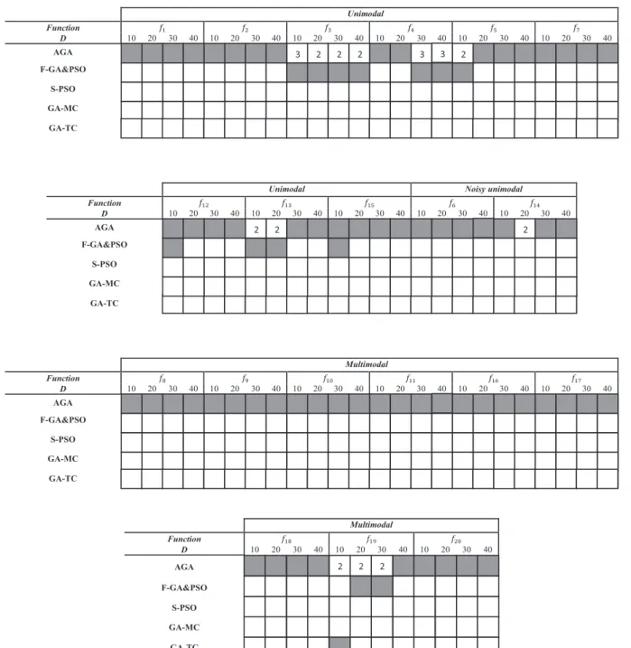
Unimodal Function D 10 20 30 40 10 20 30 40 10 20 30 40 10 20 30 40 10 20 30 40 10 20 30 40 AGA F-GA&PSO S-PSO GA-MC GA-TCUnimodal Noisy unimodal
Function D 10 20 30 40 10 20 30 40 10 20 30 40 10 20 30 40 10 20 30 40 AGA F-GA&PSO S-PSO GA-MC GA-TC Multimodal Function D 10 20 30 40 10 20 30 40 10 20 30 40 10 20 30 40 10 20 30 40 10 20 30 40 AGA F-GA&PSO S-PSO GA-MC GA-TC Multimodal Function D 10 20 30 40 10 20 30 40 10 20 30 40 AGA F-GA&PSO S-PSO GA-MC GA-TC 3 2 2 2 3 3 2 2 2 2 2 2 2
Fig. 4.Indicators of the best test algorithm in the experiments: The cell with grey color represents that the corresponding algorithm outperforms the others for a particular test function at a particular dimension.
3.2. Quasi sliding surface-mutation
The quasi sliding surface-mutation (QSS-mutation) operator
intelligently changes the value of a number of chromosomes in
the population based on the SMC concepts. This number is
deter-mined by
P
QSSmN, where
P
QSSmand
N
are the probability of
QSS-mutation and population size respectively. Let
~
X
ið
t
Þ
is a
ran-domly selected chromosome, then the QSS-mutation is defined
as bellow.
~
X
ið
t
þ
1
Þ ¼
~
X
ið
t
Þ þ ð
~
a
l
Þ
ð
9
Þ
where
~
X
ið
0
Þ
is the initial position and equal to
~
X
ið
1
Þ
,
~
a
2 ½
0
;
1
Dis a
random vector, and the adaptation factor
l
will be calculated by the
following formulation.
l
¼
10
1ffiffiffi
jsj pð
10
Þ
Which
s
¼
e
_
þ
e;
e
¼
f
ð
~
X
ið
t
ÞÞ
; _
e
¼
f
ð
~
X
ið
t
ÞÞ
f
ð
~
X
ið
t
1
ÞÞ
t
ð
t
1
Þ
¼
f
ð
~
X
ið
t
ÞÞ
f
ð
~
X
ið
t
1
ÞÞ
ð
11
Þ
where
f
ð
~
X
ið
t
ÞÞ
is the fitness value of
~
X
ið
t
Þ
and
t
is the iteration
number.
It is observable from Eqs.
(10) and (11)
that if
f
ð
~
X
ið
t
ÞÞ
or
f
ð
~
X
ið
t
ÞÞ
f
ð
~
X
ið
t
1
ÞÞ
are large then the adaptation factor would
be also large. However, if those are small then the adaptation factor
would be small. Hence, QSS-mutation changes the chromosomes
with respect to its fitness value.
Figs. 1 and 2
illustrate this subject
for both unimodal and multimodal test functions; i. e. Sphere and
Griewank (
Table 1
).
3.3. The configuration of the proposed algorithm
The details of the adaptive genetic algorithm are described in
the following. First, the initial population is randomly generated.
After evaluation of the fitness values of all members,
~
X
gbestwould
be determined. Then, according to the values of probabilities
(P
GBcand
P
QSSm), some chromosomes would be randomly selected
to be changed by either GB-crossover or QSS-mutation operators.
This cycle must be repeated until the user-defined stopping
crite-rion is satisfied. The pseudo code of this algorithm is shown in
Fig. 3
.
4. Experimental results on the mathematical test functions
In this section, benchmark functions with experimental tests
are carried out to validate the proposed AGA in comparison with
three other optimization algorithms.
4.1. Mathematical test functions
Twenty well-known general and shifted benchmark problems
with some their essential information are summarized in
Tables
1 and 2 [56,57]
including eleven unimodal test functions and nine
multimodal designed with a considerable amount of local minima
that should be minimized. These general and shifted test functions
are used to evaluate the performance of the AGA, because they are
dimension-wise scalable.
4.2. Algorithms for comparison
In order to validate the performance of the proposed genetic
algorithm, we compare the optimal fitness values found by the
AGA with four other evolutionary algorithms. These algorithms
include GA with Traditional Crossover (GA-TC)
[44]
, GA with
Mul-tiple Crossover (GA-MC)
[58]
, Standard PSO (S-PSO)
[45]
, and Fuzzy
GA and PSO (F-GA&PSO)
[14]
.
4.3. Settings for comparison
The population size is set at 100 for the AGA, GA-TC, GA-MC,
and F-GA&PSO. For standard PSO, the swarm size is considered
as 100. To provide a fair comparison among the test algorithms,
the maximum number of iterations for all algorithms and functions
is fixed at 400. All test functions are tested with dimensions 10, 20,
30, and 40. The performances of the algorithms on each test
func-tion are evaluated based on statistics data obtained from 30
inde-pendent runs. A list of other necessary parameters to run the
algorithms for comparison is stated in
Table 3
.
4.4. Simulation results
At first,
Tables 4–23
show the performance in terms of accuracy
(quality of the averaged optimal fitness) of the AGA on general and
shifted
f
2test functions in comparison with GA-TC, GA-MC, S-PSO,
PSOMS, and F-GA&PSO. They list the average, worst, best and the
standard deviation of the optimal fitness for 30 trials. The bold
val-ues indicate that the corresponding algorithm is the best algorithm
among others on a particular test function at a particular
dimen-sion for mean, maximum and minimum values. It is observable
that the AGA achieves the highest accuracy on functions
f
1,
f
6,
f
7,
f
8,
f
9,
f
10,
f
11,
f
12,
f
15,
f
16,
f
17,
f
18,
f
20at all dimensions. Furthermore,
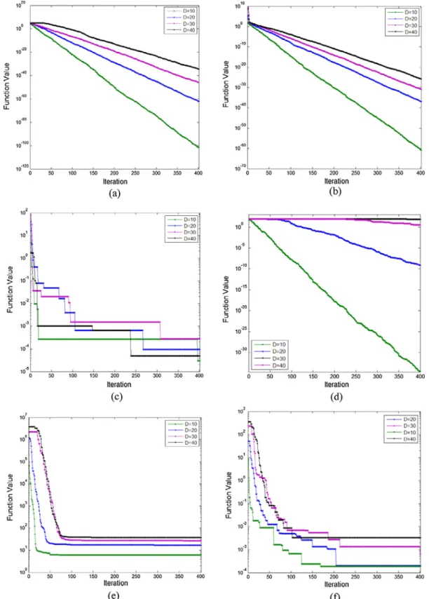
Fig. 6.The evolutionary traces of the AGA on the test functions; (a)f1, (b)f2, (c)f3, (d)f4, (e)f5,(f)f6,(g)f7, (h)f8, (i)f9, (j)f10, and (k)f11for different dimensions;D= 10, 20, 30,
the AGA surpasses all other algorithms in solving functions
f
4for
low dimensions,
f
5,
f
13,
f
14and
f
19for high dimensions.
Fig. 4
shows
a summary of the mean values presented in the previous Tables.
The shaded cells in this figure indicate that the corresponding
algo-rithm is the best on a particular test function at a particular
dimen-sion. When the AGA is not the best algorithm, the numbers inside
the cells indicate its ranking on the relevant test function at the
corresponding dimension. Simply, it can be realized that the AGA
outperforms the other algorithms, because the ranking of the AGA
is the first in 67 cases and is the second with very little differences
in 10 other cases out of a total of 80 cases.
High convergence speed and escaping from local optimum
point for converging to global optimum points are two important
characteristics for an optimization algorithm. In this work, the
GB-crossover operator increases the convergence speed and
QSS-mutation prevents sticking to local optima. The comparisons in
Tables 4–23
and
Fig. 4
show that for both unimodal and
multi-modal problems, the AGA offers the highest accuracy and the best
performance on most test functions. Furthermore, the diversity of
the population shows the ability of the algorithm to escape from
local optimum points. Hence, in this paper, the presented criteria
in Ref.
[59]
named popular standard deviation (psd) as the
follow-ing equation is implemented to evaluate the diversity of the
population.
psd
¼
ffiffiffiffiffiffiffiffiffiffiffiffiffiffiffiffiffiffiffiffiffiffiffiffiffiffiffiffiffiffiffiffiffiffiffiffiffiffiffiffiffiffiffiffiffiffiffiffiffiffiffiffiffiffiffiffiffiffiffiffi
X
N i¼1X
D j¼1x
j ix
j 2"
#
=
ð
N
1
Þ
v
u
u
t
ð
12
Þ
where
N,
D
and
x
are the population size, dimension and the average
position of all chromosomes, respectively.
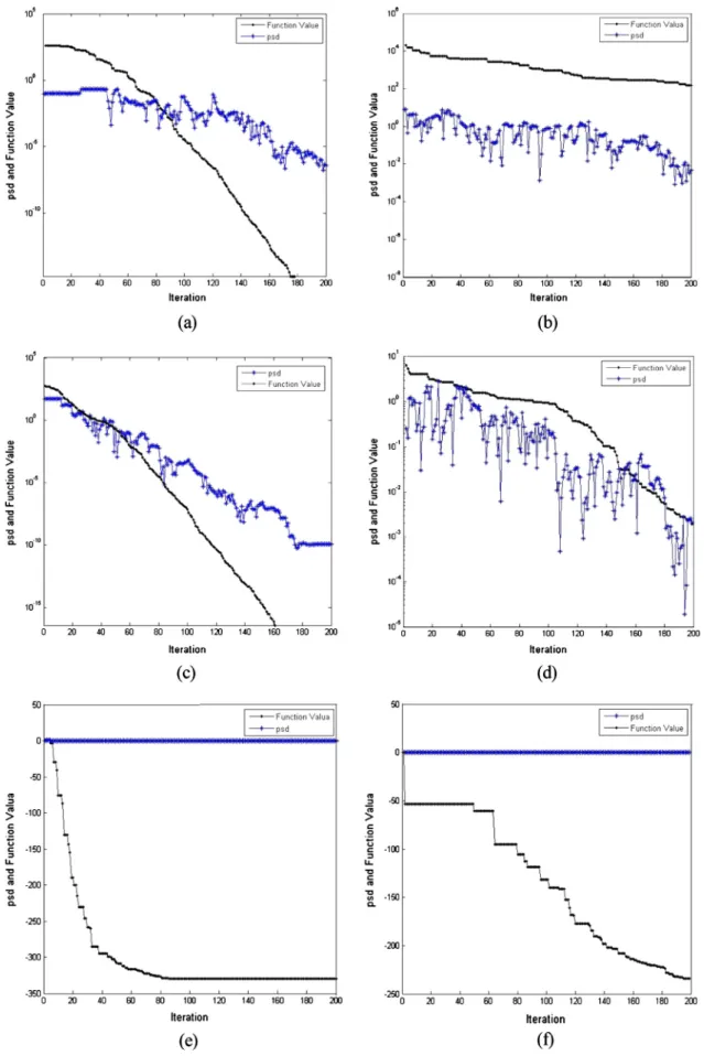
Fig. 5
shows the mean
psd
and function value of the AGA and F-GA&PSO on four
multi-modal test functions for 30 runs. The larger
psd
rather than function
value reflects the high diversity of the population, while small
psd
show that the population is converging to local optimum. This
fig-ure indicate that the mean
psd
of the AGA is larger for test functions
f
8,
f
10, and
f
17in comparison with the mean
psd
of F-GA&PSO. Thus,
the AGA escapes successfully from local optimum points and
con-verges to global optimum point with considering
Table 11, 13 and
20
. Whereas,
Fig. 5
and
Table 22
show that F-GA&PSO is better than
the AGA in test function
f
19with dimension 30.
Fig. 6
describes the evolutionary traces of the general test
func-tions (
Table 1
) and illustrates their mean values at every iteration
for the AGA which are obtained at dimensions (D) 10, 20, 30, and
40 for 30 runs. This figure graphically presents the convergence
characteristics of the evolutionary processes for solving the eleven
different problems and proves that the AGA can successfully jump
out from the local optimum on the test functions. It can be
observed from results comparison that the used techniques and
formulations for the AGA can significantly improve its performance
for finding the global optimal point of an optimization problem.
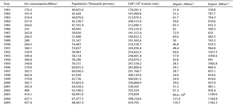
Table 24
Oil demand, GDP, population, import and export data of Iran between 1981 and 2005[60]. Year Oil consumptionðMboeÞa
Population (Thousand persons) GDP (109
Iranian rials) ImportðMboeÞa
ExportðMboeÞa 1981 176.2 40,825.6 170,281.2 21.4 339.8 1982 191.9 42,420 191,666.8 31.2 787.7 1983 234.4 44,076.6 212,876.5 61.7 764.3 1984 257.6 45,720.7 208,515.9 39.6 610.6 1985 264.6 47,541.4 212,686.3 65.3 652.3 1986 241 49,445 193,235.4 62 566.5 1987 262.8 50,650 191,312.4 72.9 635 1988 264.5 51,890 180,822.5 69.6 682.5 1989 280 53,167 191,502.6 50 765.5 1990 284.5 54,483 218,538.7 46.8 919.5 1991 306.1 55,837 245,036.4 48.4 964.8 1992 330.9 56,963 254,822.5 64.6 1023.3 1993 349.4 58,114 258,601.4 57.9 1058.6 1994 366.8 59,290 259,876.3 42.6 991 1995 344.8 59,151 267,534.2 28.5 1002.8 1996 370.9 60,055.5 283,806.6 29.1 880.4 1997 383.5 60,936.5 291,768.7 28.7 855.1 1998 402.8 61,830 300,139.6 24.6 854.6 1999 379.8 62,736 304,941.2 26.9 810.6 2000 382.7 63,663.9 320,068.9 39.6 955.9 2001 392.4 64,528.2 330,565 51.3 901.1 2002 406 65,540.2 355,554 67.3 928.4 2003 414.1 66,991.6 379,838 99.6106 1109.6 2004 427.1 67,477.5 398,234.6 121.6 1184.9 2005 457.4 68,467.4 419,705 116.7 1182.3
aMboe: Million barrel of oil equivalents. 1 barrels of oil equivalent (boe) = 6119 J (J).
Table 25
Maximum and minimum values of the effective parameters used for normalization.
Xmin Xmax
Population (Thousand persons) 40,825.6 62,736
GDP (billion Iranian rials) 170,281.2 304,941.2
Import (Mboe) 21.4 72.9
Export (Mboe) 339.8 1058.6
Oil consumption (Mboe) 176.2 402.8
5. Application of the AGA on demand estimation of oil in Iran
5.1. Problem definition
In this section, in order to challenge the performance of the AGA
for a real-world problem, it has been developed to estimate the
future oil demand values based on population, Gross Domestic
Pro-duct (GDP) and import and export data. For this purpose, the
fit-ness function is considered as follows that should be minimized.
F
ð
x
Þ ¼
X
m j¼1E
actualE
predicted 2ð
13
Þ
where
E
actualand
E
predictedare the actual and predicted oil demand,
respectively, and
m
is the number of observation. The data related
to the effective parameters (Iran’s population, GDP, import, export
and oil consumption) is taken from the energy balance annual
report of the energy ministry of Iran in 2005
[60]
and shown in
Table 12
. Furthermore, the prediction of the oil demand, based on
the socio-economic indicators, is modeled by using an equation
with a new form as follows.
E
predicted¼
w
1þ
w
2X
1þ
w
3X
2þ
w
4X
3þ
w
5X
4þ
w
6exp
ð
w
10X
1Þ þ
w
7exp
ð
w
11X
2Þ þ
w
8exp
ð
w
12X
3Þ þ
w
9exp
ð
w
13X
4Þ
ð
14
Þ
where
X
1,
X
2,
X
3, and
X
4are the normalized value of the population,
GDP, import and export of oil respectively, and
w
i(i
¼
1
;
2
;
3
;
. . .
13
Þ
are the weight coefficient that should be found by the optimization
algorithm. Moreover, the variables of this optimization problem are
constrained as
1
6
w
p6
1
;
p
¼
1
;
2
;
. . .
;
9
w
q6
0
;
q
¼
10
;
11
;
12
;
13
ð
15
Þ
In the other words, the AGA is applied to find optimal values of
weight parameters based on actual data for estimation of the oil
consumption. In order to normalize the population, GDP, import,
export and oil consumption, Eq.
(16)
is applied.
X
N¼ ð
X
RX
minÞ
=
ð
X
maxX
minÞ
ð
16
Þ
where
X
N,
X
R,
X
min, and
X
maxare the normalized value (N
= 1, 2, 3, 4),
the real value (
Table 24
), the minimum and maximum value
(
Table 25
), respectively.
5.2. Estimation of oil demand by using the AGA
The following configurations are considered to perform the
optimization process for the prediction of the oil demand.
Popula-Table 26
Optimum value of the weight coefficients for Eq.(14)by proposed model to predict the oil demand.
Weight coefficient w1 w2 w3 w4 w5 w6 w7 w8 w9 w10 w11 w12 w13 GA-TC +0.3473 +0.2678 +0.7194 0.4092 +0.2459 +0.4576 +0.2910 0.7735 0.3282 0.1299 1.8898 0.7538 0.3527 GA-MC 0.4165 +0.6202 0.2116 +0.0082 0.0421 +0.1347 0.6074 +0.9782 +0.1154 0.2422 1.6632 0.2890 1.1382 S-PSO 0.4083 +0.2024 +0.5414 0.1990 +0.4762 0.0282 +0.1645 +0.6819 0.6102 0.4041 3.5071 0.8345 7.9933 F-GA&PSO +0.2066 +0.6983 +0.2749 0.1130 0.1027 0.4269 0.2957 0.3087 0.0303 0.3166 0.7480 0.8492 4.3880 AGA 0.2447 +0.5290 +0.2200 0.0283 +0.0394 0.0675 0.0048 0.2823 +0.7029 1.3309 0.0537 0.0568 0.1134 Table 27
Comparison of the AGA with actual data, estimated value with other algorithms by proposed model, and predicted values in Ref.[27].
Year 2000 2001 2002 2003 2004 2005 Average
Actual data 382.700 392.400 406.000 414.100 427.100 457.400 –
AGA with the proposed model 383.519 392.254 406.071 419.565 427.069 440.943 –
Relative error of AGA (%) 0.214 0.037 0.018 1.320 0.007 3.598 0.87
F-GA&PSO with the proposed model 372.152 385.370 405.419 421.558 426.974 444.752 –
Relative error of F-GA&PSO (%) 2.756 1.791 0.142 1.801 0.029 2.765 1.547
S-PSO with the proposed model 388.585 392.188 407.130 427.982 433.355 453.694 –
Relative error of S-PSO (%) 1.537 0.053 0.278 3.352 1.464 0.810 1.250
PSO-DEMexponential 384.045 388.317 401.876 421.502 431.958 443.353 –
Relative error of PSO-DEMexponential(%) 0.351 1.041 1.016 1.787 1.137 3.071 1.40
PSO-DEMlinear 386.773 389.436 404.594 425.571 436.778 452.985 –
Relative error of PSO-DEMlinear(%) 1.064 0.755 0.346 2.770 2.266 0.965 1.36
GA-MC with the proposed model 380.515 392.729 405.185 423.983 428.778 431.508 –
Relative error of GA-MC (%) 0.570 0.084 0.200 2.386 0.393 5.660 1.549
GA-TC with the proposed model 391.925 388.236 4.09622 422.831 423.410 467.558 –
Relative error of GA-TC (%) 2.410 1.060 0.892 2.108 0.863 2.220 1.592
GA- DEMexponential 392.103 394.697 413.502 433.202 448.191 469.126 –
Relative error of GA-DEMexponential(%) 2.457 0.585 1.848 4.613 4.938 2.564 2.83
GA-DEMlinear 393.349 390.998 403.335 426.912 437.095 452.484 –
Relative error of GA-DEMlinear(%) 2.783 0.357 0.656 3.094 2.340 1.075 1.72
Fig. 8.Comparison between the actual and predicted values by AGA and Assareh et al.[27]for the oil consumption among years 2000 and 2005.
tion size: 20, Probability of GB-crossover: 0.9, Probability of
SS-mutation: 0.1, Maximum number of iterations: 100.
Fig. 7
shows the evolutionary trace of the estimation of oil
demand obtained via the AGA, and
Table 26
gives the achieved
weight coefficients in proposed model (Eq.
(14)
) at the end of this
process for all algorithms.
Table 27
and
Fig. 8
illustrate the values
of oil demand predicted by using the AGA, from 2000 to 2005. These
values are compared with the actual data, estimated value with
other algorithms by proposed model, and predicted values by
Assareh et al.
[27]
(The bold values indicate the best prediction
for each year). In fact, Assareh et al. utilized two algorithms (genetic
algorithm and particle swarm optimization) and two models (linear
and exponential) for the prediction of the oil demand.
Table 27
depicts that the average relative error of the proposed model
opti-mized by PSO and GA is smaller than linear and exponential models
and the introduced model by this work is a proper model for the
estimation of the oil demand. Furthermore, this table indicates that
the predicted data by AGA based on the proposed model is in a very
good agreement with the actual values in comparison with the
obtained values by other models and algorithms.
6. Conclusion
In this work, a new adaptive genetic algorithm using two novel
operators called GB-crossover and QSS-mutation is presented. In
GB-crossover, the best chromosome from the entire population
(Global Best Chromosome) is utilized as one of the parents which
originated from particle swarm optimization
.
This operator creates
one offspring from two parents in the mating pool. QSS-mutation
changes the value of the selected chromosomes intelligently based
on the sliding mode concept organized from sliding mode control.
To consider the performance of the AGA, it is applied for eleven
unimodal and nine multimodal test functions. The depicted results
are compared with the obtained results from several well-known
and recent optimization algorithms. The comparisons indicate that
the AGA offers the highest accuracy and the best performance on
most unimodal and multimodal test functions. Also, the ability of
the AGA for avoiding being trapped into local optimum points for
multimodal functions is shown. Moreover, the AGA is successfully
used to estimate the oil demand of Iran based on the
socio-economic conditions. Validations of the proposed model show that
it is in a good agreement with regard the observed results and is a
satisfactory tool for successful oil demand forecasting. So, the
obtained results prove that the AGA is verily an effective and
suc-cessful algorithm for optimization of both constrained and
uncon-strained mathematical test functions and real-world problems.
References
[1]A. Ravindran, K.M. Ragsdell, G.V. Reklaitis, Engineering Optimization: Method and Applica
![Fig. 8. Comparison between the actual and predicted values by AGA and Assareh et al. [27] for the oil consumption among years 2000 and 2005.](https://thumb-us.123doks.com/thumbv2/123dok_us/612171.2573357/18.892.63.843.129.222/fig-comparison-actual-predicted-values-assareh-consumption-years.webp)
