Behavioral Simulation Methods in Tax Policy Analysis

(1)

of Economic Research

Volume Title: Behavioral Simulation Methods in Tax Policy Analysis

Volume Author/Editor: Martin Feldstein, ed.

Volume Publisher: University of Chicago Press

Volume ISBN: 0-226-24084-3

Volume URL: http://www.nber.org/books/feld83-2

Publication Date: 1983

Chapter Title: Alternatives to the Current Maximum Tax on Earned Income

Chapter Author: Lawrence Lindsey

Chapter URL: http://www.nber.org/chapters/c7706

Chapter pages in book: (p. 83 - 108)

(2)

3

Alternatives to the

Current Maximum Tax

on Earned Income

Lawrence B. Lindsey

The Maximum Tax on Personal Service Income, passed as a part of the Tax Reform Act of 1969, provides a tax reduction to taxpayers with substantial earned income. However, it does not, as is widely assumed, place a 50% limit on the rate at which earned income is taxed. In an earlier paper (Lindsey 1981) I showed that the vast majority of high- income taxpayers still face marginal tax rates on earned income in excess of 50%.

This paper considers alternatives to the current maximum tax rules which would be more effective at setting a 50% ceiling on the rate at which earned income is taxed. Particular attention is paid to the behavioral response of taxpayers faced with a change in the tax rules.

The simulations contained in this paper are made with the National Bureau of Economic Research TAXSIM model. This model bases its calculations on the 1977 Tax Model File provided by the Internal Rev- enue Service. This data file contains a stratified random sample of individual tax returns; a random sample of 7,703 of these returns was used for this paper.

The data have been aged to reflect 1981 dollar amounts. TAXSIM does this automatically by increasing all dollar items by the percent increase in personal income between the two years. A further adjustment is made to the number of returns in each income class. The TAXSIM estimates of total revenue are within 2% of Department of Treasury revenue estimates for any given tax year.

Lawrence B. Lindsey is tax economist at the Council of Economic Advisers. He is on leave from Harvard University and the National Bureau of Economic Research.

The author is deeply grateful to Martin Feldstein, Richard Musgrave, and Daniel Feenberg, whose comments and criticisms were invaluable. He is also thankful to Jerry Hausman for his suggestions on functional form.

(3)

Four alternatives to the present law are considered. Two of these involve a rewriting of the existing maximum tax rules to more effectively limit the top earned income tax rate to 50%. These alterations as well as existing law create complicated nonlinearities in the tax schedule. The TAXSIM model is designed to generate precise marginal tax rates for both earned and unearned income to take account of these complexities. The third alternative involves a change in the existing statutory rate schedule to make the top tax rate 50% on all income. The fourth alternative considered is abolition of the existing maximum tax altogether and application of the current rate schedule to all income regardless of source.

The methodological emphasis of this paper is on simulating the behavioral response of taxpayers to changes in the tax law. Two types of behavior are considered: changes in effort and changes in tax avoidance. Although a well-established literature exists on the effect of tax rates on labor supply, most of the studies do not include the affluent, the people affected by the reforms considered in this paper. Therefore a range of parameter values for the effects of price and income on effort has been used. The literature on tax avoidance behavior is not well established. I present an empirical estimation of this behavior and am conducting further research on this topic. I use this estimated value as well as a value half as great as that estimated and a parameter value implying no avoidance behavior. The reader is free to make judgments based upon his or her expectations of the actual parameters.

Section 3.1 examines the current maximum tax law and the reasons for its failure to set a top rate on earned income of 50%. Section 3.2 considers alternative tax rules and their revenue cost in the absence of a behavioral response. The excess burden placed on earned income by the different rules is also presented in this section. Section 3.3 discusses the techniques used in simulating taxpayer response to alternative tax rules. Section 3.4 presents the results based on a range of parameter values for the behavioral model.

3.1 The Existing Maximum Tax Provision

Under existing law a taxpayer qualifying' for the maximum tax provision is allowed to subtract from what his or her tax liability otherwise would have been the difference between the ordinary tax liability on earned taxable income and what that liability would have been if a 50% top rate had been imposed. Figure 3.1 illustrates the provision. Without

1. Taxpayers who are married filing separately or who average their income are ineligible for the maximum tax. Furthermore, in order to qualify, the taxpayer must have earned taxable income at least as great as the 50% bracket amount, $60,000 for married taxpayers, $41,700 for single taxpayers.

(4)

85 Alternatives to the Current Maximum Tax on Earned Income

MARGINAL TAX RATE

50% Earned Total TAXABLE INCOME Brocket Taxable Taxable

Amount Income Income Fig. 3.1

the maximum tax the taxpayer’s liability would have been the sum of areas X, Y , and 2. The taxpayer is allowed to subtract the difference between the ordinary liability on earned taxable income (areasxand Y )

and what the liability would have been if a 50% rate had been imposed ( a r e a x ) . In short, the taxpayer receives a tax reduction equal to area Y

and pays tax equal to areas X and 2. The tax due on unearned income (area 2 ) is unaffected by this rule.

However, this is not equivalent to a maximum rate on earned income of 50%. Consider what happens if the taxpayer earns another dollar of taxable income. Without the maximum tax provision he or she would pay

B% on this dollar. The maximum tax provision reduces the tax rate by the difference between what it would have been if the taxpayer had only earned income, A%, and 50%, or a tax rate reduction of ( A - 50)%. Therefore even with the maximum tax, the tax rate on earned income is

( B - A

+

50)%. This rate will exceed 50% unless B% equals A%. Only taxpayers with very large earned income, so that both B and A equal the statutory limit of 70%, and taxpayers with little or no unearned income are in this situation.

A second complication in the maximum tax law which increases the marginal tax rate on earned income above 50% is that only a fraction of

(5)

earned income is treated as earned taxable income for tax purposes. The remainder is taxed at the unearned income rate. If we define F as the fraction of earned income treated as earned taxable income by the maximum tax provision, the marginal tax rate on earned income becomes

F ( B - A + 5 0 ) % + ( 1 - F ) B % .

It is clear that this rate is in excess of 50%, as B > A

>

50. Under existing law F can be computed as

TAXINC + PSINC TAXINC PSINC ~-

AGI AGI AGI AGI

’

where TAXINC is taxable income, PSINC is personal service income, and AGI is adjusted gross income. The reason for this fraction is that deductions must be apportioned between earned and unearned income. The current law apportions deductions to earned income according to the share of earned income in total income. The fraction of each dollar treated as earned income rises both as deductions decline as a share of AGI (taxable income rises as a share of AGI) and as earned income becomes a greater share of AGI.

In summary, the current maximum tax law fails to establish a maximum rate on earned income for two reasons. First, the tax rate on earned taxable income ( B - A

+

50)% depends upon the tax rate levied on the total amount of income received ( B % ) . Second, only a fraction of earned income is treated as earned for tax purposes. In order to achieve a maximum tax rate of 50%, the tax rate on earned taxable income must be independent of B and thus independent of the total amount of income received, and the fraction of earned income treated as earned taxable income must be set at unity.

3.2 Alternative Tax Rules

As noted in the preceding section an effective 50% ceiling on the tax rate on earned income requires two features: a tax rate on earned income independent of total income received and full treatment of earned income as earned taxable income. Figures 3.2 and 3.3 show how the first feature may be achieved.

Figure 3.2 shows the tax rate for a taxpayer with unearned income in excess of the 50% bracket amount. His or her tax liability (shown by the shaded area) would be equal to what would ordinarily be owed on unearned income if that were all the income received plus 50% of earned income. Note that the tax rate on earned income (50%) would be independent of the amount of earned or unearned income received, unlike present law.

(6)

87 Alternatives to the Current Maximum Tax on Earned Income

Brocket ’Oo’O Unearned Toxable

$z&e

TAXABLE INCOME Amount Income Income

Fig. 3.2

Figure 3.3 shows the tax rate for a taxpayer with unearned income less than the 50% bracket amount. The shaded region shows the tax liability would be equal to what would be owed if a 50% top bracket were in effect. Again, the tax rate on earned income would be 50% regardless of the amount of earned or unearned income received.

The change in tax rules represented by figures 3 . 2 and 3.3 might be termed a reversal of the “stacking” order. In figure 3.1, unearned income is stacked on top of earned income for the maximum tax provision. In figures 3.2 and 3.3 earned income is stacked on top of unearned income. It is essential that the type of income subject to a maximum rate be stacked on top if the top rate is to be effective. Otherwise the tax rate on the favored income source is dependent on the total amount of income received.

It should be noted that the reversal of the stacking order also lowers the marginal tax rate on unearned income. This is because the unearned tax rate is also independent of the total amount of income received. Reduc- tions in both the earned and unearned rates must be considered when evaluating the behavioral effects of a change in the law.

The second feature which must be changed in order to have an effective 50% maximum tax rate is the allocation of deductions from adjusted gross income. The current apportionment based on the share of AGI which is earned causes only a portion of additional earned income to be

(7)

TAXABLE INCOME Unearned 50%

Taxabl e Brocket Taxable Income Amount Income

Fig. 3.3

treated as earned for tax purposes.2 In order for all earned income to be treated as earned for tax purposes, deductions must be subtracted either entirely from earned income or entirely from unearned income. Of course the alternative chosen will affect the after-tax cost of the deduction since the earned and unearned rates may be different. Applying all deductions to unearned income reduces their cost by the rate applicable to unearned income. As this rate is at least as great as the rate applied to earned income, the cost of this option in revenue is greater. Similarly, the behavioral response to such a change will be different. If any tax avoidance takes place, it will reduce the tax liability by the higher unearned income tax rate for each dollar of taxable income avoided. This will be considered in section 3.3.

The alternative of applying all deductions to earned income effectively levies a tax equal to the difference between the unearned and earned rates on all deductions made. While it is clear that this will cost less in revenue, it also raises the price of many "merit" goods to maximum tax payers.

The options of applying deductions to earned income (REFORM-E) and applying deductions to unearned income (REFORM-U) are com-

2. The definition of earned taxable income is ETI = - ''INC x TAXINC - PREF

(8)

89 A l ter nati ve s to t h e Current M a x i m u m Tax on E a r n e d Income

pared with abolishing the maximum tax and lowering the maximum rate to 50% on all income in the tables accompanying this chapter.

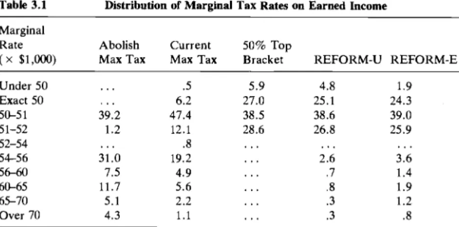
Table 3.1 shows the distribution of marginal tax rates on earned income under the five different sets of tax rules. The percentages shown are of the estimated 2.72 million taxpayers who would have faced marginal tax rates on earned income of 50% or greater had there been no maximum tax. Note that the current maximum tax provision lowers the earned income rate to 50% or less for only 7% of these taxpayers. One-third of these taxpayers have a marginal tax rate on earned income greater than 54%. On the other hand, reducing the top bracket to 50% will lower all marginal rates to under 52%; the same will be accomplished for 95% of these taxpayers by implementing REFORM-U. REFORM-E will lower the tax rate on earned income to 52% or less for 92% of these taxpayers.

The reason that tax rates may be above 50% even if that is the top tax bracket involves some of the income constraints of the tax code. For example, the medical deduction is allowed only for expenses in excess of 3% of adjusted gross income. As earning another dollar will lower deductions by 3 cents, taxable income will rise by $1.03. At a 50% marginal tax rate, the extra dollar earned will increase tax liabilities by 51.5 cents. The marginal tax rates on earned income may be lower than 50% because of the personal income constraint on retirement contributions.

Table 3.2 shows the distribution of the changes in revenue resulting from a change in the maximum tax provision. The current maximum tax rule gives about 60% of the tax reduction to taxpayers with adjusted gross

Table 3.1 Marginal

Rate Abolish Current 50% Top

( x S~,oOo) Max Tax Max Tax Bracket REFORM-U REFORM-E Distribution of Marginal Tax Rates on Earned Income

Under 50 Exact 50 5&5 1 51-52 52-54 54-56 56-60 60-65 65-70 Over 70 39.2 1.2 31.0 7.5 11.7 5.1 4.3 . . . .5 6.2 47.4 12.1 .8 19.2 4.9 5.6 2.2 1.1 5.9 27.0 38.5 28.6 . . . . . . . . . . . . 4.8 25.1 38.6 26.8 2.6 .7 .8 .3 .3 . . . 1.9 24.3 39.0 25.9 3.6 1.4 1.9 1.2 .8 . . .

Note: Percentages reflect the share of 2.72 million taxpayers who would have had marginal tax rates on earned income of 50% or greater if there had been no maximum tax.

(9)

Table 3.2 Distribution of BeneCts/Costs of Tax Changes (number of beneficiarieshosers)

AGI Class Abolish 50% Top

( x $1,000) Max Tax Bracket REFORM-U REFORM-E

Under 50 4,000 53,000 8,000 3,800 50-100 403,000 780,000 729,000 673,000 100-200 349,000 494,000 474,000 407,000 500-1,000 7,000 10,500 10,Ooo 6,500 Over 1,000 1,600 3,400 3,000 1,500 200-500 79,000 105,000 100,000 75 ,000

Average Tax Change

Under 50

+

270 - 90 - 810 - 1,030 50-100

+

440 - 450 - 500 - 470 100-200

+

3,210 - 2,680 -2,030 - 1,800 200-500

+

16,600 - 14,500 - 9,200 - 6,900 500-1,000 +51,700 - 54,300 - 22,000 - 11,Ooo Over 1,OOO

+

151,200 - 246,000 - 46,000 -5,500 Total Tax Change

(millions) Under 50 +1 - 5 - 6 - 4 50-100

+

177 - 351 - 365 -316 100-200

+

1,120 - 1,324 - 962 - 733 200-500

+

1,311 - 1,523 - 920 -518 500-1,000

+

354 - 570 - 220 - 72 Over 1,OOO

+

238 - 836 - 138 - 8

income above $200,000. This compares with 62% for a complete reduction in rates

to

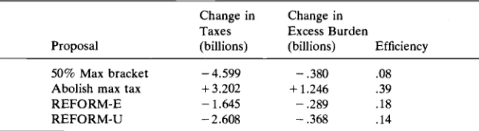
50%, 49% for REFORM-U, and 36% for REFORM-E. Table 3.3 compares the excess burden imposed by different tax regimes. The excess burden measure I use is explained in Yitzhaki (1975). This measure contrasts the taxes actually collected via a labor income tax with what could have been collected via a lump-sum tax and left the taxpayer at the same level of utility. The result takes the familiar form

1 .

2

excess burden = -eiti2U:

,

where ei represents the individual elasticity of labor supply, ti his or her marginal tax rate on earned income, and Wi labor income. The excess burden is an increasing quadratic function of tax revenue collected. If contrasted with the revenue collected, this measure provides a relative efficiency cost of various tax rules. The measure also takes no account of any excess burden placed on capital income. The Wi term reflects only personal service income.

(10)

Table 3.3 Relative Efficiency of Various Tax Changes Change in Change in Taxes Excess Burden

Prop o s a 1 (billions) (billions) Efficiency 50% Max bracket - 4.599 - ,380 .08 Abolish max tax

+

3.202

+

1.246 .39

REFORM-E - 1.645 - .289 .18

REFORM-U - 2.608 - .368 .14

The calculations assume a labor supply elasticity of 0.1 for all indi- viduals. The reader may choose to substitute a different elasticity for this estimate of ei to get a measure of the efficiency of any one tax regime. However, the relative efficiencies of each of the tax changes is unaffected by the choice of elasticity.

As the calculation is a function of the square of the tax rate, a 70% rate will level twice the excess burden of a 50% rate. Abolishing the maximum tax would involve an increase in revenue with twice the efficiency cost of the next highest alternative. REFORM-E involves a reduction in tax revenue of $1.651 billion, but would be the most efficient reduction from the view of the excess burden on labor income. As a reduction to 50% of the top bracket would apply in large part to capital income, the efficiency loss is relatively low.

3.3 Simulation Methods

This paper concentrates on simulating two different kinds of responses by taxpayers to changes in the maximum tax rules: changes in the degree of sacrifice made to work and save, and changes in the avoidance of income tax. Well-established parameter values for these responses do not exist. The taxpayer makes his or her decisions based upon a number of separate yet interrelated margins: work and leisure, savings and consumption, and receipt of taxable income and avoidance of taxable income.

3.3.1 The Effect of Tax Rules on Effort

The effect of a change in tax rules on work effort is the combined result of a substitution or compensated price effect and an income effect. A

reduction in marginal tax rates induces greater effort by raising the after-tax wage. However, the resulting tax reduction increases the taxpayer’s disposable income, producing a countervailing income effect.

Using the Slutsky equation, this may be expressed as

6h 6h

-

=S,,

+

h

-

,

(11)

where h represents labor effort, w the after-tax wage, and y income. The compensated price effect Sw, is constrained to be nonnegative, and ShISy is presumed to be negative.

The labor supply function for individual

i

can be expressed as

where Q represents the uncompensated wage elasticity of labor supply

and

p

the income elasticity of labor supply;

ki

represents the individual’s tastes. The constant elasticity formulation may be defended for changes of the magnitude concerned here, although this specification is not plausible for extreme values.

The Slutsky relation may be expressed in terms of elasticities:

Further manipulation produces an expression in terms of the compensated wage elasticity E,:

wh Y € , = Q - @

- .

The taxpayers subject to the options considered in this paper often have substantial nonlabor income. The compensated elasticity therefore varies substantially across the sample. The quantity whly represents the share of labor income in total income. This has a mean value of roughly 0.75 for current maximum taxpayers.

Nonlabor income affects the labor supply decision by altering the budget constraint between consumption and leisure:

(1 - t ) L

+

M = C

+

(1 - t ) ( L - h )

.

L represents the taxpayer’s endowment and is enumerated in before-tax consumption units. C represents consumption and L

-

h leisure. M is a lump-sum term which includes both capital income and the lump-sum payment implied by the progressive income tax. Hausman (1981) has termed this latter component “virtual income, ”

Figure 3.4 illustrates how a progressive tax system yields a lump-sum term. A worker sacrificing l I hours of leisure works Zo hours tax free and pays a tax

el

on all labor income in excess of lo. The taxpayer’s marginal decision is based on a price of leisure of l - tl but not the full income reduction this would imply if he or she paid tax on the total labor supplied. The taxpayer receives an income transfer of M 1 = elo aside from the tax paid elll. The income transfer M 2 represents

(t2 - cI)(l2 - lo)

+

c 2 4 ;

this is the difference between the tax rate paid on the last unit of labor supplied and the tax rate actually paid on inframarginal units. Note that if the tax rate schedule is known, the income term M

(12)

93 Alternatives to the Current Maximum Tax on Earned Income I

!

I

\

MZ M l -I 42

4

10 Fig. 3.4

is uniquely defined by the taxpayer's last dollar marginal tax rate. Varia- tions of labor supply along any segment, or between any two kinks, do not alter the income term M.

The maximum tax creates a further complication. The marginal tax rates on earned and unearned income are different, and are altered by different amounts in each of the options considered in this paper. The taxpayer faces a consumption-savings choice as well as a consumption- leisure trade-off. The change in the tax rate on capital income might well alter this decision. However, the combined price and income effects of the change produce an ambiguous result on a priori grounds. I assume that aggregate capital income is unaffected by the change in the tax rate on either labor or nonlabor income. However, the reduction in the tax rate on capital income does increase the taxpayer's virtual income. This will tend to depress the supply of labor by the household.

With the exception of abolishing the existing maximum tax, all of the options considered here have a greater effect on the return to capital income than on the return to labor income. The assumption of zero elasticity of capital income to changes in the tax rate is probably an understatement of the response of taxpayers to lower rates and was chosen to minimize predicted revenue changes. Similarly, values which suggest a highly inelastic supply of labor have been chosen for this

(13)

simulation. Four sets of values have been used; the implied compensated elasticity for a typical maximum taxpayer has been computed and is indicated by table 3.4.

Empirical studies of the labor supply of prime age males suggest wage elasticities of zero. The households studied in this paper are overwhelm- ingly married couples and therefore likely to have labor supplies substantially more elastic than this. The parameter values used here imply a labor supply only slightly more elastic than that for prime age males.

3.3.2 The Effect of Tax Avoidance

In the above discussion it was assumed that all income was actually subject to tax. In fact, much income received is not taxed. Tax avoidance may involve donation of income to charitable organizations. It may involve taking advantage of the exclusions available to some forms of capital income. Avoidance also includes tax preferences granted to particular uses of capital or to the purchase of state and local bonds. The tax on much farm, rent, and small business income may be avoided by taking advantage of the separately taxed entity for consumption purposes. A

formal model of all these avoidance decisions is beyond the scope of this paper. It remains a topic of continuing research, however.

For this paper the avoidance decision is approached at the margin. A

utility-maximizing taxpayer would allocate his or her resources in order to equate the marginal after-tax benefits from each purchase. The marginal dollar expended on avoidance brings benefits equal to the marginal dollar less tax used for ordinary consumption purposes. As a result, the price p used above to compute effort is unaffected by the level of tax avoidance. The marginal cost of avoidance also is p .

Because of the maximum tax, taxpayers face different prices for avoiding labor and nonlabor income. The price of some forms of avoidance, in particular preference items, is also increased by the maximum tax. This is due to the “poisoning” provision of the maximum tax law, which treats one dollar of labor income as capital income for each dollar of preference income received. In effect the preferences are taxed at the difference between the unearned income and earned income marginal tax rates, a

Table 3.4 Parameter Values Used in Simulation Implied Wage Income Compensated Elasticity Elasticity Elasticity

0 0 0

0 - .1 .075

,075 - . 1 .15 . 1 - .2 .30

(14)

difference which may be as high as 20%. However, preference income constitutes only a small portion of income which avoids tax. I therefore have taken the price of avoidance as a simple weighted average of the earned ( t e ) and unearned (tu) marginal tax rates, where the weight depends on the share of labor income in total income T:

p = T(1

-

te) + (1 - T)(1 - tu)

.

It is also possible that inframarginal dollars of avoidance cost less than the marginal dollars. This would affect the virtual income of the taxpayer in the same way as the nonlinear tax schedule affected it. A reduction in marginal tax rates would lower the inframarginal income taxpayers re- ceive from low-cost avoidance items and therefore raise labor supply. In order to err on the side of conservatism I have ignored the inframarginal transfer on untaxed income by assuming that all avoidance costs the marginal price.

While the marginal price of avoidance is known, the quantity of income which avoids tax is unknown. I have considered the following relation:

avoidance = A(price, income, tastes)

.

I used a sample of 7,703 returns from the 1977 Individual Tax Model File, the same sample used in the simulations reported in section 3.4. The taxpayer’s total income was estimated as his or her potentially taxable income reported in the file. Potential income was calculated by adding retirement contributions, capital gains deductions, the dividend exclusion, and reported preference income to adjusted gross income. If the taxpayer reported any Schedule E loss, it was excluded. Schedule E gains were unaffected. The standard deduction and personal exemptions for the 1977 tax year were then subtracted as they involve no avoidance behavior by the taxpayer.

Avoidance is calculated as the difference between potentially taxable income and income which is actually taxed. Neither the author nor any reader should consider this a definitive measure. The definition of what should constitute taxable income has concerned such noted economists as Musgrave and Pechman. I do not wish to enter the debate. If anything, this estimate probably understates “true” potential income. Interest from state and local bonds is excluded as are unrealized capital gains, imputed rental income, and the imputed value of household services. NO

effort has been made to estimate tax evasion. On the other hand, some might argue that the inclusion of state and local taxes and charitable contributions is inappropriate. As the taxpayers in this study are liable to have substantial capital assets which are not observed, the relation I estimate probably understates the true effect of price on avoidance.

However, some might argue that much of the estimated avoidance is actually the realization of long-term capital gains. I have therefore de-

(15)

fined an alternative income concept which excludes the capital gains deduction from both the income and the avoidance terms. Four relations were estimated:

(1) RATIOi = CY

+

p

FDARATi

+

ei ,

(2) RATIOi = a

+

p

FDARATi

+

A ln(INCOME)i

+ ei

,

(3) RATIO: =

+

p

FDARATT

+

~i

,

(4) RATIO: = a

+

p

FDARATT

+

A ln(INCOME*)i

+

ei

.

RATIOi is the share of potential income which avoids tax, FDARAT, is the taxpayer’s weighted average of first-dollar tax rates on earned and unearned income, and INCOMEi is the taxpayer’s potential income. The asterisk denotes the alternative concept of avoidance, which excludes the capital gains deduction. A first-dollar rate was used to minimize possible simultaneity problems. That is, the rate used was the rate which would have applied had the taxpayer avoided tax on only one dollar of income. There seems no a priori reason why the share of income which avoids tax should vary systematically with income. Inclusion of an income term in equations (2) and

(4)

is done to test for possible scale economies in avoidance or for the possibility that, aside from the higher marginal tax rates, tax avoidance behavior is associated with being rich. The results suggest that income is not an important factor:

(1) RATIO = - 0.086

+

0.742 FDARAT , (0.006) (0.012) (0.009) (0.026) (0.00 16) (0.006) (0.011) (0.009) (0.024) (0.001 5 ) RATIO = - 0.084

+

0.748 FDARAT (2) - 0.0004 ln(INC0ME) , (3) RATIO* = - 0.074

+

0.686 FDARAT* , RATIO* = - 0.067

+

0.708 FDARAT* (4) - 0.0016 ln(INC0ME)

.

Standard errors are reported below the coefficient. The income coefficient is both small and insignificant. The price term has a highly significant t statistic, and all four equations are significant to the 0.9999 level using an F test. The R-square terms range from 0.329 to 0.341, which is quite reasonable for cross-section data. The exclusion of long-term capital gains deductions has little effect on the coefficient.

(16)

The usual collinearity of income and the tax rate is substantially reduced by the maximum tax. Taxpayers earning from $60,000 to $10 million may have marginal tax rates of 50%, while taxpayers within this range may have rates as high as 70%. In fact, the marginal tax rate on earned income falls as earned income rises for maximum taxpayers and the rate on unearned income may also fall as unearned income rises (see Lindsey 1981). The maximum tax provision therefore permits substantial enough variation between rate and income to make estimation possible.

This estimated response of taxpayers to changes in marginal tax rates suggests that 0.7% less income will avoid tax for each 1% reduction in the marginal tax rate. This paper also presents estimates using a simulated response only half as great; that is, an additional 0.35% of potential income is subject to tax for each 1% reduction in the tax rate.

As an example of this effect, consider a married couple with potential income of $100,000 of which $20,000 is capital income. Their current avoidance price is 44 cents on the dollar (an average marginal tax rate on earned and unearned income of 56%). They avoid taxes on roughly 31% of their income. A tax rate reduction to 50% would mean an increase in their taxable income of $4,200, from $69,000 to $73,200. This is certainly a plausible order of magnitude. The actual simulation procedure uses the taxpayer’s actual ratio of taxable income to potential income and adjusts the ratio by the avoidance parameter value times the change in the marginal tax rate.

3.3.3 Combining Behavioral Effects

This behavioral model assumes the taxpayer responds simultaneously to prices on two margins. The share of the taxpayer’s income which avoids tax is determined by a first-dollar price based upon his or her potential income. The amount of potential income is determined by a constant elasticity type of response of labor income to the last-dollar tax rate on earned income and its corresponding virtual income. But these terms are determined by the share of potential income which avoids tax.

The simultaneous optimization of potential income and share which avoids tax is computed in the following manner: first, the taxpayer’s current first- and last-dollar prices are computed by TAXSIM. Then the first- and last-dollar prices are computed given the alternative set of maximum tax rules assuming no behavioral response by the taxpayer. The difference between the first-dollar prices under current law and the alternative law is used to compute a new percentage of potential income which avoids tax.

This new percentage of avoidance is applied to an unchanged level of potential income to generate a measure of taxable income assuming only the avoidance response. This measure of taxable income is equivalent to

(17)

assuming that the taxpayer has a zero price and income elasticity of labor supply. Marginal tax rates on earned and unearned income are computed given this new level of taxable income. If these tax rates are the same as the tax rates under current law, no increase in labor supply can be expected. If these new tax rates are different from current law, a new level of virtual income is computed and a new level of effort results. This new level of effort or potential income may lead to a new level of avoidance if the higher potential income produces a new first-dollar tax rate. If not, the old level of avoidance is retained.

The new avoidance measure is used with the new potential income to produce a new level of taxable income. If the marginal tax rates at this level of taxable income equal the earlier tax rates, a stable preference decision has been reached. If not, the iteration procedure continues until the new set of tax rates equals an old set of tax rates.

A possible problem with this iterative procedure is the kinked nature of the budget set. Iteration may produce a result alternatively at a high and a low price. Figure 3.5 shows such a possibility. The true utility-maximizing value for the taxpayer is to be on the kink. But the iterative procedure evaluated at p1 will place the taxpayer at l2 on the p 2 segment, and evaluation at p 2 will place the taxpayer at

ZI

on the p1 segment. If this result occurs, the kink between the two segments is automatically chosen. The price and virtual income corresponding to the higher segment, in effect a “next”-dollar price, is used for evaluation.

3.3.4 Simulation Procedure Differences among the Options

The two relevant prices, one applying to extra sacrifice, the other to avoidance behavior, depend upon the option considered. For example, the abolition of the maximum tax, or the alternative option of cutting the maximum statutory rate to 50%, involves equal tax rates on earned and capital income. On the other hand, the existing maximum tax and the two reform options may involve different marginal tax rates on earned and unearned income. For these latter two options a weighted average of the earned and unearned tax rates is used to estimate the last-dollar price.

The first-dollar price, the price of avoidance, is different for the two reform options than for the former options mentioned. If all deductions are applied to earned income, then the price of avoiding a dollar of taxable income is determined by the earned income tax rate. If the deductions are applied to unearned income, then the price is determined by the unearned income tax rate. The present price of avoidance is a weighted average of the first-dollar earned and unearned tax rates.

If deductions are applied to unearned income, then some taxpayers may see a decrease in the price of avoidance. This will lower the share of income which is reported and reduce tax revenue. If, on the other hand, deductions are applied to earned income, an unambiguous increase in the

(18)

99 Alternatives to the Current Maximum Tax on Earned Income

-4

Fig. 3.5

price of avoidance will result. This will lower the share of potential income which avoids tax and will tend to produce higher revenues.

Lowering the maximum rate to 50% on all income also unambiguously increases the price of avoidance, thereby increasing taxable income. On the other hand, increases in avoidance will occur among taxpayers currently benefiting from the maximum tax if it is abolished. The next section examines the effect of these behavioral changes on income tax revenues.

3.4 Results

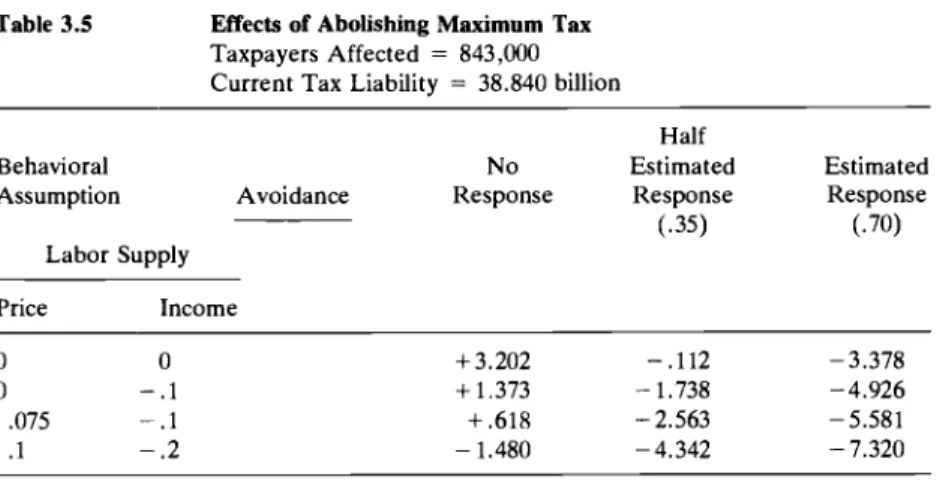
The results of the simulations are presented in tables 3.5-3.8. The surprising conclusion one can draw is that it is possible to reduce marginal tax rates and still increase tax revenue. Table 3.5 suggests that the existing maximum tax provisions are probably a revenue raiser in that abolishing the maximum tax will lead to a decrease in tax revenue. Even at half the estimated value of the avoidance response, tax revenues are simulated as decreasing when the rates are increased. Table 3.5 gives the best picture of a labor supply response, as the current maximum tax

(19)

Table 3.5 Effects of Abolishing Maximum Tax Taxpayers Affected = 843,000 Current Tax Liability = 38.840 billion

Half

Behavioral N o Estimated Estimated

Assumption Avoidance Response Response Response

(.35) (.70) Labor Supply Price Income 0 0 0 - .1 ,075 - . 1 .1 - .2 +3.202 -.112 -3.378

+

1.373 - 1.738 -4.926

+

,618 - 2.563 -5.581 - 1.480 - 4.342 -7.320

yielded a reduction in the marginal tax rate on earned income far greater than any of the other options considered. The greatest response simulated yielded $4.7 billion more in tax revenue from the labor supply effect alone while even the most modest labor supply response yielded nearly $2

billion more in revenue than the no-response case.

Even in this case the avoidance response is likely to dominate the labor supply response. If no labor supply response is assumed, $6.6 billion more in revenues is raised due to less avoidance. The avoidance response is not the usual “supply side” response commonly discussed today. No additional factors of production are brought forth. Rather it reflects a transfer of resources from favored activities to the taxpayer and the government. The actual welfare change is ambiguous.

Table 3.6 shows that a further reduction of tax rates to a statutory limit of 50% will be a revenue raiser if the full avoidance response occurs. The labor supply response is relatively small. In the no-avoidance case an

Table 3.6 Effects of Establishing a Maximum Bracket Taxpayers Affected = 1,446,000

Current Tax Liability = 59.369 billion Half

Behavioral No Estimated Estimated

(.35) (.70) Labor Supply Price Income 0 0 -4.559 - 1.338

+

1.817 0 - .1 -4.500 - 1.285

+

1.944 ,075 - .1 - 4.225 - .988

+

2.225 .1 - .2 -3.995 - .827 i 2 . 4 7 4

(20)

101 Alternatives to the C u r r e n t Maximum T a x on Earned Income

Table 3.7 Effects of Applying Deductions to Unearned Income Taxpayers Affected = 1,323,OOO

Current Tax Liability = 59.447 billion Half

(.35) (.70) Labor Supply Price Income 0 0 - 2.608 - 2.246 - 1.856 0 - . 1 -2.546 -2.228 - 1.783 ,075 - .1 -2.289 - 1.991 - 1.538 .1 - .2 -2.099 - 1.867 - 1.357

additional $600 million may be raised, or $1.2 billion additional earned. The reduction in the top rate to 50% will largely affect nonlabor income. A negative income effect on labor supply will therefore substantially offset the extra effort produced by the reduction in the earned income rate. If a capital income response is also included, an additional revenue increase of roughly one-third the order of magnitude of the current maximum tax will result. The revenue cost of a 50% maximum rate is therefore overstated by this simulation by $1 to $2 billion if one assumes that capital income will respond like labor income.

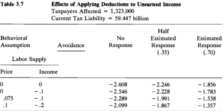
Applying deductions to unearned income is likely to be a revenue loser. As the unearned tax rate may well be higher than the current average of earned and unearned rates, avoidance may well be even more attractive under this reform for many taxpayers. Even the maximum avoidance response will produce only $750 million as a revenue offset. Applying deductions to earned income has two benefits from a revenue Table 3.8 Effects of Applying Deductions to Earned Income

Taxpayers Affected = 1,168,000

Current Tax Liability = 47.596 billion Half

(.35) (.70) Labor Supply Price Income 0 0 - 1.645 - ,070

+

1.399 0 - .1 - 1.552 - ,023

+

1.499 .075 - .1 - 1.340

+

,193

+

1.730 .1 - .2 - 1.145

+

.309

+

1.941

(21)

point of view. First, it is a less costly option even assuming no response. This is because current avoidance partially offsets nonlabor income under current rules. Under this option avoidance would reduce the tax liability by only the earned income marginal rate. Second, the behavioral response to avoidance would be greatest, as the price of avoidance has been increased to 50 cents on the dollar. This will mean that a higher fraction of income will be subject to tax.

In conclusion, it is likely that a reduction or reform of the upper brackets of the tax rate schedule would be relatively costless or might even increase tax revenues. However, a majority of the revenue offset from a behavioral response does not come from an increase in factor supply. Rather it is a pecuniary gain to the government and taxpayers as a result of less expenditure on tax avoidance. The high labor supply elasticities used in many supply side models of the economy may exaggerate the benefits of a tax rate reduction. However, the neglect of the avoidance response by any model produces a serious overestimate of the revenue cost of marginal rate reductions.

References

Auerbach, A. J., and H.

S.

Rosen. 1980. Will the real excess burden please stand up? NBER Working Paper no. 495. June.

Burtless, G., and J. Hausman. 1978. The effect of taxation on labor supply: Evaluating the Gary negative income tax experiment. Journal of Political Economy, vol. 86, no. 6.

Fullerton, D. 1980. On the possibility of an inverse relationship between tax rates and government revenues. NBER Working Paper no. 467. April.

Hausman, J. 1981. Labor supply. How taxes affect economic behavior.

Washington: Brookings Institution.

Kahn, H. 1960. Personal deductions in federal income tax. NBER Fiscal Studies, no. 6. Princeton, New Jersey: Princeton University Press. Lindsey, L. 1981. Is the maximum tax on earned income effective?

National Tax Journal, June.

Yitzhaki. 1975. Personal taxation incentives and tax reform. Mimeo, University of Jerusalem, Israel.

(22)

103 Alternatives to the Current Maximum Tax on Earned Income

Comment

Joseph J. Minarik

The first part of Lindsey’s paper, dealing with marginal tax rates on earned income of over 50%, is not controversial. This basic finding was stated in 1974 by Emil M. Sunley, Jr., in his paper “The Maximum Tax on Earned Income” (National Tax Journal 27: 543-52, especially 545+6), which is not cited in Lindsey’s paper.

There are also no basic problems with the second part of the paper, the static revenue estimates. Lindsey’s results are in close agreement with similar tabulations using the Brookings tax calculator. There are, however, two points of interpretation that should be discussed.

Lindsey correctly states that there are over 2.5 million taxpayers who would be subject to marginal tax rates on earned income of over 50% at 1981 income levels and without the current law’s maximum tax provision in place. What Lindsey noted in an earlier draft of the paper but (in my view unfortunately) omitted from the conference version is that this group is quite heterogeneous. In fact, it can be subdivided into three distinct parts. First, there are those taxpayers who are categorically ineligible to use the maximum tax because they use income averaging or file separate returns. These taxpayers constitute 36% of the larger group. The second category includes those taxpayers with too little earned income to qualify for the maximum tax under the present stacking rules; in other words, their earned income alone is not enough to reach beyond the 50% tax bracket. This category includes 34% of the larger group. The remainder of the roughly 2.5 million taxpayers use the maximum tax provision.

My understanding is that Lindsey’s proposed changes to the maximum tax provision would not remove the categorical restrictions on its use. However, taxpayers who have insufficient earned income to qualify under current law would be provided substantial tax relief: $0.6 billion if deductions were applied to earned income. Only $1.1 billion of the total static revenue losses would accrue to those currently using the maximum tax provision. When the maximum tax was suggested in 1969, the House was very conscious of revenue constraints and sought to target the provision as carefully as possible (House Ways and Means Report, pp. 208-9). The Senate deleted the provision, again largely for revenue reasons (Senate Finance Report, pp. 309-10). The revenue loss question is at least as important now as it was in 1969, and targeting is again relevant. The Brookings tax calculator projected that the category of returns with Joseph J . Minarik is a research associate in the Economic Studies Program, the Brook- ings Institution, Washington.

Tim Cohn and Ed Shephard provided their usual stellar research assistance. Susan Woollen typed the manuscript against all odds; any errors that appear are the author’s. Research funds were provided by the National Science Foundation.

(23)

too little earned income to qualify for the current maximum tax provision would average only $22,000 of earned income per return in 1981; this group is composed substantially of investors and rentiers whose labor income is a distinctly secondary source of support. Whether their labor supply is at all elastic to wage rates is, at least in my opinion, highly questionable; and the deadweight revenue loss (and thus the counteract- ing income effect) of their inframarginal labor supply is clearly substantial.

A second question of interpretation is the relative success of the current maximum tax provision in reducing marginal tax rates. To phrase Lindsey’s verbal evaluation just a bit differently, the current provision reduces the marginal tax rate on earned income to 52% or less for 66% of those now facing rates over 50%; his earned and unearned deduction allocation regimes achieve 52% rates or lower for 92 and 95% of the taxpayers, respectively. The margin of performance may not be as great as a first reading of the paper would suggest. And, of course, part of the reduction in rates that Lindsey’s changes achieve is due only to the inclusion of taxpayers with low earned income who are ineligible under current law. If we restrict our view to those currently using the maximum tax provision, 77% achieve rates of 52% or lower under current law, more than the 66% for the entire universe. Here again, a substantial portion of the effect of Lindsey’s law changes relates not to the problems with the current code, which he did discuss, but rather to the inclusion or exclusion of particular taxpayers within the current provision, which he did not discuss.

This leaves for discussion only the behavioral revenue estimates. The most important question is how Lindsey arrives at his surprising finding that liberalizing the maximum tax provision will raise revenue.

Lindsey’s labor supply responses are based on a simple application of wage and income elasticities chosen to represent the range of estimates in the literature. My own judgment is that the compensated wage elasticities of 0.0 and 0.075 are quite adequate to bracket the feasible range, even though Lindsey presents two larger response estimates. My pessimism is based partly on the likely inelasticity of the labor supply in hours of individual high-wage workers, who probably already work full time and bear considerable responsibility in their present jobs. Another cause for skepticism is that Lindsey is implicitly using in the simulations not a wage rate elasticity of hours worked but a wage rate elasticity of earnings. It seems by no means certain that additional hours of effort will command the same wage as the inframarginal hours, especially for the married couples on whom Lindsey so heavily hangs his hat. For an extreme example, one might concede that a 30% reduction in the marginal tax rate on earnings might induce the heretofore idle spouse of the chief executive officer of a major corporation to increase the family’s hours

(24)

worked by

lo%,

but one would be hard pressed to imagine that he or she could find work at the spouse’s hourly wage rate.

Nevertheless, the labor supply response is a largely academic issue, because it accounts for only a small fraction of the projected revenue response-about $500 million at the very outside, or more likely only about $100 million, of the static revenue losses of about $1.5 and $2.5 billion due to the proposed liberalizations of the maximum tax. Thus the real revenue raiser is the anticipated response of reduced “tax avoidance,” the most speculative part of Lindsey’s work.

It seems to me unlikely that the stronger taxpayer response to a cut in taxes on earned income will come through reduced tax avoidance rather than greater earnings. On careful consideration, I must conclude that Lindsey’s estimates of reduced tax avoidance are extremely shaky and represent overstatements of the likely effects.

The most basic problem with Lindsey’s estimates of tax avoidance behavior is his measure of tax avoidance itself. He defines avoidance as the difference between taxable income and “potential taxable income,” which is equal to the sum of adjusted gross income and a list of additional items: the excluded portion of long-term capital gains, retirement contributions, the dividend exclusion, reported preference income, and Schedule E losses. This definition is replete with problems. Are state and local tax liabilities “avoidance”? Are medical expenses? Casualty losses? Implicitly, Lindsey is assuming that a reduction in the marginal tax rate on earned income will cause an increase in taxable income equal to a proportion of this potential income concept, which includes (at least in my opinion) many income items that are quite irrelevant for this purpose. Nor is Lindsey’s disclaimer that the “definition of what should constitute taxable income has concerned

. . .

noted economists

. .

.

I do not wish to enter the debate” in any way satisfactory. After Lindsey has fitted regression equations to his concept of potential taxable income and projected that proportions of it will be added to actual taxable income, given his proposed changes in the tax law, he cannot avoid the debate. He has dived into it headfirst, like it or not.

Finally, Lindsey’s assertion that “[if] anything this estimate probably understates true ‘potential”’ is no comfort whatsoever. If the measure of potential income is conceptually wrong, be it too high or too low, then its correlation with tax rates yields no information on true tax avoidance behavior.

The second major problem with Lindsey’s measure of tax avoidance behavior is his estimation procedure. He fits a very simple linear regression equation to data on tax rates and the ratio of taxable income to his potential income, and finds a positive correlation between tax rates and his concept of tax avoidance. This procedure can be faulted on several counts. First and most fundamentally, if the concept of potential income

(25)

is not a good representation of tax avoidance behavior, as was suggested above, then the entire exercise is irrelevant.

But even if the present concept of tax avoidance is accepted, the model seems much too simplistic to capture anything approaching the full complexity of taxpayer behavior with respect to the items added into Lindsey’s potential income. Such important and omitted variables as the taxpayers’ ages, wealth, split of income between property and labor sources, etc., surely render the equation a victim of misspecification.

Lindsey’s inclusion of a potential income variable in two of his equations does not solve this specification problem. For much the same reason as was mentioned above, if the potential income concept has no meaning in this context

,

adding a potential income variable to the equation cannot make it meaningful.

Lindsey cites the similarity of the tax rate coefficients in the two versions of his equation, one including and one not including the capital gains exclusion as a tax avoidance item, as an indication that his estimates are sound. At least in my opinion, that similarity is the best indication that his estimates are not well founded. Figure C3.1 shows that the capital gains exclusion accounts for a large share of what Lindsey originally defined as tax avoidance and that the share increases rapidly as income increases. It is hard to understand how the share of potential income that avoids tax could remain almost the same when such a large part of tax avoidance is defined out of the game. To see this, consider Lindsey’s results from the equation that does not cover the excluded half (using 1977 law) of long-term gains. Suppose that the top bracket rate were reduced from 70 to 50%. Then, using Lindsey’s coefficient, the 78.5% of all taxpayers with adjusted gross income of $500,000 and up who now face a 70% top rate (exclusive of the maximum tax) would reduce their tax avoidance according to Lindsey’s definition by 49%-which is equivalent to totally suspending the use of all tax preferences under the minimum tax, forswearing all net losses on Schedule E, not claiming the dividend exclusion, making no tax exempt retirement contributions, and giving up half of all itemized deductions exclusive of state and local taxes paid. This seems an unreasonable result to me.

In any event, even though the coefficients of the two versions of the equations are virtually the same, the tax avoidance behavior will be drastically different depending on whether the capital gains exclusion is included in or excluded from the tax avoidance base. Unfortunately, Lindsey never tells us whether his simulations include or exclude a capital gains tax avoidance effect.

Summary

Lindsey’s assessment of marginal tax rates under the maximum tax is well founded and agrees with a discussion of the subject published much

(26)

Percent of Potential Income

$50,000- $1 00,000 $1 00,000- $200,000 $200,000- $500,000 $500,000- $1,000,000

Adjusted Gross Income

Other Tax Preferences Excluded Capital Gains

Dividend Exclusion 8 Schedule E Losses Retirement Contributions

Excess Itemized Deductions Taxable Income

Over $1,000,000

(27)

earlier. His measures of the static revenue loss from modifications to the maximum tax to hold marginal rates closer to 50% are reasonable. His estimates of the range of revenue recovery due to greater labor supply probably exaggerate the actual response somewhat, especially because of the use of numbers approximating the elasticity of the supply of hours for what is in the simulation really an elasticity of earnings. However, Lind- sey’s middle-range parameters probably show something like the true supply response, and it is quite small.

It is in a “tax avoidance” response that Lindsey finds the jet propulsion for his revenue-raising simulations. He downplays his definition of tax avoidance, saying he “[does] not wish to enter the debate,” but then goes on to use his definition to simulate a behavioral response anyway. In my view the definition of tax avoidance is faulty, the estimates of behavioral responses are too simplistic to embrace the complexity of taxpayer behavior, and the forecasts are unrealistic. Until we learn a lot more about tax avoidance behavior than we now know, Lindsey’s claim that “it is likely that a reduction or reform of the upper brackets of the tax rate schedule would be relatively costless or might even increase tax revenues” must be considered an assertion, not a demonstrated fact.