Multivariate Short term Traffic Flow Forecasting Using Time Series Analysis

MULTIVARIATE SHORT-TERM TRAFFIC FLOW

FORECASTING USING TIME-SERIES ANALYSIS

Bidisha Ghosh, Biswajit Basu, and Margaret O’Mahony

Department of Civil, Structural and Environmental Engineering

Trinity College, Dublin

ABSTRACT: (156 words)

The existing time series models used for short-term traffic condition forecasting are

mostly univariate in nature. Generally the extension of the existing univariate

time-series models to a multivariate regime involves huge computational complexities. A

different class of time-series model called structural time-series model (STM) (in its

multivariate form) has been introduced in this paper to develop a parsimonious and

computationally simple multivariate short-term traffic condition forecasting

algorithm. The different components of a time-series dataset such as the trend,

seasonal, cyclical and calendar variations can be modelled separately in STM

methodology. A case study in Dublin city centre with serious congestion is performed

to test the effectiveness of the forecasting strategy. The results indicate that the

proposed forecasting algorithm is an effective approach to predict the real-time traffic

flow at multiple junctions within an urban transport network where the junctions are

INTRODUCTION

Implementation of Intelligent Transportation Systems (ITS) to provide dynamic

traffic control requires continuous forecasting of traffic conditions in near (short-term

or less than 1 hour, (Smith et al., 2002)) future. Short-term traffic forecasting is an

important tool to follow evolution of traffic conditions over time in a transport

network. This type of advanced forecasting methodologies having a time horizon of

15 minute or less (Smith et al., 2002) can provide information to support short-range

operational modifications to improve the efficiency of the network at a finer scale.

With the increasing need to develop more adaptive (site and time specific) traffic

management systems, considerable research attention has been focussed on short-term

traffic forecasting.

The well-known short-term forecasting algorithms can broadly be classified into

univariate and multivariate approaches. The univariate approach is based on

modelling traffic condition related variables (such as speed, flow or occupancy etc.)

utilising observations from any single site, whereas developing a single model

considering several sites for input and output is termed a multivariate approach.

Unlike univariate models, these models are capable of capturing the temporal as well

as the spatial evolution of traffic conditions over time in a transportation network.

But due to ease of computation, univariate models are more common in short-term

traffic forecasting literature (Kamarianakis and Prastacos, 2003).

Both multivariate and univariate models can be developed using different empirical

(non-parametric and (non-parametric) employ a fairly standard statistical methodology and/or a

heuristic method for traffic flow forecasting without referring to the actual traffic

dynamics. The non-parametric techniques include non-parametric regressions (e.g.

Davis and Nihan, 1991) and neural networks (e.g. Smith and Demetsky, 1994;

Vlahogianni et al., 2005). Due to an intrinsic multi-input nature neural network

models are often favoured in the space-time or multivariate models (Zhang et al.,

1998). The parametric techniques include different time-series models such as, linear

and non-linear regression, historical average algorithms (e.g. Smith and Demetsky,

1997), smoothing techniques (e.g. Smith and Demetsky, 1997; Williams et al., 1998)

and autoregressive linear processes (Ahmed and Cook, 1979; Levin and Tsao, 1980;

Hamed et al., 1995; Williams et al., 1998; Williams, 2003). Of all autoregressive

linear processes, seasonal auto regressive integrated moving average (SARIMA)

models (e.g. Williams et al., 2003 and Ghosh et al., 2005) perform better than other

time-series techniques (Chung and Rosalion, 2001; Smith et al. 2002).

With a few exceptions (Whittaker et al., 1997; Kamarianakis and Prastacos, 2002;

Williams, 2003; Kamarianakis and Prastacos, 2003) most of the literature in

short-term traffic forecasting focus on univariate. The available multivariate empirical

models in the short-term traffic forecasting literature are mainly multivariate

variations on the existing univariate parametric statistical models, e.g. the multivariate

ARIMA model (Kamarianakis and Prastacos, 2003), space-time ARIMA model

(Kamarianakis and Prastacos, 2002). These models can account for the dimension of

space in a transport network. But the models are computationally demanding as the

time-series models based on state-space methodology were introduced as a short-term

traffic forecasting technique by Stathopoulos and Karlaftis (2003).

In this paper, for the first time in traffic flow related studies, multivariate structural

time-series (MST) models are applied to model traffic flow observations from

multiple intersections within an urban signalized transport network. In a structural

time-series model (STM), the evolution of different components of time-series data

such as the trend, seasonal, cyclical and calendar variations with time can be modelled

separately. Classical time-series analysis using the ARMA (SARIMA, ARIMAX)

class of models is based on the theory of stationary stochastic processes. Hence the

time-series dataset to be modelled using the SARIMA technique is always required to

be checked for its stationarity. If the dataset is not stationary, then transformations are

required to be performed to achieve weak stationarity. As STM is not based on this

theory, no such transformations or checks are required for the application of this

methodology. The MST models are computationally inexpensive as compared to

other multivariate time-series models. Missing observations and inclusion of

exogenous variables like traffic flow observations of other upstream junctions can be

incorporated comparatively easily in the MST model (Harvey, 1989; West and

Harrison, 1997; Durbin and Koopman, 2001).

THEORETICAL BACKGROUND

The STM methodology is a particular time-series analysis technique which is set up in

terms of components which have a direct physical interpretation (Harvey, 1989). The

cyclical and calendar variation together with the effect of explanatory variables and

interventions (outlier and structural breaks). The basic principle behind a STM is

similar to that of the Holt Winters Exponential Smoothing (HWES) model, but more

complex. Multivariate STMs are straightforward extension of the univariate STMs

and involve less computational complexities than the other existing multivariate

time-series techniques. An overview of the univariate and multivariate STM model

definitions is given in this section. A detailed discussion on this subject is available in

Harvey (1989) and Durbin and Koopman (2001). A software package called STAMP

6.0 (Structural Time-Series Analyser, Modeller and Predictor) is used in this study for

modelling traffic flow observations using STM.

Univariate STM Methodology

A univariate structural time-series model is formulated based on the unobserved

components which have a direct interpretation in terms of the temporal variability of a

time series dataset. Consequently the evolution of the components such as trend or

seasonality over time and their contribution to the final predictions can be observed

clearly. A univariate STM for a time series dataset y can be described by the

following general equation involving all possible types of temporal components in its

form:

2

,

NID (0, )

t t t t t t

t y                  

where, t is the trend, t is the seasonal, t is the cycle, t is the first-order AR

component and _t is the irregular or the random error. For the purpose of traffic flow

modelling, the univariate and multivariate STM are considered to be comprised of

three components; stochastic trend, seasonality and irregular. Hence, the equation 1

reduces to the following form:

2

,

NID (0, )

t t t t

t y               (2)

The stochastic trend component (_t) represents the long-term movement in a

time-series which can be extrapolated into the future. In the case of traffic flow

observations over a few weeks from a developed urban transport network, this

long-term movement does not show any significant gradient and should be modelled for

the local fluctuations. A Markov model of the stochastic trend can be considered in

this purpose.

1

2

NID (0, )

t t t

t              

(Change of slope is not considered) (3)

The irregular disturbance/variance_2 and the stochastic trend (level) variance_2 are

mutually uncorrelated. The t process collapses to a linear trend if 2

0



  . The

trigonometric specification of the seasonal component as this ensures smooth changes

in the seasonal as observed in traffic flow time-series data.

[ / 2] , 1

s

t j t

j

 







,

, , 1 ,

* * *

, , 1 ,

where each is generated by

cos sin 1,...,

2

, ,

sin cos _{1,..., ,}

j t

j t j j j t j t

j t j j j t j t

s j t T           _              _              (5)

Where, _j 2 j

s



  is the frequency, in radians, and the seasonal disturbances

* and

t t

  are mutually uncorrelated random normal disturbances with zero mean and

common variance _2. When s is even, the equation 5 at

2 s

j collapses to

, cos , 1 ,

j t j j t j t

    _  (6)

Equations 1 to 5 define the STM used in this study. The disturbances of the individual

components of the STM (_2,_2 and_2) mentioned in these equations are all

mutually uncorrelated. The variances _2,_2 and_2 denote the extent to which the

individual components, such as the trend or seasonal component will vary with time

The equations 1 to 5 are generally solved in state-space form using Kalman filter

based algorithms (Kalman, 1960; Harvey, 1989). The hyperparameters and the

components are estimated using maximum likelihood estimation method.

In some cases, the time series observations to be modelled have dynamic relationships

with some other independent variables. They are called explanatory or exogenous

variables and inclusion of these variables in STM, may improve the forecasting

precision of the models. The inclusions of the explanatory variables change the first

part of equation 1 to the following form:

, 1 0

q k

t t t t t i i t t

i

y _x _



    _ 

 

    



where, x_{i t, } is an exogenous variable, k is the total number of exogenous variables,

is the time lag and _i is a set of unknown constants. The significance of is that

in some cases, the lagged value of the dependent variable can be considered as an

exogenous variable in STM.

Multivariate STM Methodology

Multivariate time-series data can be chiefly classified into two distinct types, Panel

data and interactive data (Harvey, 1989). In the case of panel data, the time-series

variables are subjected to the same or similar influences but the individual elements

do not interact with each other. As the variables follow a similar temporal nature, they

of a set of variables which have some behavioural relationships among themselves

and interact dynamically with each other. This distinction is important to find out the

suitable type of multivariate structural time-series analysis technique. The

multivariate traffic flow observations (i.e. observations from different stations in the

same transport network) modelled in this paper are considered to be subjected to

similar influences but not to have any dynamic interaction (detailed explanation in

next section) and are modelled as panel data.

The panel data can be modelled by a multivariate structural time-series (MST)

technique where the various components of the different time-series variables are

allowed to be contemporaneously correlated. Such a type of MST model is referred to

as, seemingly unrelated time-series equations (SUTSE) (Harvey, 1989). The

univariate equations described in the previous subsections can easily be extended to

SUTSE model.

,

NID (0, )

t t t t

t         

y   

 

t = 1,…., T (8)

where, y_t is a vector of N1time-series observations which depends on the

unobserved trend component , _t seasonal component _t and irregular component _t

which are also vectors. _ is the NN variance matrix of the irregular disturbances.

In multivariate regime, the equations 3, 4, 5 and 6 change in a similar manner as in the

become vectors in the MST model and the disturbances of these components become

NN variance matrices.

The inclusion of explanatory variables in the MST model is simple and similar to the

univariate approach described in equation 7.

0

q

t t t  t  t

 

  



y    x  (9)

where, x_t is a vector of K1explanatory variables. Elements of the unknown

parameter matrix _ can be specified to be zero, thereby excluding certain

explanatory variables from particular equations.

A vector process y_t is said to be homogenous if all linear combinations of its N

elements have the same stochastic properties. In a multivariate homogenous system,

the disturbance matrices are required to satisfy the following equation:

*

*

and

k qk

h 





 

 

(10)

where, q_k, k = 1,……, g and h are non-negative scalars and _* is an NN matrix.

In these ?? cases possible assumption of homogeneity in a SUTSE model decreases

One of the major advantages of STM methodology is its transparency (Durbin and

Koopman, 2001). In STM, the different components which make up the time-series

are modelled separately unlike the SARIMA methodology (e.g. Williams and Hoel,

2003 and Ghosh et al., 2005) where the trend and seasonal components are eliminated

by differencing. Hence, in STM it is easy to understand the evolution and contribution

of each of the components in the final results. In a multivariate regime, MST models

are straightforward vector extensions of the univariate STM. The SUTSE models do

not involve estimation of huge co-variance matrices as Vector ARMA (VARMA)

models. Due to the recursive nature of the STM models any known structural change

over time is easy to implement, whereas SARIMA models cannot include such

structural changes since they are homogenous and stationary in form. Treatment for

missing values in a time-series is also very simple in STM equations. Explanatory

variables, outliers, structural breaks etc. can also be easily modelled in a STM

framework as described before. Introduction of the same variables in SARIMA

models require tedious computational efforts. STM is more general, flexible and can

be easily transferred from a univariate to multivariate regime than the ARIMA class

of models.

METHODOLOGY

A multi-input multi-output (where the number of input intersections are more than

number of output intersections) short-term traffic flow simulation and forecasting

model is proposed in this study for efficient modelling of traffic in a congested urban

traffic volume observations from different approaches and different intersections of

the transport network.

Unlike the previous multivariate traffic flow models developed for urban transport

networks (Stathopoulos and Karlaftis, 2003; Kamarianakis and Prastacos, 2002), the

locations of the sites of data collection within the transport network are not required to

be considered in the proposed methodology. The aim of this approach is to develop a

multivariate traffic flow simulation and forecasting model for multiple intersections

within a transport network which may not be situated on the same route. As the

intersections or stations of observations are not situated on the same route it is highly

unlikely that the same platoon of vehicles will pass through different intersections at

different time instants. Hence, information about the directions of traffic flow is not

essential. A SUTSE model is ideal for modelling such multivariate time-series

observations as the behavioural relationship among the variables are not considered.

As an improvement to the panel data modelling methodology a spatial dimension is

introduced to the proposed multivariate traffic flow model. The traffic flow

observations from the nearest available upstream intersection of each of the modelled

data collection stations are included as explanatory variables to the MST model

equations. This ensures that the effect of any abrupt change occurring in the upstream

junction can be accounted for in the model.

APPLICATION OF THE PROPOSED MST MODEL

The proposed multivariate traffic flow forecasting methodology is applied to a

congested urban transportation network in the city centre of Dublin to test the

effectiveness of the forecasting strategy. A small network of ten intersections within

the transport network is chosen for this purpose.

The time interval of traffic flow observation data collection is unique to the data

collection system of the existing urban traffic control system of any city. The data

interval can vary from a few seconds to one hour. Short-term forecasting algorithms

applicable to a traffic management system should have a prediction horizon of 15

minutes or less (Smith and Demetsky, 1997). The univariate traffic flow observations

obtained over each 15 minute interval from the inductive loop-detectors situated at

these ten intersections and their nearest available upstream junctions are modelled

using the proposed multivariate traffic flow model. There are two important points

which are required to be checked before applying the proposed methodology.

1. The location and the distance of the sites can be chosen at random. The only

criteria for the choice is that the average travel time between two sites on the

same route within the network should not be more than 15 minutes.

Considering a 30 km/hr free flow speed within a congested urban transport

network, the radius of the simulation network should not be more than 7.5

km.

2. The second and the most important point is that the univariate traffic flow

observations from different data-collection sites should not have behavioural

multivariate traffic flow observations behave as a panel data set, the SUTSE

model can be applied.

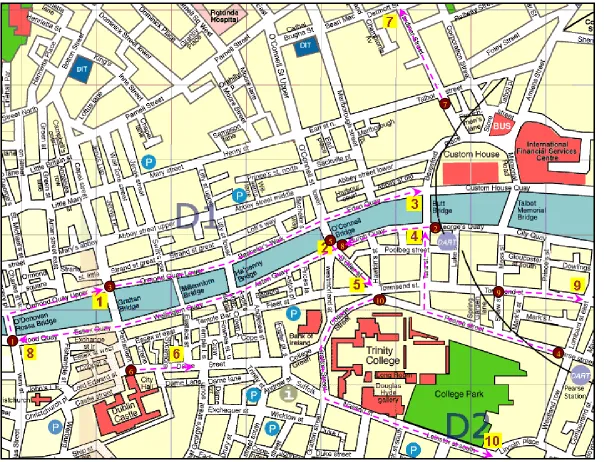
In figure 1, a map of the chosen urban transport network at the city-centre of Dublin is

given. The ten junctions where the multivariate time-series model is applied for

short-term traffic volume simulation and prediction are shown with numbered yellow

squares in the map. In the figure, the direction of the univariate traffic movement at

each intersection is shown with a pink arrow. The origin of the pink arrow is marked

with a numbered dark brown circle which signifies the nearest upstream junction to

each intersection from which traffic volume data can be obtained. The length of the

pink arrow signifies the distance between an intersection and its nearest available

upstream junctions. If this distance is considerably high then it is possible that the

changes in traffic flow at the upstream junction may not directly influence the traffic

flow at the downstream intersection.

It is evident from the figure, that the choice of the site locations at which 15 minute

traffic volume is modelled is random. The chosen intersections are not on the same

route within the transport network and none of the two stations what are the stations?

have a distance of more than 7.5 km between them?. Hence, the chosen network of

ten intersections conforms to the conditions mentioned in point one. The ten

intersections at which the proposed multivariate short-term traffic flow model is

applied for simulation and forecasting are termed as output intersections in the rest of

The traffic flow observations used for modelling from all the chosen intersections

were recorded from 3rd _{November 2003 6:30 a.m. to 26}th _{November 2003 6:30a.m.,}

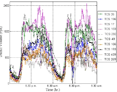
excluding the weekends. A cross-section time-series plot of the traffic flow

observations from the ten output intersections during 4th and 5th of November in 2003

is given in figure 2. The plot shows that there is a definite temporal similarity among

the curves. The output junctions at which the direction of the univariate traffic flow

fall on the routes towards the city-centre have high traffic volumes during the

morning peak hours whereas the junctions for which the same fall on the routes away

from the city-centre have higher traffic volumes during evening peak hours than the

morning peak. Consequently, the peak hourly volumes from all these ten output

junctions may not have high positive correlations, but the time of occurrence of the

maximum traffic volumes passing through the junctions are very similar. Considering

this contemporaneous correlation among the ten output traffic volume time-series

datasets, they can be modelled as panel data using SUTSE models.

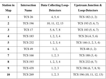
In table 1 further details about the ten output intersections are given along with the

name of the nearest upstream intersections at which traffic flow observations are

available. The 15 minute aggregate univariate traffic volumes from the mentioned

loop-detectors in the upstream junctions are used as explanatory variables in the

SUTSE model equations. In equation 5.9, the elements of the matrix _ are so chosen

that the forecasts from each intersection is affected only by the changes at its

upstream junction and not by the changes at other upstream intersections.

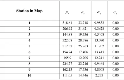
All of the ten series of traffic flow observations are modelled using homogenous

SUTSE models with equation 9 and equations 3, 4, 5 and 6 in their vector forms. The

estimated values of the trend/level component and the standard deviations of the

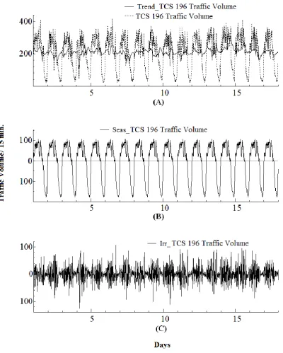
disturbances of the components are provided in table 2. The elegance of the STM lies

in the meaningful depiction of the components as shown in figure 3. In the figure,

trend, seasonality and the random error components (obtained from the traffic flow

observations collected from output station 2, as an example) are shown individually in

three different subplots. The subplot (A) shows the original traffic flow data series

along with a ? trend component as simulated and predicted from the proposed

multivariate model. The subplots (B) and (C) of the figure individually show the

seasonal and the irregular components respectively, simulated and predicted from the

MST model. The hyperparameter estimates (table 2) and the plot of the seasonal

component show that the seasonality is deterministic in nature. On the other hand the

trend component is stochastic and depicts the within-day local fluctuations in the data.

The trend component varies about a zero mean value validating the assumption that

there is no slope component latent within the traffic flow dataset.

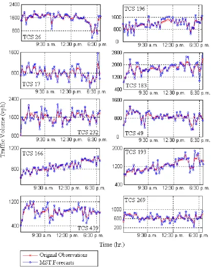
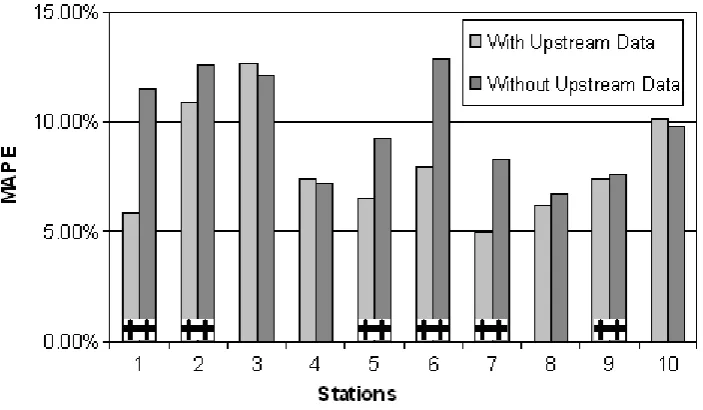
For all of the ten output junctions, 50 points in the future are forecasted (figure 4).

The traffic flow data obtained on the 26th November 2003 from 6:30 a.m. to 8:00

p.m., i.e. the data collected in the next 12.5 hours (50x15 = 750minute = 12.5hours)

are compared with these forecasts. The forecasting precision (MAPE) from the

proposed SUTSE model for each of the ten output junctions with and without

considering the influence of upstream junctions are given in figure 5 in the form of a

bar diagram. Among the ten output intersections the upstream junction is situated

indicated in the bar diagram by a coupling sign shown on the bars. It is observed

from figures 4 and 5 that the MAPE values for the forecasts at these output stations

improve significantly when the traffic flow observations from the nearest available

upstream junctions are incorporated in the SUTSE model as explanatory variables.

The forecasting precision for the remaining four output junctions do not improve

when the traffic flow observations from the nearest available upstream junction are

incorporated in the model. These are the junctions not having any upstream junction

nearby from where the loop-detector observations can be available. In such cases, the

traffic flow at the nearest upstream junction do not directly influence the traffic at the

output station due to the presence of excessive merging and diverging manoeuvres in

between the upstream and the output junction. Hence, the inclusion of the traffic flow

at far away upstream junctions as exogenous variables in the proposed model

negatively affects the performance of the model. Thus it is preferable to ignore the

influence of the traffic volume changes at an upstream junction if it is not located at

an immediate vicinity of the output station. I think it would be important to try to

justify why this is.

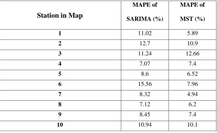
The MAPE values from the univariate SARIMA (2,0,1)(0,1,1)96 (Ghosh et al. 2005)

model for the traffic flow observations at the ten output intersections is shown in table

3 in comparison to the MAPE values from the proposed MST model for the same

junction. In most of the cases, the proposed multivariate traffic flow time-series model

prove to be more accurate than the ordinary univariate SARIMA model for short-term

simulation and forecasting of traffic volume in a congested urban network.

In this paper a structural time-series methodology is applied to develop a multivariate

short-term traffic flow forecasting model for an urban signalized transport network.

This is the first instance of applying STM to short-term traffic condition related

studies. I think you would need to include how the results from STM might compare

with other models here as the reader will be looking for comparisons. This will help

justify the use of this technique and its advantages. The model developed in the paper

is observed to have achieved some distinct advantages over the existing well-known

univariate SARIMA time-series model. These are:

 The model is capable of simultaneous simulation and modelling of traffic

conditions at multiple intersections in an urban signalized transport network

where it is difficult to model the existing paths and turning movements.

 The multivariate short-term traffic condition forecasting model developed here

is computationally much simpler and performs more accurately than the most

of the existing multivariate models.

 In structural time-series model the evolution of each individual component

(trend, seasonality etc.) of the traffic flow data over time can be traced

separately. Consequently, the deterministic nature of the seasonal component

of the traffic volume observations from junctions at urban signalized arterials

 The MST model can include the effect of changes in traffic conditions at one

or more immediate upstream junctions to improve the predictions at the

downstream output junction.

The distance of the nearest available upstream junction from the output

intersection influences the forecasting precision to a certain extent. Consequently,

for developing comparatively more efficient and robust multivariate short-term

traffic flow forecasting algorithms further studies can be performed to incorporate

the movement of traffic between the upstream junctions and the forecasting sites.

REFERENCES

Ahmed, M. S. and Cook, A. R. (1979) Analysis of freeway traffic time-series data by using Box–Jenkins techniques. Transportation Research Record: Journal of the

Transportation Research Board, No.722, pp.1–9.

Chung, E. and Rosalion, N. (2001) Short Term Traffic Flow Prediction. Proceedings

of the 24th Australian Transportation Research Forum, Hobart, Tasmania.

Davis, G. and Nihan, N. (1991) Nonparametric Regression and Short-Term Freeway Traffic Forecasting. Journal of Transportation Engineering, ASCE, Vol. 117, pp. 178-188.

Durbin, J. and Koopman S. J. (2001) Time Series Analysis by State Space Methods. Oxford Statistical Science Series, Oxford University Press.

Ghosh, B., Basu, B. and O’Mahony, M. M. (2005) Time-Series Modelling for Forecasting Vehicular Traffic Flow in Dublin. 84th Annual Meeting of Transportation

Hamed, M. M., Al-Masaeid, H. R. and Bani Said, Z.M. (1995) Short-Term Prediction of Traffic Volume in Urban Arterials. Journal of Transportation Engineering, ASCE, Vol. 121(3), pp. 249–254.

Harvey, A. C. (1989) Forecasting, Structural Time Series Models and the Kalman

Filter. Cambridge: Cambridge University Press.

Kalman, R. E. (1960) A New Approach to Linear Prediction And Filtering Problems.

Transactions of the ASME - Journal of Basic Engineering, Vol. 82, pp. 35-45.

Kamarianakis, Y. and Prastacos, P. (2002) Space-Time Modelling Of Traffic Flow.

European Regional Science Association Conference. Available from

www.ersa2002.org.

Kamarianakis, Y. and Prastakos, P. (2003) Forecasting traffic flow conditions in an urban network: comparison of multivariate and univariate approaches. 82nd Annual

Meeting of Transportation Research Board, (CD-ROM), TRB, Washington, D. C.

Kirby, H. R., Watson, S. M. and Dougherty, M. S. (1997) Should We Use Neural Network Or Statistical Models For Short-Term Motorway Traffic Forecasting?

International Journal of Forecasting, Vol.13, pp. 43-50.

Koopman, S. J., Harvey, A.C., Doornik, J.A. and Shephard, N. (1999a) Structural

Time Series Analysis, Modelling and Prediction Using STAMP. London: Timberlake

consultants Press.

Koopman, S. J., Shephard, N. and Doornik, J.A. (1999b) Statistical Algorithms for

Models in State Spaceusing SsfPack 2.2 (with discussion). Econometrics Journal,

Vol. 2, pp.113-166.

Lenten, L.J.A. and Moosa, I.A. (2003) An Empirical Investigation into Long-term Climate Change in Australia. Environmental Modelling and Software, Vol. 18, pp.59-70.

Levin, M., Tsao and Y. D., (1980) On Forecasting Freeway Occupancies and Volumes. Transportation Research Record: Journal of the Transportation Research Board, No. 773, pp. 47–49.

Lingras, P., Mountford, P. (2001) Time Delay Neural Networks Designed Using Genetic Algorithms For Short-Term Inter-City Traffic Forecasting. IEA/AIE 2001, LNAI 2070, pp. 290–299.

McQueen, B. and McQueen, J. (1999) Intelligent Transportation Systems

Architecture. Artech House Publishers, Inc., U.S.A.

Smith, B. L., Demetsky, M. J. (1994) Short-Term Traffic Flow Prediction: Neural Network Approach. Transportation Research Record: Journal of the Transportation

Research Board, No. 1453, pp. 98–104.

Smith, B. L. and Demetsky, M. J. (1997) Traffic Flow Forecasting: Comparison of Modelling Approaches. Journal of Transportation Engineering, Vol. 123(4), pp. 261– 266.

Smith, B. L., Williams, B. M., and Oswald, R. K. (2002) Comparison of Parametric And Nonparametric Models for Traffic Flow Forecasting. Transportation Research,

Part C: Emerging Technologies, Vol. 10 (4), pp. 257–321.

Stathopoulos, A., Karlaftis, M. G. (2003) A Multivariate State-Space Approach for Urban Traffic Flow Modeling and Prediction. Transportation Research Part C:

Van Arem, B., Kirby, H. R., Van Der Vlist, M. J. M. and Whittaker, J. C. (1997) Recent Advances and Applications in the Field of Short-Term Traffic Forecasting.

International Journal of Forecasting, Vol.13, pp.1-12.

Vlahogianni, E. I., Golias, J. C. and Karlaftis, M. G. (2004) Short-Term Forecasting: Overview of Objectives and Methods. Transport Reviews, Vol. 24 (5), pp. 533-557.

Vlahogianni, E. I., Karlaftis, M. G. and Golias, J. C. (2005) Optimized and Meta-Optimized Neural Networks for Short-Term Traffic Flow Prediction: A Genetic Approach, Transportation Research Part C: Emerging Technologies, Vol. 13(2), pp. 211–234.

Vythoulkas, P. C. (1993) Alternative Approaches to Short-Term Traffic Forecasting for Use in Driver Information Systems. Transportation and Traffic Theory, Proceedings of the 12th International Symposium on Traffic Flow Theory and

Transportation.

West, M. and Harrison, P. J. (1997) Bayesian forecasting and dynamic models. Srpinger, New York.

Williams, B. M., Durvasula, P. K. and Brown, D. E. (1998) Urban Traffic Flow Prediction: Application of Seasonal Autoregressive Integrated Moving Average and Exponential Smoothing Models. Transportation Research Record: Journal of the

Transportation Research Board, No. 1644, pp.132–144.

Williams, B. M. and Hoel, L. A. (2003) Modelling and Forecasting Vehicular Traffic Flow as a Seasonal ARIMA Process: Theoretical Basis and Empirical Results.

Journal of Transportation Engineering, ASCE, Vol. 129(6), pp. 664-672.

Yin, H. B, Wong, S. C., Xu, J. M. and Wong, C. K. (2002) Urban Traffic Flow Prediction Using a Fuzzy-Neural Approach. Transportation Research Part C:

LIST OF FIGURES

1. Map of the Chosen Transport Network

2. Plot of Two day Traffic volumes from Ten Output Intersections

3. Plot of Individual Components of STM Model

4. Forecasts from Ten Output Intersections from the SUTSE model

Figure 1 Map of the chosen Transport Network.

1

6

5

3

4 8

9 10

7

LIST OF TABLES

1. Details of the Ten Output Sites

2. Estimates of Parameters and Hyperparameters

4.

Station in Map

Intersection Name

Data Collecting Loop-Detectors

Upstream Junction & Loop-Detectors

1 TCS 26 4, 5, 6 TCS 182 (1, 2)

2 TCS 196 10, 11, 12, 13 TCS 193 (5, 6, 7)

3 TCS 17 5, 6, 7, 8 TCS 183 (5, 6, 7)

4 TCS 183 1, 2, 3, 4 TCS 26 (4, 5, 6)

5 TCS 232 1, 2, 3, 4 TCS 146 (1, 2, 3, 4)

6 TCS 49 1, 2, TCS 48 (1, 2)

7 TCS 166 1, 2, 3 TCS 188 (3, 4)

8 TCS 193 1, 2, 3, 4 TCS 232 (6, 7)

9 TCS 439 1, 2, 3 TCS 196 (6, 7, 8, 9)

10 TCS 269 1, 2, 3 TCS 196 (10, 11, 12, 13)

Table 2 Estimates of Parameters and Hyperparameters.

Station in Map

t

 _  

1 318.61 33.718 9.9832 0.00

2 206.92 31.621 9.3628 0.00

3 144.88 19.336 6.5408 0.00

4 322.08 28.386 13.090 0.00

5 312.33 25.763 11.202 0.00

6 154.74 17.406 13.413 0.00

7 155.9 12.705 12.241 0.00

8 224.77 23.216 9.9464 0.00

9 162.13 17.536 4.8608 0.00

Table 3 Comparison of Univariate SARIMA and MST model.

Station in Map

MAPE of

SARIMA (%)

MAPE of

MST (%)

1 11.02 5.89

2 12.7 10.9

3 11.24 12.66

4 7.07 7.4

5 8.6 6.52

6 15.56 7.96

7 8.32 4.94

8 7.12 6.2

9 8.45 7.4