Short Term Traffic Flow Forecasting Using Bayesian Combined Neural Network Model

(1)

J. of Computation in Biosciences and Engineering Volume 3 / Issue 3 ISSN: 2348 – 7313

JOURNAL OF COMPUTATION IN

BIOSCIENCES AND ENGINEERING

Journal homepage: http://scienceq.org/Journals/JCLS.php

Research Article

Open Access

Short Term Traffic Flow Forecasting Using Bayesian Combined Neural Network Model

N.T. Makanjuola1_{, O.O. Shoewu}1_{, Alao, W.A}2_{, Akinyemi, L.A}1_{, Akinyan A. R}1

1 _{Department of Electronic and Computer Engineering, Lagos State University, Nigeria} 2_{Department of Industrial Maintenance, Yaba college of Technology, Nigeria} *Corresponding author: O.O. Shoewu, E-mail: [email protected]

Received: February 20, 2017, Accepted: March 26, 2017, Published: March 26, 2017.

ABSTRACT:

In this Work, an artificial neural network model is introduced that combines the prediction from single neural network predictors according to an adaptive and heuristic credit assignment algorithm based on the theory of conditional probability and Bayes’ rule. Two single predictors are applied and combined linearly into a Bayesian combined neural network model. The credit value for each predictor in the combined model is calculated according to the proposed credit assignment algorithm and largely depends on the accumulative prediction performance of these predictors during the previous prediction intervals. Three indices, i.e., the mean absolute percentage error (MAPE), the variance of absolute percentage error (VAPE), and the probability of percentage error (PPE), are employed to compare the forecasting performance. It is found that most of the time, the combined model outperforms the singular predictors.

Keywords: Back propagation neural network, Radial Basis Function Neural network, Bayesian Combined neural network model, credit value, MAPE, VAPE, PPE.

INTRODUCTION

Short-term traffic flow prediction has long been regarded as a critical concern for intelligent transportation systems. In particular, such traffic flow forecasting supports: (1) the development of proactive traffic control strategies in advanced traffic management systems (ATMS); (2) real-time route guidance in advanced traveler information systems (ATIS); and (3) evaluation of these dynamic traffic control and guidance strategies as well. In an early report on the architecture of intelligent transportation systems, it was clearly indicated that the ability to make continuous predictions of traffic flows and link travel times for several minutes into the future, using real-time traffic data, is a major requirement for providing dynamic traffic control and guidance.

Depending on the time of the forecasts, traffic flow forecasting consists of long-term and short-term [1] forecasts. Specifically, short-term traffic flow forecasts are more greatly impacted by random interference factors, experience higher uncertainty, and show less obvious patterns or regularity. This is the main reason short-term traffic flow forecasts are more difficult than middle- or long-term forecasts.

The short-term forecasting of traffic conditions has an active but somewhat unsatisfying research history [2]. Up to now a variety of methodologies have been applied to short-term traffic flow forecasting, including the multivariate time-series model [3], the Kalman filteringMethod [4], the non-parametric regression model [5] and the neural network model [6, 7]. Generally, these techniques canbe classified into statistical models (including regression models and time-series models) and artificial intelligence or neural network models.

Comparison between these models [8], however, showed that no single predictor had yet been developed that presented itself to be universally accepted as the best, and at all times, an effective traffic flow forecasting model for real-time traffic operation.

2.1 SHORT TERM TRAFFIC FORECASTING

Since the early 1980s, short-term traffic forecasting has been an integral part of most Intelligent Transportation Systems (ITS) and related research. It concerns predictions made from few seconds to possibly few hours into the future based on current and past traffic information. Short-term prediction of traffic variables such as traffic speed, volume, flow, travel time and occupancy based on real time data, is one of the main fields to reduce traffic congestion, mobility improvement, energy saving, enhancing air quality and providing dynamic traffic control strategies.The field of short-term traffic forecasting has a life of 35 years ; in the first part of its development, most – if not all – of the research employed ‘classical’ statistical approaches to predicting traffic at a single point. Later, applications of data driven approaches were the focal point in the literature, where a rich variety of algorithmic specifications – most times creatively applied – were proposed.

2.2 ARTIFICIAL INTELLIGENCE IN TRAFFIC

FORECASTING

Artificial Intelligence (AI) is the key technology in many of today’s transportation applications (Miles and Walker, 2006). The advantage of AI applications over other alternatives lies in their interdisciplinary nature and ability to straight forwardly combine forecasts, ease of modeling and computing, and relative associated autonomy (Karlaftis and Vlahogianni, 2011). There has been increased interest among both researchers and practitioners for exploring the feasibility of applying artificial intelligence (AI) models in improving the efficiency, safety, and environmental-compatibility of transportation systems (Sadek, 2007). Such applications have not been developed as standalone systems that can cover the full range of processes involved in prediction schemes, including data collection and storage, analysis, prediction, decision making; this may limit their efficiency. (Chowdhury and Sadek, 2012) discuss the skepticism among transportation practitioners regarding the ability of AI to help solve some of the problems they face.

(2)

J. of Computation in Biosciences and Engineering Volume 3 / Issue 3 ISSN: 2348 – 7313 Artificial Neural Networks represent a branch of science that

imitates biological neural networks with the help of computers. The network can acquire accumulated experience from past environmental data, transforming this into knowledge and storing it. Furthermore, stored knowledge can be used to construct intelligent algorithmic programs or processes for subsequent forecasts or identification. ANNs are one of the most important branches of artificial intelligence (Lo C.Y., Hou C.I. and Pai Y.Y., 2011; Issanchou S., and Gauchi J.P., 2008).

Artificial Neural Networks (ANNs) are relatively crude electronic models based on the neural structure of the brain. The brain learns from experience. Artificial neural networks try to mimic the functioning of brain. Some of these patterns are very complicated and allow us the ability to recognize individual faces from many different angles.The most basic element of the human brain is a specific type of cell, called ‘NEURON’. These neurons provide

the abilities to remember, think, and apply previous experiences to our every action.

3.0 METHODOLOGY

As indicated previously, this work uses CMS (Lagos Island) – T-Junction (Epe) road in Lagos, Nigeria as a case study. Before the commencement of calculation, collection of data was carried out. These data were collected through examination of the roads, and also the internet. An approach that combines two models together was used to test and then compared with the two singular models combined.

3.1BAYESIAN COMBINATION APPROACH

The Bayesian combination approach is a type of method that tries to combine several predictors based on the conditional probability and Bayes’ rule. Suppose that a traffic flow time series yt is

produced by one of the specific k time-series models ytk (k=1, 2,

.., K).

yt = ytk (yt−1, yt−2, ..., y1) + e (1) where yt=actual traffic flow rate

in time interval t; ytk=Kth forecasting model; e=corresponding

forecast error. However, in each time interval, Eq. (1) will hold true for only one value of k and most of the time, the correct or “best” model cannot be identified in advance. A variable Z is therefore introduced to express this uncertainty, and Z is assumed to take one of the k values (1, 2, ..., K) in each time interval. With Bayes’ rule,

Ptk =

𝑃𝑟𝑜𝑏 (_{𝑦𝑡−1,…,𝑦1}𝑦𝑡, 𝑍=𝑘) ∑𝐾𝑚=1𝑃𝑟𝑜𝑏(_{𝑦𝑡−1,…,𝑦1}𝑦𝑡,𝑍=𝑚 )

(2)

and the fact that

Prob (yt, Z = k/yt−1,yt−2, ...,y1)

= Prob (yt/yt−1, yt−2, ...,y1, Z = k) · pt−1k (3)

and assuming that etk=yt−ytk is a Gaussian white noise time series

with zero mean and standard deviation 𝜎k, then

Prob (yt/yt−1, . . . ,y1, Z = k) = Prob (etk = yt – ytk/yt−1, . . . ,y1, Z = k) = 1 √2⊼𝜎𝑘𝑒 −[(𝑦𝑡−𝑦𝑡𝑘_𝜎𝑘 )]² (4) Combining Eqns. (2), (3), and (4) yields, Ptk= 1 √2⊼𝜎𝑘𝑝𝑘 𝑡−1 . 𝑒 −[(𝑦𝑡−𝑦𝑡𝑘)_𝜎𝑘 )]² ∑ 1 √2⊼𝜎𝑚𝑝𝑚 𝑡−1 . 𝑒 −[(𝑦𝑡−𝑦𝑡𝑚)_𝜎𝑚 )]² 𝐾 𝑚=1 (5)

Eq. (5) expresses the probability that model k generates the observed traffic flow rate series, which is also the credit value assigned to the Kth predictor in the combined model. Such a credit

assignment algorithm is an adaptive and heuristic scheme, which depends on observations up to time t and the prediction performance of all predictors in previous intervals. The prediction

result in time interval t+1 generated by the combined model is written as the linear combination of output of the K predictors as the following formula: Based on the Bayesian combination approach theory, the developed two single neural network predictors are combined linearly into the BCNN model with a credit for each predictor.

According to equation 5, the credit value is calculated as the posterior probability for the traffic flow time series based on the performance of the two predictors as follows:

CREDIT ASSIGNMENT ALGORITHM

Ptk= 1 √2⊼𝜎𝑝𝑡−1 𝑘 . 𝑒 −[𝑦𝑡−𝑦𝑡 𝑘_𝜎𝑘 ] 2 1 √2⊼𝜎𝑝𝑡−1 1 . 𝑒 −[𝑦𝑡−𝑦𝑡 1_𝜎1 ]2+ 1 √2⊼𝜎𝑝𝑡−1 2 . 𝑒 −[𝑦𝑡−𝑦𝑡 2_𝜎2 ]2 (6) k= 1,2 Based on equation 6, the credit values for BP and RBF neural network predictors after a time interval t (t = 1, 2…), i.e., p1

t and

p2

t, will be calculated iteratively, while p01 and p02 are chosen to be

1 for simplification.

The output of the BCNN predictor in time interval t+1 (y*t+1)is

thus formulated as: y*

t+1 = (P1t. y1t+1 + P2t . y2t+1) / 2 (7)

Where yt+11 and yt+12= respective prediction outputs of BP and

RBF neural network predictors in time interval t+1. Computational Analysis:

For,

BP (K = 1) and RBF (k = 2), 𝜎1= Standard Deviation (BP), 𝜎2= Standard Deviation (RBF) 𝜎1 = 9.43, 𝜎2 = 9.49 At t =0 and k = 1, p01 = 1 t = 0 and k = 2, p02 = 1 At t = 1, k =1 p11 = 0.13 ∗ 1 0.13 ∗ 1 + 0.13 ∗ 1 , p1 1_{= 0.5} k = 2 p12 = 0.13 ∗ 1 0.13 ∗ 1 + 0.13 ∗ 1, p1 2_{= 0.5} At t = 2, k = 1 p1 2 = 0.13 ∗ 0.5 0.13 ∗ 0.5 + 0.13 ∗ 0.5 , p2 1_{= 1} k = 2 p2 2 = 0.13 ∗ 0.5 0.13 ∗ 0.5 + 0.13 ∗ 0.5 , p2 2 _{= 1} At t = 3, k = 1 p1 3 = 0.13 ∗ 1 0.13 ∗ 1 + 0.13 ∗ 1 , p3 1_{= 0.5} t = 3, k = 2 p2 3 = 0.13 ∗ 1 0.13 ∗ 1 + 0.13 ∗ 1 , p3 2_{= 0.5} At t = 4, k = 1 p41 = 0.13 ∗ 0.5 0.13 ∗ 0.5 + 0.13 ∗ 0.5 , p4 1_{= 1} k = 2 p42 = 0.13 ∗ 0.5 0.13 ∗ 0.5 + 0.13 ∗ 0.5 , p4 2_{= 1}

The outputs of the BCNN: yt+1* = [(pt1 . yt+11)+ (pt2 . yt+12)] / 2 At t = 0, y* 1= [(p01 . y11)+ (p02 . y12)]/ 2 y* 1= (1*1250 + 1*1300) / 2 y* 1= 1275 At t = 1, y* 2= p11 . y21 + p12 . y22 y*2= 0.5 . 1150 + 0.5 . 1250 y* 2 = 1200 At t = 2, y*3 = p21 . y31 + p22 . y32 /2

(3)

J. of Computation in Biosciences and Engineering Volume 3 / Issue 3 ISSN: 2348 – 7313 y*3= (1 . 1100 + 1. 1250)/ 2 y*3= 1175 At t = 3, y* 4 = p31 . y41 + p32. y42 y* 4= 0.5 . 1100 + 0.5 .1200 y* 4= 1150 At t= 4, y* 5 = p41 . y51 + p42 . y51 y* 5= (1. 1150 + 1. 1200 y* 5 = 1175

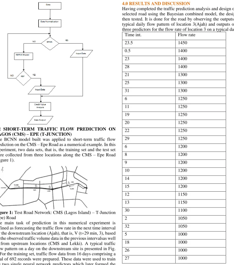
CREDIT ASSIGNMENT ALGORITHM FLOWCHART

3.2 SHORT-TERM TRAFFIC FLOW PREDICTION ON LAGOS (CMS) – EPE (T-JUNCTION)

The BCNN model built was applied to short-term traffic flow prediction on the CMS – Epe Road as a numerical example. In this experiment, two data sets, that is, the training set and the test set were collected from three locations along the CMS – Epe Road (Figure 1).

Figure 1: Test Road Network: CMS (Lagos Island) – T-Junction (Epe) Road

The main task of prediction in this numerical experiment is defined as forecasting the traffic flow rate in the next time interval for the downstream location (Ajah), that is, V (t+29 min, 3), based on the observed traffic volume data in the previous intervalsas well as from upstream locations (CMS and Lekki). A typical traffic flow pattern on a day on the downstream site is presented in Fig. 1. For the training set, traffic flow data from 16 days comprising a total of 692 records were prepared. These data were used to train the two single neural network predictors which later formed the

BCNN prediction. Next, the data from four other observation days, comprising 152 records, were used to test BCNN performance and compare the performances of the following three models, i.e., the BP neural network, the RBF neural network, and the BCNN, after they were applied to the prediction for the test data set.

The BCNN prediction for the traffic flow rate in the next time interval was based on the output value of the two neural network predictors in that interval, as well as the observed output value up to the current interval. In each time interval, the observed output was compared to the predicted outputs of the neural network predictors to determine the conditional posterior probability. 4.0 RESULTS AND DISCUSSION

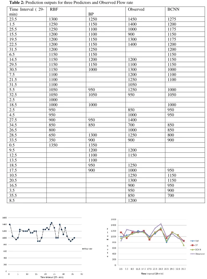
Having completed the traffic prediction analysis and design of the selected road using the Bayesian combined model, the design is then tested. It is done for the road by observing the outputs of a typical daily flow pattern of location 3(Ajah) and outputs of the three predictors for the flow rate of location 3 on a typical day.

Time int. Flow rate

23.5 1450 0.5 1400 23 1400 28 1400 21 1300 25 1300 31 1300 6 1250 11 1250 19 1250 20 1250 22 1250 29 1250 6 1200 8 1200 9 1200 10 1200 14 1200 15 1200 12 1150 13 1150 30 1100 2 1050 32 1050 5 1000 18 1000 26 1000 27 1000

(4)

Table 2: Prediction outputs for three Predictors and Observed Flow rate Time Interval ( 29-min) RBF BP Observed BCNN 23.5 1300 1250 1450 1275 1.5 1250 1150 1400 1200 25.5 1250 1100 1000 1175 15.5 1200 1100 900 1150 19.5 1200 1150 1300 1175 22.5 1200 1150 1400 1200 31.5 1200 1250 1200 6.5 1150 1150 1150 14.5 1150 1200 1200 1150 29.5 1150 1150 1100 1150 30.5 1150 1000 1300 1000 7.5 1100 1200 1100 21.5 1100 1250 1100 31.5 1100 1050 5.5 1050 950 1250 1000 32.5 1050 1050 950 1050 2.5 1000 18.5 1000 1000 1000 2.5 950 850 950 4.5 950 1000 950 27.5 900 950 1400 34.5 850 850 700 850 26.5 800 1000 850 28.5 650 1300 1250 800 33.5 350 900 900 900 0.5 1350 1350 9.5 1200 1200 12.5 1100 1150 13.5 1100 18.5 950 1250 17.5 900 1000 950 10.5 1250 1150 20.5 1300 1150 16.5 900 950 3.5 950 900 35.5 850 700 8.5 1200

Figure 1: Typical daily traffic flow pattern of Location 3 (Ajah) Figure 2: Prediction outputs of three predictors for traffic flow of Location 3 on one day

(5)

J. of Computation in Biosciences and Engineering Volume 3 / Issue 3 ISSN: 2348 – 7313 Figure 2 presents the prediction outputs of three predictors for the

traffic flow rate of Location 3 on a typical day. The observed traffic flow on that day is also presented for comparison. As shown in the results, with the exception of the RBF model in the last few intervals, all three predictors showed a good reflection of the changing trends of traffic flow, while the BCNN predictor gave the best approximation of the actual traffic flow pattern.

Three indices, that is, the mean absolute percentage error (MAPE), the variance of absolute percentage error (VAPE), and probability of percentage error (PPE), were selected and employed to compare the forecasting performances of the three aforementioned models. As the MAPE and VAPE reflect the accuracy and stability of the predictor, the probability of percentage error, i.e., PPE, indicates the reliability of the prediction. The MAPE and VAPE are defined as follows: 𝑀𝐴𝑃𝐸 =∑ ( 𝑎𝑏𝑠[𝑉(𝑡+1)−Ṽ(𝑡+1)] 𝑉(𝑡+1) ) 𝑁−1 𝑡=0 𝑁 (8) 𝑉𝐴𝑃𝐸 =√𝑁 ∑ (𝑎𝑏𝑠[𝑉(𝑡 + 1) − Ṽ(𝑡 + 1)]_{𝑉(𝑡 + 1)} ) 2 − [∑𝑁−1(𝑎𝑏𝑠[𝑉(𝑡 + 1) − Ṽ(𝑡 + 1)_{𝑉(𝑡 + 1)} )]² 𝑡=0 𝑁−1 𝑇=0 𝑁(𝑁 − 1) (9)

where V(t+1)=observed traffic volume in time interval t+1; Ṽ(t+1)=predicted traffic volume in time interval t+1; N=number of intervals for prediction. Eq. (4.1) calculates the average relative error between the prediction output and actual observed data, which represents the accuracy of the prediction. The calculation of Eq. (8) represents the sum of the deviations from the average performance during the prediction in all intervals. It is obvious that a predictor with a large VAPE is not as stable as one with a smaller VAPE.

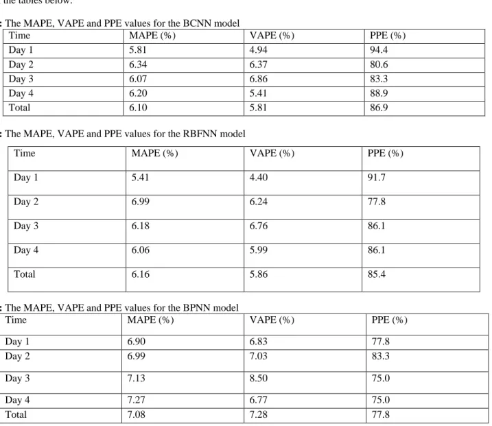
The traffic volumes collected from the four-day observation period were incorporated into the test data set and used for prediction and comparison among the three models which were built. The MAPE, VAPE, and probability of percentage error of these predictors are found in the tables below.

Table 3: The MAPE, VAPE and PPE values for the BCNN model

Time MAPE (%) VAPE (%) PPE (%)

Day 1 5.81 4.94 94.4

Day 2 6.34 6.37 80.6

Day 3 6.07 6.86 83.3

Day 4 6.20 5.41 88.9

Total 6.10 5.81 86.9

Table 4: The MAPE, VAPE and PPE values for the RBFNN model

Table 5: The MAPE, VAPE and PPE values for the BPNN model

Day 1 6.90 6.83 77.8

Day 2 6.99 7.03 83.3

Day 3 7.13 8.50 75.0

Day 4 7.27 6.77 75.0

Total 7.08 7.28 77.8

Day 1 5.41 4.40 91.7

Day 2 6.99 6.24 77.8

Day 3 6.18 6.76 86.1

Day 4 6.06 5.99 86.1

(6)

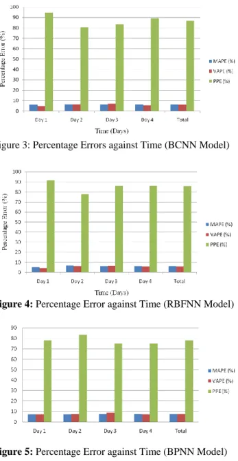
J. of Computation in Biosciences and Engineering Volume 3 / Issue 3 ISSN: 2348 – 7313 Figure 3: Percentage Errors against Time (BCNN Model)

Figure 4: Percentage Error against Time (RBFNN Model)

Figure 5: Percentage Error against Time (BPNN Model) DISCUSSION OF RESULTS AND INTERPRETATION From Tables 3, 4 and 5, it can be seen that in a four-day prediction, the BCNN predictor has a better prediction performance than the other two single neural network predictors on most days in terms of accuracy and stability, which is indicated by their MAPE and VAPE values. The performance of the BCNN predictor is not as good as those of the two predictors on some days due to a slight difference as a result of one of the two predictors yielding a better performance than the other, causing the combined model to be inclined to keep following the behavior of that model only. If each of the two predictors has a better performance during partial periods of a particular day, then the combined model would integrate their good performances together into a model with higher accuracy and better performance. It is also found that on nearly all four days, the BCNN gave a more reliable prediction, as it showed a probability of days more than 85% (up to 90%) of yielding prediction outputs with a forecasting error margin of less than 10%. This was higher than those of the other two predictors. With such a level of accuracy, the combined model could be considered as suitable input for short-term traffic scenario construction for the whole network, to be used as the foundation and traffic environment for development of proactive traffic

control strategies in ATMSs and real-time route guidance in ATISs. In all, the BCNN predictor performs better than the BP and RBF neural network predictors and is a potential model for field implementation.

5.0 CONCLUSION

In this study, two neural network predictors and a combined neural network model known as the BCNN, which is based on the Bayesian combination approach, were developed for short-term freeway traffic flow prediction. It was found that for more than 85% of time intervals, the proposed BCNN model outperformed the single predictors. Its mean absolute percentage error and variance of absolute percentage error were comparatively low. As it cannot be known in advance which particular predictor will yield the best prediction in a specific time interval. It is precisely the role of the BCNN model in tracking predictor performance online, and selecting and combining the best-performing predictors for prediction.

5.1 RECOMMENDATION

Traffic time prediction will be very useful for the residents of Lagos State to plan effectively, and to avoid unnecessary time wastage on the road. It is therefore concluded that this work can be adapted to other roads in Lagos State to help in reducing the problem of congestion in Lagos State. With only few modifications, this work can be applied on any route in the world. REFERENCES

1. 1.Smith B.L. and, Demestky M.J., “Traffic Flow Forecasting: Comparison of Modeling Approaches”, Journal ofTransportation Engineering, (1997), 261-266.

2. VIahogianni, E.I.; Golias, J.C. & Karlaftis,M.G. Short-term traffic forecasting: Overview of objectives and methods, 2004. 3. Chandra, S.R., Al-Deek, H., 2008. Cross-correlation analysis and multivariate prediction of spatial time series of freeway traffic speeds. Transportation Research Record 2061, 64–76. 4. Y. Xie, Y. Zhang, and Z. Ye, “Short-term traffic volume

forecasting using Kalman filter ”Comput.-Aided Civil Infrastruct. Eng., vol. 22, no. 5, pp. 326–334, Jul. 2007. 5. Haworth, J., Cheng, T., 2012. Non-parametric regression for

space–time forecasting under missing data. Computers, Environment and Urban Systems 36 (6), 538–550.

6. Tsai, T.-H., Lee, C.-K., Wei, C.-H., "Neural network based temporal feature models for short-term railway passenger demand forecasting". Expert Systems with Applications 36, 2009, pp.3728–3736.

7. Dharia, A. &Adeli, H. 2003, "Neural network model for rapid forecasting of freeway link travel time", Engineering Application of Artificial Intelligence, vol. 16, no. 7, pp. 607-613.

8. Karlaftis M.G., Vlahogianni E.I. "Statistical methods versus neural networks in transportation research: Differences, similarities and some insights". Transportation Research Part C 19, 2011, pp. 387-39.

9. Miles, J.C., Walker, A.J., 2006. The potential application of artificial intelligence in transport.IEEE Proceedings – Intelligent Transport Systems 153 (3), 183.

10. Chowdhury, M., Sadek, A.W., 2012. Advantages and limitations of artificial intelligence. Artificial Intelligence Applications to Critical Transportation Issues 6.

11. Sadek, A.W., (Ed.), 2007. Artificial Intelligence in Transportation: Information for Application. Transportation Research Board Circular (E-C113), TRB, National Research Council, Washington, D.C.

(7)

7

Citation: O.O. Shoewu, et al. (2017). Short Term Traffic Flow Forecasting Using Bayesian Combined Neural Network Model. J. of

Computation in Biosciences and Engineering. V3I3. DOI: 10.15297/JCLS.V3I3.01

License, which permits unrestricted use, distribution, and reproduction in any medium, provided the original author and source are credited