http://wrap.warwick.ac.uk/
Original citation:
Langwallner, B., Ortner, C. and Süli, E. (2013) Atomistic-to-continuum coupling
approximation of a one-dimensional toy model for density functional theory. Multiscale
Modeling & Simulation, Volume 11 (Number 1). pp. 59-91.
Permanent WRAP url:
http://wrap.warwick.ac.uk/54376
Copyright and reuse:
The Warwick Research Archive Portal (WRAP) makes this work of researchers of the
University of Warwick available open access under the following conditions. Copyright ©
and all moral rights to the version of the paper presented here belong to the individual
author(s) and/or other copyright owners. To the extent reasonable and practicable the
material made available in WRAP has been checked for eligibility before being made
available.
Copies of full items can be used for personal research or study, educational, or
not-for-profit purposes without prior permission or charge. Provided that the authors, title and
full bibliographic details are credited, a hyperlink and/or URL is given for the original
metadata page and the content is not changed in any way.
Publisher’s statement:
© SIAM
http://dx.doi.org/10.1137/110857787
A note on versions:
The version presented in WRAP is the published version or, version of record, and may
be cited as it appears here.
ATOMISTIC-TO-CONTINUUM COUPLING APPROXIMATION OF A ONE-DIMENSIONAL TOY MODEL FOR DENSITY FUNCTIONAL
THEORY∗
B. LANGWALLNER†, C. ORTNER‡, AND E. S ¨ULI†
Abstract. We consider an atomistic model defined through an interaction field satisfying a variational principle and which can therefore be considered a toy model of (orbital-free) density functional theory. We investigate atomistic-to-continuum coupling mechanisms for this atomistic model, paying special attention to the dependence of the atomistic subproblem on the atomistic region boundary and the boundary conditions. We rigorously prove first-order error estimates for two related coupling mechanisms.
Key words. atomistic models, quasicontinuum method, coarse graining
AMS subject classifications.65N12, 65N15, 70C20
DOI.10.1137/110857787
1. Introduction. The quasicontinuum (QC) method and, more generally, atom-istic/continuum (a/c) coupling methods are numerical coarse-graining techniques for the efficient simulation of phenomena and processes in materials at the nanoscale, such as defects, fracture, grain boundaries, or nanoindentation [18, 19, 16, 11]. In-compatibilities between the treatment of forces in atomistic and continuum models lead to difficulties in defining coupling mechanisms that do not introduce additional errors. Substantial effort has been made to understand this problem and to construct efficient and accurate a/c methods; see [17, 4, 15, 9, 20] for examples of formulations of computational methods and [1, 2, 3, 12, 13, 14] and the references therein for exam-ples of analytical treatments. Formulations of a/c methods for atomistic models based on quantum mechanics were proposed in [8, 6], but, to the best of our knowledge, no rigorous analysis of these methods exists.
In the present article we formulate and analyze one-dimensional a/c methods for an atomistic model that is defined through an interaction field satisfying a linear variational principle. Our results are related to two classes of a/c methods: First, our work can be viewed as an analysis of (a simplified version of) the a/c method proposed by Iyer and Gavini [9], who use field-based versions of classical potentials to formulate their method. Second, the atomistic model we formulate can be considered a toy model of (orbital-free) density functional theory, and hence our work represents a preliminary step towards a rigorous analysis of the a/c methods described in [8, 6]. Our main results, stated in Theorems 5.5 and 6.6, are a priori error estimates for two closely related a/c couplings. While in a comparatively simple setting, the technical steps leading up these theorems address several important issues relevant for a/c coupling in the presence of fields, most prominently the dependence on the
∗Received by the editors December 5, 2011; accepted for publication (in revised form) September
17, 2012; published electronically January 10, 2013. This work was supported by the EPSRC Critical Mass Programme “New Frontiers in the Mathematics of Solids” (OxMoS) and the EPSRC Grant “Analysis of Atomistic-to-Continuum Coupling Methods.”
http://www.siam.org/journals/mms/11-1/85778.html
†Mathematical Institute, Oxford OX1 3LB, UK ([email protected], [email protected].
uk).
‡Mathematics Institute, University of Warwick, Coventry CV47AL, UK ([email protected].
uk).
choice of boundary and boundary data for the interaction fields.
The article is structured as follows. In section 1 we formally motivate the atomistic model and introduce the necessary notation. In section 2 we give a precise formulation of the model with periodic boundary conditions and derive a “weak formulation” for the resulting forces on the particles. Section 3 is devoted to the analysis of the model in a bounded domain when the fields are subjected to Dirichlet boundary conditions. The Cauchy–Born continuum model is derived and analyzed in section 4. Finally, in sections 5 and 6 we propose two possible constructions of a/c methods based on different exchanges of boundary conditions between an atomistic and a continuum region, and we establish error estimates.
We will occasionally cite the extended preprint [10] to refer to details of certain arguments that we have omitted from the present work.
1.1. Field-based formulation of pair interactions. The following outline follows ideas presented in [9]. Let y = (y1, . . . , yN)∈ RN represent the coordinates of N particles in one dimension. We consider an atomistic energy based on a pair-potentialV,
E(y) =1 2
N
i,j=1
i=j
V(|yi−yj|).
The force on particleiis given by
−DyiE(y) =−
N
j=1
j=i
sign (yi−yj)V(|yi−yj|).
We note that the forces are nonlocal expressions in the sense that their computation involves summation over the otherN−1 particles.
Next, we make a few modifications to this model. First, we replace the pointwise particles with smooth, nonnegative, and compactly supported particle densitiesδε(·−
yi) (such that
Rδε(x) dx= 1). This leads to
E(y)≈1 2
N
i,j=1
i=j
R
R
δε(z−yi)V(|z−x|)δε(x−yj) dzdx.
To simplify the presentation further, we include the self-energies of the individual particle densities and define
Eε(y) = 1 2
N
i,j=1
R
R
δε(z−yi)V(|z−x|)δε(x−yj) dzdx.
This additional self-energy contribution does not affect the forces. It can be computed explicitly and subtracted from the energy later on. Upon introducing the fieldφ:R→
R,
(1.1) φ(x) =
R
ρy(z)V(|x−z|) dz, where ρy(z) = N
i=1
we can rewrite the energyEε(y) in the form
Eε(y) = 1 2
R
ρy(x)φ(x) dx.
It is now easy to see that the forces are given by thelocal expression
−DyEε(y) =−
R
Dyρy(z)φ(z) dz.
Hence, if the field φ is known, then it becomes unnecessary to compute nonlocal sums over particles. The nonlocality of the interaction has been encoded in the field
φ. However, it is now necessary to compute the field φ, which is defined via the convolution (1.1).
Suppose that the pair-potentialV is the Green’s function for a linear differential operator LV(∇); then, φ can alternatively be computed by solving the differential equation
LV(∇)φ=ρy.
As an example we consider the Yukawa potential in one space dimension
V(x) = 1 2me
−m|x|= 1 2π
R
1
k2+m2e ikxdk.
In this caseφcan be obtained as the solution to
−Δφ+m2φ=ρy
or, equivalently, as a solution to the minimization problem
φ= arg min ϕ
1 2
R|∇
ϕ|2+m2ϕ2dx−
R ρyϕdx
.
The resulting interaction potentialEεcan also be written in the form
(1.2) Eε(y) =−min ϕ
1 2
R|∇
ϕ|2+m2ϕ2dx−
R ρyϕdx
.
The present work is devoted to the analysis of a/c approximations of (1.2) in a periodic one-dimensional setting. What distinguishes this analysis from previous analyses of a/c methods is that the coupling is achieved through an exchange of boundary conditions for the interaction fieldφ, rather than ghost-force removal ideas such as in [4, 15].
Remark 1. The interaction defined by (1.2) is purely repulsive. A purely at-tractive interaction can be obtained by changing the outer minus sign in the defini-tion of Eε to a plus sign. We could take linear combinations of the two energies of the form (1.2) with different parameters m to obtain a Morse potential interaction:
V(x) = e−2m(|x|−1)−2e−m(|x|−1)=C2e−2m|x|−2Ce−m|x|, where C = em. Indeed, following [9, sect. 4.1] we can show that, with this choice,
Eε(y) = 1 2
N
i,j=1
R
R
δε(z−yi)V(|z−x|)δε(x−yj) dzdx
= inf ϕ
R
1 2|∇
2ϕ|2+m2|∇ϕ|2+1
2α
4|ϕ|2−ρ
yϕ
In particular, the field φcan now be obtained by solving a fourth-order differential equation. We anticipate no difficulties in generalizing our analysis to this case.
Even after introducing an attractive potential, our methods seem rather limited in their scope. We remark, however, that more general pair interactions can be approximated by linear combinations of exponential potentials [9].
Many-body interactions lead into the field of orbital-free density function theory. Generalizing our analysis to that extent would require more substantial modifications.
1.2. Notation. We consider an infinite chain of atoms on the one-dimensional lattice X = εZ, where ε = 2/(2N + 1) is the reference lattice spacing. Moreover, to keep the analysis simple, we admit only (2N+ 1)-periodic displacements from the reference lattice (cf. [14]). Hence, we define the spaces of admissible displacements and deformations, respectively, by
U =u∈RZ:uj+(2N+1)=uj ∀j∈Z, N
j=−Nuj= 0
,
Y=FX+U,
where F > 0 is a prescribed macroscopic strain. A deformation y ∈ Y defines the computational domain
Ω = (y−N−1, yN)
for the field variableφ. We note that the length of the interval is independent ofy. We define the finite differences y,y ∈ U for y ∈ Y or U by their respective components
yj= yj−yj−1
ε , y
j =
yj+1−2yj+yj−1
ε2 .
Let us also define the weighted 2 scalar product and norm by
(1.3) (u,v)ε=ε N
ν=−N
uνvν ∀u,v ∈ U, u2ε := (u,u)1ε/2 ∀u∈ U.
The ∞-norm is defined in the obvious way:
u∞= max
ν=−N,...,N|uν| ∀u∈ U.
The spaceU equipped with the discrete Sobolev seminormuU1,2 =u2ε will be denoted byU1,2 and its topological dual space byU−1,2. The norm onU−1,2 is given
by
TU−1,2 = sup
u∈U1,2 T·u
uU1,2 ,
where, due to the finite-dimensional setting, we denote the duality pairing byT·u. For monotonically increasingy ∈ Y (which we will write as y >0) we denote by S(y)⊂H1(Ω) the space of continuous functions that are linear on every interval Qi= (yi−1, yi),i∈ {−N, . . . , N}. Furthermore, we define S#(y) = S(y)∩H#1(Ω) to
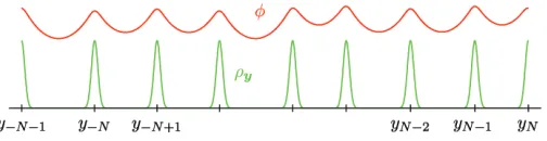
Fig. 2.1. Sketch of the basic atomistic problem: the field φis periodic inΩ = (y−N−1, yN),
andρy is a smooth particle density representing the atoms with positions given byy∈ Y.
2. Periodic boundary conditions. We now put the field-based interaction potential that was outlined above in a precise mathematical framework. Let the functionalI:H1
#(Ω)× Y →Rbe defined by
I(ϕ,y) =
Ω
1
2ε2|∇ϕ|2+12m2ϕ2
dx−
Ω
ρyϕdx, where
ρy(x) =ε
j∈Z
δε(x−yj) and δε(x) =ε−1δ1(x/ε).
Here, δ1 is a symmetric, nonnegative, regularized delta distribution with compact support −ς0
2,
ς0 2
, whereς0>0 andRδ1dx= 1; see Figure 2.1. We will frequently refer to the parameterς0, which is fixed throughout the paper.
We then define the interaction potentialE:Y →Rby
(2.1) E(y) =− min
ϕ∈H1#(Ω)
I(ϕ,y).
The respective minimizer (see Figure 2.1)
φ= arg min ϕ∈H1#(Ω)
I(ϕ,y)
is the periodic solution to the Euler–Lagrange equation
(2.2) −ε2Δφ+m2φ=ρy in Ω.
Althoughφdepends ony, we will usually suppress this in our notation. It will always be clear from the context which configurationφbelongs to. It follows from (2.2) and integration by parts that
E(y) = 1 2
Ω
φρydx.
To determine equilibrium configurations subject to a given external forcef ∈ U−1,2 (represented by the inner product (f,·)ε) we need to minimize the total potential energyEf:Y →Rdefined by
(2.3) Ef(y) =E(y) + (f,y)ε.
A minimizer ¯y∈ Y of (2.3) satisfies the following Euler–Lagrange equation inU−1,2:
In the remainder of the section we analyze the derivatives ofE. Our main result is the “weak formulation” (2.6) ofDE, mimicking the weak form of an elliptic PDE. This result acts as a natural connection to the weak form of the Cauchy–Born equation, which we will derive in section 4.
We begin by computing a more classical representation of the forces.
Proposition 2.1. The potentialE:Y →Rdefined by (2.1)is twice continuously
Fr´echet differentiable. The components of the first derivative are given by
(2.4) DyjE(y) =−ε
Ω
∇δε(x−yj)φ(x) dx
for j∈ {−N, . . . , N−1} and by
(2.5) DyNE(y) =−ε
Ω
∇δε(x−y−N−1) +∇δε(x−yN)
φ(x) dx.
Proof. The proof of this result is standard and can be found in [9], for exam-ple. The occurrence of bothyN and y−N−1in (2.5) is due to the periodic boundary condition. Note thatyN is the “periodic image” ofy−N−1.
We stress the fact that the forces −DyE(y) are local expressions. To calculate the force on atomj it is necessary to knowφin suppδε(· −yj), but there is no need to sum over all remaining atoms. This nonlocality is encoded in the field φ.
Next we establish the weak formulation for the forces on particles. A version of this calculation was already shown in [7], which used an interpolant for the displace-ment that is constant on the support of everyδε(· −yj). To avoid this restriction, we modify and extend the argument in [7]. For simplicity we assume that the supports of the densities of different particles do not intersect:
suppδε(· −yi)∩suppδε(· −yj) =∅ ∀i, j∈Z, i=j.
Removing this restriction would create substantial additional technical difficulties throughout the analysis.
Since|suppδε(· −yi)|=ες0, this is equivalent to|yj−yi|> ες0 fori=j or, ify
is an increasing sequence,yj > ς0for allj∈Z.
Lemma 2.2. Lety∈ Y satisfyy > ς0, and letφ∈H1
#(Ω)be the associated field,
defined by (2.2). Let u= (uj)j∈Z ∈ U be a test vector and u∈S#(y) be the periodic
piecewise linear interpolant of u; that is,u(yj) =uj for j∈Z. Then,
(2.6) DE(y)·u= N
j=−N
DyjE(y)·uj=
Ω
σy(x)∇u(x) dx,
whereσy=σy,1+σy,2 and
σy,1(x) = 12ε2|∇φ|2−12m2φ2+ρyφ,
σy,2(x) =ε
N
j=−N−1
φ(x)∇δε(x−yj)(x−yj). (2.7)
the componentuj:
DyjE(y)uj = −εuj
Ω
∇δε(x−yj)φ(x) dx
= −ε
Ω
u(x)∇δε(x−yj)φ(x) dx+ε
Ω
(u(x)−uj)∇δε(x−yj)φ(x) dx
=ε
Ω
δε(x−yj)u(x)∇φ(x) dx+ε
Ω
δε(x−yj)φ(x)∇u(x) dx
+ε
Ω
(u(x)−uj)∇δε(x−yj)φ(x) dx=:T( j) 1 +T(
j) 2 +T(
j) 3 .
Here we have used integration by parts, but there are no boundary terms sinceu,φ, andρy are periodic on Ω. Using (2.5) we obtain a similar expression forDyNE(y)uN. Summing overj =−N, . . . , N we obtain
(2.8) DE(y)·u= N
j=−N
DyjE(y)·uj=T1+T2+T3,
where Ti = N j=−NT
(j)
i , i ∈ {1,2,3}. Fromρy = ε j∈Zδε(· −yj) it immediately follows that
T2=
Ω
ρy(x)φ(x)∇u(x) dx.
ForT1we can carry out the following rearrangements:
T1=
Ω
ρyu∇φdx=
Ω
−ε2Δφ+m2φu∇φdx
=
Ω
−ε2∇φΔφ+m2φ∇φudx=1 2
Ω
∇−ε2|∇φ|2+m2φ2udx
= 1 2
Ω
ε2|∇φ|2−m2φ2∇udx.
Here, we have again used integration by parts and the periodicity of all functions involved. We deduce that
T1+T2=
Ω
σy,1(x)∇u(x) dx,
withσy,1as defined in (2.7).
Before turning toT3 we first note that, sinceuis piecewise linear,
u(x) =uj+
x−yj
yj−yj−1
(uj−uj−1) =uj+ (x−yj)∇u(x) forx∈Qj= (yj−1, yj),
u(x) =uj+
x−yj
yj+1−yj
(uj+1−uj) =uj+ (x−yj)∇u(x) forx∈Qj+1= (yj, yj+1).
Hence,T3 in (2.8) can be written as
T3=ε
N
j=−N−1
Ω
φ(x)∇δε(x−yj)(u(x)−uj) dx
=ε
N
j=−N−1
Ω
φ(x)∇δε(x−yj)(x−yj)∇u(x) dx= ε
Ω
withσy,2as defined in (2.7), which concludes the proof.
Remark 2. 1. In more than one space dimension the above calculations can be generalized if a triangular, respectively, tetrahedral, mesh with the atomic positions as nodes is constructed. For example, this leads to
σy,1(x) =
−1
2ε2|∇φ|2−21m2φ2+ρyφ
id +ε2∇φ⊗ ∇φ.
2. A closer look at the calculations in the proof of Lemma 2.2 shows that the weak form can be obtained for semilinear models −ε2Δφ+F(φ) = ρ
y with any convex
functionF. Even a fourth-order model of the formε4Δ2φ−ε2Δφ+F(φ) =ρ
yadmits
a similar weak formulation.
As already suggested in the introduction the Green’s function for the differential operator−ε2Δ +m2id acting on functions defined onRis given by
(2.9) Gε(x) =
1 2εme
−mε|x|.
We therefore get the following explicit formulas for the function valuesφ(x) and∇φ(x) forx∈Ω.
Proposition 2.3. Let y∈ Y, and letφ= arg minϕ
∈H#1(Ω)I(ϕ,y) be the
corre-sponding interaction field. Then, for every x∈Ω,
φ(x) =
R
Gε(x−z)ρy(z) dz= 1 2m
k∈Z
R
δε(z−yk) e− m
ε|x−z|dz, (2.10)
∇φ(x) =
R
Gε(x−z)∇ρy(z) dz= 1 2m
k∈Z
R∇
δε(z−yk) e− m
ε|x−z|dz.
(2.11)
Proof. The proof of this proposition is similar to that of [5, Thm. 2.1]; see also the extended preprint [10, Prop. 2.4].
The following is a consequence of the simple exponential form of the Yukawa potential and some elementary properties of the exponential function in one dimen-sion. Let yi, yj ∈ R satisfyyj > yi+ες0, so that the supports of particle densities
representing the atomsiand jdo not intersect. Then,
R
R
δε(z−yj) e− m
ε|z−x|δε(x−yi) dxdz
=
R
R
δε(z−yj) e− m
ε(z−x)δε(x−yi) dxdz
= e−mε(yj−yi)
R
e−mε(z−yj)δε(z−yj) dz·
R
e−mε(yi−x)δε(yi−x) dx
=μ2e−mε(yj−yi),
(2.12)
where we have defined
μ=
R
δε(x)e− m
εxdx=
R δε(x)e
m εxdx=
R
δ1(x)emxdx.
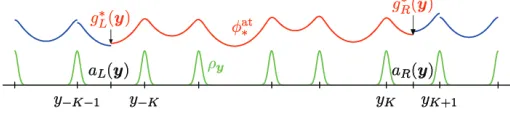
Fig. 3.1.The atomistic model in the domainΩawith Dirichlet boundary conditionsg= [gLgR]T.
3. Dirichlet boundary conditions. In this section we consider a version of the model (2.1) in the domain Ωa = (aL, aR)⊂Rsubject to Dirichlet instead of periodic boundary conditions; cf. Figure 3.1. This concept will be used in sections 5 and 6, for the formulation of a/c methods, as the atomistic subproblem. We will study the dependence of this subproblem on the choice of boundary points aL, aR and on the choice of boundary data that we prescribe for the field variableφat those points. The results we develop in this section will guide us in our treatment of the a/c interface in sections 5 and 6.
We set a= [aL aR]T∈ R2 and Δa =aR−aL. Throughout section 3 we think of y= (y−K, . . . , yK) as an ordered element of Ωa2K+1 such that aL < y−K <· · · <
yK < aR, whereK < N. The particle densityρy is defined by
ρy=ε
K
j=−K
δε(· −yj).
We shall assume throughout that the yj are separated and lie well inside Ωa in the sense that suppρy∩∂Ωa =∅ or, equivalently,
yi≥ς0 fori=−K+ 1, . . . , K,
aR−yK > ες0/2 and y−K−aL> ες0/2.
(3.1)
We impose the following boundary conditions on the resulting fieldφ: Ωa →R:
φ(aL) =gL, φ(aR) =gR;
i.e.,φ|∂Ωa =g, withg= [gL gR]T∈R2. The interaction potentialEa,g : Ω2aK+1→R is defined by
(3.2) Ea,g(y) =− min
ϕ∈H1(Ωa)
ϕ|∂Ωa=g
Ia(ϕ,y),
whereIa:H1(Ωa)×Ω2aK+1→Ris given by
(3.3) Ia(ϕ,y) = aR
aL
1
2ε2|∇ϕ|2+12m2ϕ2
dx−
aR
aL
ρyϕdx.
For givenythe minimizer φis the weak solution to
−ε2Δφ+m2φ=ρy in Ωa,
φ|∂Ωa =g. (3.4)
We will frequently use the decomposition
where φ0 ∈H1
0(Ωa) and ξa,g ∈H1(Ωa), respectively, solve the boundary-value prob-lems
−ε2Δφ0+m2φ0 =ρy in Ωa,
φ0|∂Ωa = 0
and
−ε2Δξa,g+m2ξa,g= 0 in Ωa,
ξa,g|∂Ωa =g. (3.6)
This last boundary-value problem can be solved explicitly, which yields the following lemma.
Lemma 3.1. The solutionξa,g of (3.6)is given by
(3.7) ξa,g(x) =cL(a, g)e−
m
ε(x−aL)+c
R(a, g)e−
m ε(aR−x),
where the coefficientscL(a, g)andcR(a, g)are given by
(3.8) c(a, g) =
cL(a, g)
cR(a, g)
=
1 τ τ 1
−1 gL
gR
=:Ta−1·g
and we have definedτ= exp(−mεΔa).
Note that, for Δaε,τ is exponentially small; hence we will often neglect terms of that order of magnitude. We will write O(τ) for a quantity or function that is (uniformly) bounded above byCτ in modulus, whereC is independent ofεand Δa. For example, we havec(a, g) =g+O(τ).
Next, we compute the derivative ofEa,g with respect to the atomic coordinates. For these derivatives, we obtain a “weak” formulation of the same shape as in the periodic case (see Proposition 2.1).
If y > 0, then we denote by S(y∪a) the set of continuous, piecewise affine functions over the mesh given by the nodesaL, y−K, . . . , yK, aR. Moreover,S0(y∪a) =
S(y∪a)∩H1 0(Ωa).
Proposition 3.2. Let a, g∈R2,aL< aR; thenEa,g:Y →Rdefined by (3.2)is
continuously Fr´echet differentiable at y:
(i)The components of the first derivative are given by
(3.9) DyjEa,g(y) =−ε
Ωa
∇δε(x−yj)φ(x) dx for i=−K, . . . , K.
(ii)Let u∈ U be a test vector,u∈S0(y∪a)its interpolant, and let miny ≥ς0; then,
(3.10) DyEa,g(y)·u=
Ωa
σy(x)∇u(x) dx,
whereσy is given by (2.7).
Proof. The derivatives with respect to the coordinatesy are easy to calculate along the same lines as in the proof of Proposition 2.1. The weak formulation can be obtained as in the periodic case (Lemma 2.2) using the fact that the interpolant u
Remark 3. We point out that, in general,
Ea,g(y)= 1 2
Ωa
ρyφdx.
However, we will see below, for example in (3.16), thatEa,g(y) can be written as the sum of a boundary data contribution and a term that is independent ofg.
With a view to the subsequent derivation of a/c methods we will from now on interpret a and g as arguments to Ea,g rather than fixed parameters entering its definition. We consider the map Ω2K+1
a ×R2×R2 →R, (y, a, g)→ Ea,g(y), and we obtain an expression of the derivatives of this map with respect to the boundary a
and the boundary datag.
3.1. Dependence on the boundary positions. When formulating a/c meth-ods in section 5 we will let the boundaryaof the atomistic subdomain depend on the configurationy. It is therefore necessary to understand the dependence of the energy Ea,g(y) ona. Our main result is that the derivativeDaEa,g(y) can be combined with
DyEa,g(y) into a weak formulation reminiscent of (2.6). This will be a central building block for a/c methods.
Proposition 3.3. Suppose that y ∈ Y, miny ≥ ς0. Let h = [hL hR]T ∈ R2
and u = (u−K, . . . , uK) ∈ R2K+1 be test vectors, and let u ∈ S(y∪a) denote the
interpolant ofu andhin the sense that
u(aL) =hL, u(aR) =hR, and u(yj) =uj ∀j∈ {−K, . . . , K}.
Then,
DaEa,g(y)·h+DyEa,g(y)·u=
Ωa
σy(x)∇u(x) dx,
whereσy is defined in (2.7).
Proof. This is a direct consequence of the following two lemmas and (3.10). In the first auxiliary lemma we compute the derivative of Ea,g(y) with respect to a = [aL aR]T while keeping the relative distances between the atoms constant. In other words we consider the change in Ea,g(y) when the whole domain Ωa is stretched with the atom positions following this stretching. For y ∈ Ω2K+1
a let
X = (X−K, . . . , XK) ∈ (0,1)2K+1 be given implicitly by yj = aL + ΔaXj for all
j∈ {−K, . . . , K}. For fixedg,X we define
E(a) :=Ea,g(aL+ (aR−aL)X),
DaREa,g(y) :=DaRE(a).
(We understandaL+ (aR−aL)X in a componentwise manner: (aL+ ΔaX)j =aL+ ΔaXj for allj∈ {−K, . . . , K}.) The derivativeDaLEa,g(y) is defined analogously.
Lemma 3.4. Let y∈Ω2aK+1 satisfy (3.1); then
(3.11) −DaLEa,g(y) =DaREa,g(y) = 1 Δa
Ωa
σy(x) dx.
prob-lem to the unit interval (0,1) using the transformationx→X(x) = (x−aL)/(aR−aL):
E(a) =Ea,g(η(a)) =
Ωa
−1 2ε
2|∇φ|2−1
2m
2φ2+ρ
η(a)φ
dx
= Δa
1
0
− ε2 2Δa2|∇φ|
2−m2
2 φ
2+ρ
η(a)φ
dX.
(3.12)
Here,φ(X) =φ(x(X)) andρη(a)(X) =ρη(a)(x(X)). It follows as in Proposition 2.1
that, to compute DaE(a), it is sufficient to calculate the partial derivatives of the right-hand side with respect to aR (the derivative ofφor φwith respect to aR does not appear sinceφis a minimizer ofIa(·,y)). This leads to
DaRE(a) =
1
0
− ε2 2Δa2|∇φ|
2−m2
2 φ
2+ρ
η(a)φ
dX+ Δa
1
0 ε2
Δa3|∇φ| 2dX
+ Δa
1
0
φDaRρη(a)dX.
Transforming the first two integrals on the right-hand side back to the interval Ωawe arrive at
1
ΔaEa,g(y) + ε2
Δa
Ωa
|∇φ|2dx= 1 Δa
Ωa
σy,1(x) dx,
whereσy,1 was given in (2.7).
It remains to differentiate ρη(a) with respect to aR. By the definition of the transformationx→X(x) we have
DaRρη(a)(X) =εDaR
K
j=−K
δε
(aR−aL)(X−Xj)
=ε
K
j=−K
(X−Xj)∇δε
(aR−aL)(X−Xj)
.
Using Δa(X−Xj) = (x−yj) we therefore get
Δa
1
0
φDaRρη(a)dX = ε
Δa
K
j=−K
Ωa
(x−yj)∇δε(x−yj)φ(x) dx
= 1 Δa
Ωa
σy,2(x) dx,
withσy,2(x) as given in (2.7).
To see thatDaLE=−DaREwe simply note thatE(a) depends only on Δa, which can be seen from (3.12) and the definition ofρη(a)(X).
We defineθR∈S(y∪a) to be the piecewise linear function with
θR(aR) = 1, θR(aL) = 0, θR(yj) = 0 ∀j∈ {−K, . . . , K}.
Lemma 3.5. Let y ∈Ω2aK+1 satisfy (3.1); then, the derivatives of Ea,g(y) with
respect to aL,aR (for fixed y andg) satisfy
DaLEa,g(y) =
Ωa
σy(x)∇θL(x) dx,
DaREa,g(y) =
Ωa
σy(x)∇θR(x) dx.
Proof. Let ΘRbe the affine function defined on Ωawith ΘR(aL) = 0, ΘR(aR) = 1. Since∇ΘR(x) = Δ1a, Lemma 3.4 yields
(3.13) DaREa,g(y) =
Ωa
σy∇ΘRdx=
Ωa
σy∇(ΘR−θR) dx+
Ωa
σy∇θRdx.
Now, we have ΘR−θR∈S0(y∪a) and hence, by Proposition 3.2,
(3.14)
Ωa
σy(x)∇(ΘR−θR) dx= K
j=−K
DyjEa,g(y)ΘR(yj).
However, DaREa,g(y) was defined as the derivative with respect to aR, while the relative distances of the atoms are kept constant. Thus, we see that
DaREa,g(y) =DaREa,g(y) + K
j=−K
DyjEa,g(y)ΘR(yj).
Inserting this into (3.13) and using (3.14) then gives
Ωa
σy(x)∇θRdx=DaREa,g(y).
Similarly, we can show the expression stated forDaLEa,g(y).
3.2. Dependence on the boundary values. Next, we compute the derivative of Ea,g(y) with respect to the boundary conditions g when the configuration y and the boundaryaare kept fixed. We define
γL(y, a) = 2
Ωa
ρy(x)Gε(x−aL) dx and γR(y, a) = 2
Ωa
ρy(x)Gε(aR−x) dx. (3.15)
Lemma 3.6. The partial derivative of Ea,g(y)with respect tog is given by
DgEa,g(y) =−mε
(1−τ2)
cL(a, g)
cR(a, g)
−
γL(y, a)
γR(y, a) T
·Ta−1,
whereTa,c(a, g) = [cL(a, g)cR(a, g)]T, andτ = e− m
εΔa are defined in Lemma 3.1.
Proof. Throughout the proof we suppress the arguments of γL, γR, and c for ease of readability. We recall the additive decompositionφ = φ0+ξa,g from (3.5). From φ0 ∈ H01(Ω) and from the equation −ε2Δξa,g +m2ξa,g = 0 it follows that
ε2(∇ξa,g,∇φ0) +m2(ξa,g, φ0) = 0. Hence, a short calculation shows that the energy
Ea,g(y) can be rewritten as
The first term on the right-hand side does not depend on the boundary conditionsg, and the second term is known explicitly: using −ε2Δξa,g+m2ξa,g = 0, integration
by parts, and the explicit formula (3.7) forξa,g, we obtain
Ia(ξa,g,y) =
Ωa 1 2
ε2|∇ξa,g|2+m2ξ2a,g
dx−
Ωa
ρyξa,gdx
= ε
2
2
−ξa,g(aL)∇ξa,g(aL) +ξa,g(aR)∇ξa,g(aR)
−
Ωa
ρyξa,gdx
= εm 2
c2L+c2R1−e−2mεΔa−
Ωa
ρycLe−
m
ε(x−aL)+c
Re−
m
ε(aR−x)dx
=mε
c2
L+c2R 2
1−τ2− 2
2mε
Ωa
ρycLe−
m
ε(x−aL)+c
Re−
m
ε(aR−x)dx
=mε
c2L+c2R
2
1−τ2−cLγL+cRγR
.
Here we have used the Green’s functionGεfrom (2.9). Differentiating this expression with respect to cL and cR and applying the chain rule with Dgc = Ta−1 yield the result.
A useful auxiliary result for the analysis of a/c methods is the global Lipschitz continuity of the fieldφwith respect to variations in the boundary conditionsg.
Lemma 3.7. Letφ1, φ2∈H1(Ωa)be minimizers ofIa(·,y)subject to the boundary
conditionsg1∈R2, respectively, g
2∈R2. Then,
|φ1(x)−φ2(x)| ≤ √2|Ta−1(g1−g2)|e−mεda(x),
ε|∇φ1(x)− ∇φ2(x)| ≤ √2m|Ta−1(g1−g2)|e− m
εda(x),
where da(x) := min(x−aL, aR−x) denotes the distance to the boundary of Ωa, for
x∈Ωa.
Proof. We write both functions in the formφi=φ0+ξa,gi,i∈ {1,2}. Fori= 1,2, letci=Ta−1gi be the respective coefficients enteringξa,gi; then,
|φ1(x)−φ2(x)|=|ξa,g1(x)−ξa,g2(x)| ≤ |c1,L−c2,L|e−
m
ε(x−aL)+|c1,R−c2,R|e− m
ε(aR−x).
This immediately yields the first bound. The bound for the derivatives is obtained similarly.
3.3. “Optimal” boundary conditions. In this subsection we study a specific choice of boundary datag that will play an important role throughout the remainder of the paper.
We begin by noting thatDgEa,g(y) = 0 if and only if
cL(a, g) =γL(y, a)/(1−τ2) and cR(a, g) =γR(y, a)/(1−τ2).
According to (3.8) this corresponds to the boundary conditions
(3.17) g∗L= 1 1−τ
γL+τ γR
1 +τ and g ∗
R=
1 1−τ
τ γL+γR 1 +τ .
boundary conditionsg=g∗(y, a) minimize the boundary data contributionIa(ξa,g,y) to the energy Ea,g(y). This is equivalent to minimizing Ia(·,y) over H1(Ωa) and therefore leads to homogeneous Neumann boundary conditions forφon∂Ωa.
If Δa ε, i.e., τ 1, then we have γL/R = gL/R∗ +O(τ), and hence we can simplify
Ia(ξa,g,y) =mε 1
2
gL2+g2R
−gLg∗L+gRg∗R
+O(ετ),
(3.18)
DgEa,g(y) =mε(g∗−g) +O(ετ).
In the remainder of this subsection, we take a closer look at the interaction po-tentialEa,gfrom (3.2) with they-dependent boundary conditionsg=g∗(y, a) defined in (3.17).
Proposition 3.8. Lety∈Ω2aK+1. Then,
Ea,g∗(y,a)(y) =
1 4mε
Ωa
Ωa
ρy(x)e− m
ε|x−z|ρy(z) dzdx+τ Mτ(γL, γR)
+ 1 4mε
Ωa
Ωa
ρy(x)e− m
ε(2aR−x−z)+ e− m
ε(x+z−2aL)ρy(z) dzdx,
(3.19)
whereMτ(γL, γR)depends quadratically on γL andγR.
Expression (3.19) can be interpreted as the energy of the atoms represented byy interacting with each other plus the interaction with mirror atoms outside Ωa. This mirror interaction was introduced by means of the boundary conditionsg=g∗.
For the proof of the proposition it is convenient to use an explicit formula for the function values of φ0 ∈ H1
0(Ωa) from the decomposition (3.5). By Proposition 2.3, the Green’s function for the equation −ε2Δφ+m2φ = ρ
y in R is given by
Gε(x, y) = 2mε1 e−
m
ε|x−y|. We will now construct the Green’s function Gε,a for the operator−ε2Δ +m2id subject to homogeneous Dirichlet conditions on∂Ωa.
Lemma 3.9. Let φ0∈H1
0(Ωa)satisfy −ε2Δφ0+m2φ0=ρy inΩa. Then,
(3.20) φ0(x) =
Ωa
Gε,a(x, z)ρy(z) dz ∀x∈Ωa,
whereGε,a=G(1)ε,a+τ G(2)ε,a, withG(ε,ai),i= 1,2, given by
G(1)ε,a(x, z) = 1 2mε
e− m
ε|x−z|−e− m
ε(x+z−2aL)−e− m
ε(2aR−x−z)
,
G(2)ε,a(x, z) = − 1 2mε
1 1−τ2
τe− m
ε(x+z−2aL)+τe− m
ε(2aR−x−z)
−e−mε(x−z+aR−aL)−e−mε(z−x+aR−aL)
.
Proof. The proof of this result is standard [5, Chap. 2.2.4]; see also [10, Lem. 3.10].
We remark thatGε,a=G(1)ε,a+O(τ).
Proof of Proposition 3.8. We have already seen in (3.16) that for any choice of boundary datag∈R2 the energyEa,g(y) can be written as the sum of two terms
Ea,g(y) =−Ia(φ,y) =−Ia(φ0,y)−Ia(ξa,g,y),
Calculation of Ia(φ0,y). Since the function φ0 is a minimizer of Ia(·,y) over
H1
0(Ω), we have with the expression (3.20) forφ0(x) that
(3.21) Ia(φ0,y) =−
1 2 Ωa Ωa
ρyφ0dx=−1 2
Ωa
Ωa
ρy(x)Gε,a(x, z)ρy(z) dzdx.
By the definition (3.15) ofγLandγR we have
1 4mε Ωa Ωa
ρy(x) e−mε(2aR−x−z)ρy(z) dxdz= mε 4 γ 2 R, 1 4mε Ωa Ωa
ρy(x) e− m
ε(x+z−2aL)ρy(z) dxdz= mε 4 γ 2 L, 1 4mε Ωa Ωa
ρy(x) e−mε(z−x+aR−aL)ρy(z) dxdz= mε 4 γLγR. (3.22)
Inserting the expression Gε,a = G(1)ε,a+τ G(2)ε,a into (3.21) and using these equalities yields
Ia(φ0,y) = −
1 2 Ωa Ωa
ρy(x)Gε(x, z)ρy(z) dzdx+
mε
4
γ2L+γR2
+mε 4
τ
1−τ2
τ γL2 +τ γR2 −2γLγR
.
Calculation ofIa(ξa,g∗(y,a),y). From Lemma 3.6 we know that for generalg∈R2
Ia(ξa,g,y) =mε
c2L+c2R
2
1−τ2−cLγL+cRγR
.
Ifg=g∗(y, a), thencL=γL/(1−τ2) andcR=γR/(1−τ2), as seen in (3.17). Hence,
Ia(ξa,g∗(y,a),y) =− mε
2 1 1−τ2
γL2+γR2.
Isolating the dependence onτ gives
(3.23) Ia(ξa,g∗(y,a),y) =− mε
2
γL2+γR2−mε
2
τ2
1−τ2
γL2+γR2.
Conclusion. Adding−Ia(ξa,g∗(y,a),y) as just obtained and−Ia(φ0,y) from above
we arrive at
Ea,g∗(y,a)(y) =
1 4mε Ωa Ωa
ρy(x) e−mε|x−z|ρy(z) dzdx+mε 4
γL2+γR2
−mε 4
τ
1−τ2
τ γL2+ 2γLγR+τ γR2
.
(3.24)
Definingτ Mτ(γL, γR) to be the third term on the right-hand side and applying (3.22) yields (3.19).
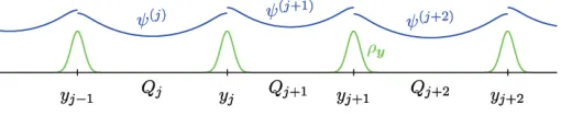
Fig. 4.1. The Cauchy–Born approximation: independent periodic problems are solved on the
cellsQj= (yj−1, yj)leading to locally defined fieldsψ(j).
to the full atomistic model and its stability. These results will enter the consistency and stability results on a/c couplings in sections 5 and 6.
Lety ∈ Y satisfy miny > ς0. The Cauchy–Born approximation is obtained by computing the energy of the cellsQj= (yj−1, yj) independently from one another, by treating each of them as part of a homogeneous chain (see Figure 4.1). We define the Cauchy–Born energy of the cellQj by
(4.1) Ejcb(y) =− min ψ∈H1#(Qj)
Qj
1
2ε2|∇ψ|2+12m2ψ2
dx−
Qj
ρyψdx
.
Note that this energy depends only on the distance (yj−yj−1). The minimizerψ(j) of (4.1) satisfies the equation −ε2Δψ(j)+m2ψ(j) =ρ
y in Qj and its |Qj|-periodic extension toR:
(4.2) −ε2Δψ(j)+m2ψ(j)=ρy(j) inR,
where we have defined the positionsy(j)= (yk(j))k∈Zof an infinite chain of equidistant atoms by
(4.3) y(kj)=yj+ (k−j)(yj−yj−1) ∀k∈Z.
The Cauchy–Born approximationEcb(y) of the atomistic energy E(y) is then given
by the sum over all cells
(4.4) Ecb(y) = N
j=−N Ecb
j (y) = 1 2
N
j=−N
Qj
ρyψ(j)dx.
In the Cauchy–Born model we seek to minimize the total potential energyEcb
f :Y →R
defined by
(4.5) Efcb(y) =Ecb(y) + (f,y)ε.
Whether the Cauchy–Born model is a good approximation to the exact atomistic model strongly depends on the regularity properties of minimizers of (4.5).
Letu∈ U be a test vector andu∈ S#(y) be an interpolant ofu; i.e.,u(yj) =uj forj∈Z. It follows as in Lemma 3.4 that the derivative ofEcb
j (y) can be written in the form
(4.6) DyEjcb(y)·u= uj−uj−1
yj−yj−1
Qj
σj,cby(x) dx=
Qj
where the local continuum stress functionσcb
j,y, in direct correspondence with (2.7), is
σcbj,y(x) = 12ε2|∇ψ(j)(x)|2−21m2ψ(j)(x)2+ρy(x)ψ(j)(x)
+ε
N
j=−N−1
ψ(j)(x)∇δε(x−yj)(x−yj). (4.7)
Furthermore, we define the Cauchy–Born stress functionσcb
y : Ω→Rby
σcby (x) =σcbj,y(x) if x∈Ωj
for allx∈Ω.
4.1. Consistency. Next, we turn to the consistency analysis of the Cauchy– Born approximation, for which we shall estimate the error of the Cauchy–Born forces in a norm suitable for the subsequent error analysis.
From (2.6) and (4.6) we deduce that
DE(y)−DEcb(y)·u≤
Ω
σy(x)−σycb(x)|∇u(x)|dx
= N
j=−N
Qj
σy(x)−σj,cby(x)|∇u(x)|dx,
where the stress functions σy andσcb
j,y are given by (2.7) and (4.7), respectively. To investigate the modeling errorσy(x)−σcb
j,y(x)incurred by going from the atomistic description to the Cauchy–Born approximation it is therefore sufficient to analyze |φ−ψ(j)|and|∇φ− ∇ψ(j)| inQj for everyj∈ {−N, . . . , N}.
Lemma 4.1. Let y∈ ∞(Z), and definey(j)= (y(j)
k )k∈Zby y
(j)
k =yj+εyj(k−j)
for allk∈Z; then,
yn−y(nj)≤(n−j)ε2y1([j,n−1]) for n > j,
yn−y(nj)≤(j−1−n)ε2y1([n+1,j−1]) for n < j−1.
Proof. Assume, without loss of generality, that n > j. Since yj−1 =y( j)
j−1 and
yj =y( j)
j ,
yn−yn(j)=ε n
k=j+1
yk −(yk(j))=ε2
n
k=j+1
k−1
l=j
yl−(y(lj))=ε2
n
k=j+1
k−1
l=j
yl,
where we have used that (y(j))is constant. Changing the order of summation we get
|yn−y(nj)| ≤ε2 n−1
l=j n
k=l+1
|yl|=ε2
n−1
l=j
(n−l)yl ≤(n−j)ε2y1([j,n−1]).
Lemma 4.2. Let y ∈ Y satisfy miny > ς0. Let φ ∈ H1
#(Ω) satisfy (2.2) and ψ(j)∈H1
#(Qj)satisfy (4.2), respectively. Then,
φ−ψ(j)L∞
(Qj)≤με ∞
n=1
y
1([j−n,j+n−1])ne−mnminy
,
ε∇φ−ε∇ψ(j)L∞
(Qj)≤mμε ∞
n=1
y
1([j−n,j+n−1])ne−mnminy
.
Proof. From Proposition 2.3 we immediately deduce that, for allx∈Qj,
φ(x) = 1 2m
R
k∈Z
δε(z−yk)e− m
ε|x−z|dz,
ψ(j)(x) = 1 2m
R
k∈Z
δε(z−y( j)
k )e− m
ε|x−z|dz. (4.8)
Sincey(jj)=yj andy( j)
j−1=yj−1, the respective terms in the sums cancel. Hence, we get forx∈Qj
φ(x)−ψ(j)(x) = 1 2m
k∈Z
k=j−1,j
R
δε(z−yk)−δε(z−y( j)
k )
e− m
ε|x−z|dz.
We now derive bounds on the individual terms in the sum. Note that (2.12) simplifies the following calculations, but due to the smoothness of the Green’s function similar bounds can be obtained without it.
Let k > j. Then we have |x−z| = z−x for all z ∈ suppδε(· −yk) and all
z∈suppδε(· −y( j)
k ). Thus, with (2.12),
(4.9) 1 2m
R
δε(z−yk)−δε(z−y( j)
k )
e− m
ε|x−z|dz= μ 2m
e− m
ε(yk−x)−e− m
ε(y
(j)
k −x).
Ifyk(j)≥yk, then
21m
R
δε(z−yk)−δε(z−yk(j))
e−mε|x−z|dz≤ μ
2me
−mε(yk−x)1−e−mε(y(kj)−yk)
≤ μ 2me
−mε(yk−x)m ε(y
(j)
k −yk).
Using (yk−x)≥(k−j)εminy for allx∈Qj and applying Lemma 4.1 leads to
μ
2εe
−mε(yk−x)y
k−y( j)
k ≤
με
2 y
1([j,k−1])(k−j)e−(k−j)mminy
.
The same bound on (4.9) can be obtained ifyk(j)≤yk.
For anyk < j−1 we can use the same techniques to obtain that
1 2m R
δε(z−yk)−δε(z−y( j)
k )
e− m
ε|x−z|dz
≤με 2 y
1([k+1,j−1])(j−k−1)e−(j−k−1)mminy
![Fig. 3.1. The atomistic model in the domain Ωa with Dirichlet boundary conditions g = [gL gR]T.](https://thumb-us.123doks.com/thumbv2/123dok_us/9584115.462185/10.612.125.386.104.159/fig-atomistic-model-domain-wa-dirichlet-boundary-conditions.webp)