(*) Notice:
Subject to any disclaimer, the term of this
(STCC, Ein Husch Blackwell LLP
patent is extended or adjusted under 35 ey, Agent,
U.S.C. 154(b) by 756 days.
(57) ABSTRACT
(21) Appl. No.: 12/297,179
Determining the structure of permanent charge for an ion (22) PCT Filed: Apr. 11, 2007 channel formulates an abstract operator, describing ion chan
nel parameters, comprising equations that are ill-posed. The p pr1S1ng eq p
(86). PCT No.: PCT/US2007/008976 model of ion channel behavior relates the function of the ion
S371 (c)(1) channel to the structure of permanent charge within the ion
(2), (4) Date: Mar. 16, 2009 channel and concentrations ions around the ion channel under certain properties and boundary conditions. The model also (87) PCT Pub. No.: WO2007/120728 includes regularization of the abstract operator by approxi mating the ill-posed equations with a family of well-posed PCT Pub. Date: Oct. 25, 2007 equations. An estimate of the closeness of the well-posed
O O solution to the ill-posed solution is provided. Providing stable
(65) Prior Publication Data and convergent algorithms allows the model to determine a US 2009/O253898A1 Oct. 8, 2009 stability for the regularized solution, so that a regularization
arameter can determine a balance between the stabilitv and
p y
Related U.S. Application Data accuracy of the Solution. (60) Provisional application No. 60/791,185, filed on Apr.
U.S. Patent
Dec. 18, 2012
Sheet 1 of 15
US 8,335,671 B2
FIG. 1
Forward start
> Forward solution
Design solution (- -
- - Design start
Identification solution <
-
Identification start
Structure of
permanent charge
{ (A, B, C), V
Current-voltage relation
for each of A, B, and C
Concentrations of
species present and
applied voltage
FIG 2
FIG. 3
Ca
15 M 10
s
o;
Ho
60 S5 50 45 40
s
30
25's O
Na'
2
M
5
1.
0.5
2 o; O 2
cy?
80 M
6d
40
20
2 O 2
x (nnn)
Algorithms
Program
0.8 0.6
0.4 C2
-2 2
Settric Polenia W
0.02 0.04
-0.6
0.08
U.S. Patent
Dec. 18, 2012
Sheet 3 of 15
US 8,335,671 B2
'total eror'
'' regularization error
---
--- '' propagated data error
- r
e.
-
c.
t 'ontinal regularization (arameter
FIG. 5
0.98
0.96 0.9. C.192
0.9
0.88 0.86 0.84 O. 182 .8
(). 178
O st too so 2O) 2s 300 350 40 as 500
FIG. 6
0.2
o s GG 50 2 250 300 350 40 45 50
Total oxygen Mass (Scated)
o o 2 So 60 50 S. 70 8s Sd 10
literation Number
FG. 8
U.S. Patent
Dec. 18, 2012
Sheet 5 Of 15
US 8,335,671 B2
x 10" east-Squares Functional
o o 3. 40 s s 8 s O
taration Nuer
x 10' east-Scuares functional
3.
s
2
s
*
a.
c 2 s 400 5 f s
0.32
03
0.3
0.
3
2S)
028:
27
0.28
s
24
22
c 20 So d 60 700 o 90 t
U.S. Patent
Dec. 18, 2012
Sheet 7 of 15
US 8,335,671 B2
Confining Potential
w).25 no.2 a). al. as 5. . 2 0.25
3.
Confinigotentif
0. s
-0.2
w3
f
1N
04
as
es
w8
w
0.2s a).2 0.5 es. ...ts 0.5 1. s 2 o,25
Confining Potential
-
: Reconstruction
'''''''' Exct
as -0.2 -0.15 -0, -0.05 0.5 O. 15 O.2 0.25
F.G. 12
U.S. Patent
Dec. 18, 2012
Sheet 9 Of 15
US 8,335,671 B2
east-Squares Frictional
0.22
e.
0.22.
122
o,
22
22
,02
0.22
o,022
testic ser
sef
2
3.
229
22
o, as a
terrtis Nkriter
Objective Functions and (negative) Penneability Ratio
O 2 4. S 8. 0. 2 14
U.S. Patent
Dec. 18, 2012
Sheet 11 of 15
US 8,335,671 B2
Exponential of Corfiiq Potential
.
-0,25. O2 a,15 -, -,9s Q.5 o, .S 2 2
Expo?ertial of Corfiring Potential
8 m
25 2.
22
2
B
s
ta 2
t
ods r0.2 -3 w). es
FIG. 5
s 8, is 02 0.2s
Objective Functional and (negative) Periteability Ratio
O OO 200 3. 40 50 soo 700 800 90.0 OO
eration fiber
FG 16
U.S. Patent
Dec. 18, 2012
Sheet 13 of 15
US 8,335,671 B2
Exponential of Confining Potential
6.25 -02 -O.S w). -5 OS O), 15 2 0.23
x 10' Exposertied of Corfiring Potential
O
2. a;2 , w). 0.0 0.5 0. 0. 0.25
FIG. 17
Selectivity Fier
f
/
f.
F.G. 18
L type Ca Channel
L type Ca Channel
s A so
Fied With Na
Fied With Ca
it to sco riot to scale
Cattle Prote is only cystics s . 4e
1) Glutamate Oxygens a de - See
2) i.E.h 2. Wolterne 0.38mm
3) Oielectric Constant 64 3) Dielectric Constant 64
Outside the Fter tie far
3 Solo 3kSalton
NaCl and Caci, NaCl and Caci,
F.G. 19
U.S. Patent
Dec. 18, 2012
Sheet 15 Of 15
US 8,335,671 B2
Piecewise constant functions, mss
FIG. 20
Piecewise linear functions, as
1. Field of the Invention
The present invention relates to methods for characterizing existing ion channels, and designing ion channels with greater specificity for predetermined ions.
2. Background Art
Ion channels are proteins that fold to form a hole down their middle. When properly configured and installed in a cell
membrane, ion channels control the movement of ions
through the cell membrane. An example of this transport would be the passage of Na', K, Ca", and Clions from the blood stream into and out of cells. The movement of ions into and out of a cell is very important for many processes that are critically related to health and disease in living things, includ ing people. Indeed, ion channels control an enormous range of life’s functions by controlling the flow of ions and elec tricity in and out of cells. A sample ion channel, 100, as illustrated in the prior art is provided in FIG. 1. The port exterior to the cell is labeled 102, and the port to the interior of the cell is labeled 104. The locations of the permanent charges that are the principal influences on how the ion chan nel conducts ions are labeled 106.
Ion channels conduct one type of ions much better than other types of ions, and this preference for conducting one type of ion over other types of ions into or out of a cell is termed “selectivity.” The selectivity of ion channels is a cru cial, indispensable part of their function.
If ion channels in living things lose their selectivity, activi ties critical to sustaining life cease. Thus, if the Ca" channels
of an animal or human heart were to become nonselective, or
become equally selective to Na' and Ca", the heart could not beat and death would occur in ~3 minutes.
Ion channels, like many other systems in biology are not perfectly formed; that is to say, they have characteristics which if changed could greatly increase their function. This characteristic of ion channels is particularly clear in the heart. A particular instance of this, the relevance of ion channels to the hearts of certain mammals is explained.
The heart is a sheet of cardiac muscle that is folded to enclose a ventricle, which is a cavity in the heart that holds the blood to be pumped. The ventricle has valves that operate to keep the blood flowing in one direction. The heart works by squeezing the blood out of the ventricle, say the left ventricle. The squeeze must start from the bottom of the ventricle (fur thest away from the exit valve and exit artery called the aorta). If the Squeeze starts anywhere else, contraction of the heart
muscle will be futile, the ventricle will not function as a
pump, and the animal or human will will quickly lose con sciousness and die. So coordination of the contraction of cardiac muscle is crucial for Survival.
In engineered systems of this sort, Such as artificial hearts,
and in the hearts of lower forms of life, coordination of this
sort is done by a control system that is separate from the
25 30 35 40 45 50 55 60 65
increased, the heart would be much less sensitive to this kind
of disruption. Thus limitations on the current flow through a calcium channel of the heart is one example of a technical deficiency of the heart. This is just one example. There are many others which physicians and pharmacologists discover every day, unfortunately.
The structures of ion channels are currently identified using X-ray crystallography to measure the positions of the key elements of the protein. Crystallography techniques have several shortcomings, not all of which are listed here. First, the crystallography is time consuming because it takes a long time to obtain a crystal Suitable for crystallographic study. Indeed, growing crystals is an art unto itself and most of the proteins of interest in membranes have not been crystallized. Second, proteins can fold differently in different environ ments. Therefore, even if the ion channel is crystallized, the protein as crystallized may not be in the same environment or state as it is in the animal as it functions. Thus, the crystal structure of the ion channel may not reflect the structure in the form in which it actually functions. Third, the X-ray crystal lography studies are only as good as the crystals provided, and take considerable time and resources. Whether the crystal was good enough to obtain the results desired is often not known until after the study is conducted. Fourth, the expertise needed to conduct the X-ray crystallography studies is Sufficiently different from the manufacture and design of the channels that it is rare for the same worker to be able to have the complete skill set, and thus workers in the field are dependent on the technical skills of a crystallographer.
The manufacture of ion channels is now sufficiently under stood such that if channels can be designed to specification they can be built using the well developed techniques of molecular engineering, e.g., by site directed mutagenesis. One example is given in U.S. Pat. No. 6,979,724 to to Lerman et al. which relates to calcium channel compositions and methods of making and using them. In particular, the Lerman disclosure relates to calcium channel alpha2delta (C26) Sub units and nucleic acid sequences encoding them. A review of ion channel manufacturing techniques is provided by 130. which should be available to the general public shortly. How ever, there are present shortcomings in the ability to under stand how the structure of an ion channel dictates its function Such that the technical ability to make an ion channel is not sufficient to solve problems in the field.
The technical limitations of present design methods are simple to state but hard to remedy. Generally, existing design methods rely on exhaustive trial and error experimentation of the highest quality, energy, and imagination to check reason able guesses. This approach to design is inefficient and rarely works in complex systems.
US 8,335,671 B2
3
of this work is done without theoretical guidance, or rationale, using the trial and error methods of exploration and discovery of traditional biology. Such trial and error methods are essen tial for learning “the lay of the land’, for describing the systems and their components, but they are very inefficient for design. If it was possible to replace trial and error methods with any systematic design tool, the efficiency of thousands of laboratories would be dramatically increased, from nearly Zero (which is the efficiency when design is unsuccessful) to a reasonable number.
More recent attempts at design have used simulations of atomic motions, calculations of the movement of every atom of a protein. Such calculations, despite heroic efforts and enormous computers, are unlikely to Succeed because bio logical function occurs on millisecond time scales or slower, and atomic motions occur on 0.0000000000000005 sec time scales (femto seconds and faster). Biological function occurs (in many cases, e.g., in the channels of the heart) only when certain chemicals are present in definite concentrations. Some of these chemicals must be present in micromolar con
centration. Thus, atomic scale simulations of these chemicals
must include enormous numbers of atoms for many seconds, with motions on the time scale of a femtosecond being
resolved. Thus, at this time, atomic scale simulations serve as
metaphors and inspiration for design, but not as specific quan titative design methods. While there have been some attempts to use reduced models of channel function that do not include all atomic motions, they have not succeeded in designing a channel of a desired selectivity or in discovering the structure of an ion channel from data taken from the operation of a channel in vivo or in vitro.
Presently, the design theory of ion channels generally ana lyzes ion channels by linking a model for the electric field in and near the ion channel with a model for ion transportin and near the channel. Generally, such studies are currently con ducted using what are termed "one dimensional models.” which model an ion channel as a line with charges placed along it in fixed locations. These placed charges are often referred to as “fixed charge” or “stationary charge' to distin guish these charges from the charges of the ions that are moving around and through the channel. The most commonly used models for the ion transport in the vicinity of the channel are built from either the Poisson-Boltzman equations or the Poisson-Nernst-Planck (PNP) equations. Other models used
include, but are not limited to, simulations of Brownian
motion, simulations of Brownian motion with Poisson equa tion, and transport Monte Carlo. Viewed in terms of physical chemistry, the models attempt to describe energetics of anion moving through an ion channel. Viewed mathematically, these equations form what is called a system of non-linear differential equations.
In searching for ion channels with a particular selectivity, different approaches can be taken. One way of Solving the selectivity problem would be to hypothesize an ion channel and ask how it might perform for different ions. Efforts to design ion channels by Solving ensembles of possible ion channels in the hope of finding Suitable structures have not been productive, as illustrated by references 93-128.
The ion channel Scientists have yet to predetermine a par ticular selectivity for an ion channel, and then Successfully attempt to determine what a channel that would have that selectivity would look like. Many kinds of scientists under stand that problems can often be viewed or approached in
10 15 25 30 35 40 45 50 55 60 4
and wish to predict what will happen, or one may be observ ing effects and wish to infer the cause.
When searching for causes of observed or desired effects the problems are termed “inverse problems” which are likely to be difficult to solve. Two problems are called inverse to each other if the formulation of one problem involves the solution of the other one. These two problems then are sepa rated into a direct problem and an inverse problem. At first sight, it might seem arbitrary which of these problems is called the direct and which one the inverse problem but this arbitrariness is more apparent than real. The problems have quite distinct properties and can be distinguished based on those properties.
Usually, the direct problem is the more “classical' one, in that it usually has a single, obtainable solution, which is termed “well-posed. According to Hadamard, a mathemati cal problem is called well-posed if
for all admissible data, a solution exists,
for all admissible data, the Solution is unique, and the solution depends continuously on the data.
Much of the mathematical theory of partial differential equa tion deals with the question what “admissible data” means and in which sense “solution' is to be understood for specific classes of partial differential equations.
The direct problem usually is to predict the evolution of the studied system (described e.g. by a partial differential equa tion) from knowledge of its present state and the governing physical laws including information on all physically relevant parameters including boundary conditions and initial condi tions. Boundary conditions are parameters that describe the behavior of the physical system or set of equations at the edges of a simulation region. Conditions imposed at the start ing time for a problem where the conditions change over time are called initial conditions.
Those of ordinary skill in the art will appreciate that bound ary conditions and initial conditions are much more important than they may seem at first to the uninitiated. Boundary con ditions and initial conditions describe what is put into the system and what comes out of it. They describe the flow of energy, matter, electric charge, et cetera that are forced to enter and leave the system. Boundary conditions are fully as important as the system itselfin determining the overall prop erties of a practical system. Indeed, there are many engineer ing systems that are designed to have specific inputs and outputs (i.e., initial and boundary conditions) only. That is to say, there are many engineering systems designed so the user does not need to be concerned what is inside the “blackbox' (i.e., inside the system) but only needs to be concerned with the inputs and outputs (i.e., boundary and initial conditions). Thus, in electronics, a well designed amplifier has a simple relation between input and output (called gain) and the user does not have to worry if the amplifier uses field effect tran sistors, bipolar transistors, or even old fashioned tubes to make that gain.
modeling errors or other, even numerical, inaccuracies. The process of bringing stability back to these problems is termed regularization. Often, regularization is done by imbedding an ill-posed problem into a collection of well posed problems depending on Some parameter, where the original ill-posed problem is a limiting case of this family of well-posed problems with respect to this parameter.
Non-uniqueness is sometimes an advantage, because non uniqueness can allow a choice among several strategies all of which achieve a desired effect. The non-uniqueness of the Solution can be advantageous because one strategy might have better properties than another. When solving design problems there is a Substantial value to having a choice of solutions because that allows the problem solver to choose from different possible designs based on practical advantages not included in the mathematical model itself. This is in contrast to an identification problem where having a choice of solutions means that the identification is ambiguous.
In the case of designing ion channels it is advantageous to look for values of parameters (possibly fulfilling additional constraints) that achieve certain design goals (like selectivity in ion channel design). In contrast, in an identification prob lem, one wants to infer (identify) values of parameters from indirect measurements, i.e., parameters are estimated not from direct measurements of the parameters but from mea surements of other quantities from which estimates of the parameters are made. These other quantities appear in the mathematics as quantities in the output of the forward prob lem (and its boundary conditions). The inverse problem is used to estimate these parameters from measurements of the output under some conditions or other, or from multiple mea Surements of the output under a set of conditions (to give more information and reduce sensitivity to, for example, mistakes and noise). Here, in Solving this inverse problem, uniqueness (“identifiability') is of great importance.
Uniqueness questions are dealt with explicitly in one part of the mathematical literature of inverse problems, but as Soon as one wants to compute solutions of inverse problems, one almost always has to deal with the issue of (in)stability: In practical applications, one never has exact data, but only data perturbed by noise produced by Systematic or statistical errors in the measurements or produced by errors in the math ematical model itself. Models are often only a representation of reality with limited accuracy. Even if the random and/or systematic deviation from the data is small, or the error in the model is small, algorithms developed for well-posed prob lems will fail if they do not address the instability in the overall process of estimation of parameters. If they do not address the instability of the inverse problem due to a viola
tion of the third Hadamard condition, data as well as round
off errors can then be amplified by an arbitrarily large factor (depending on error characteristics) arising from this lack of continuous dependence, the violation of the third Hadamard
25 30 35 40 45 50 55 60 65 Radon transform.
Inverse scattering (cf. 17, 65), where one wants to reconstruct an obstacle oran inhomogeneity from waves scat tered by those. This is a special case of shape reconstruction and closely connected to shape optimization 41: while in the latter, one wants to construct a shape such that some outcome is optimized, i.e., one wants to reach a desired effect, in the former, one wants to determine a shape from measurements, i.e., one is looking for the cause for an observed effect. Here, uniqueness is a basic question, since one wants to know if the shape (or anything else in some other kind of inverse prob lem) can be determined uniquely from the data (“identifiabil ity'), while in a (shape) optimization problem, it might even be advantageous if one has several possibilities to reach the desired aim, so that one does not care about uniqueness there. Inverse heat conduction problems like Solving a heat equa tion backwards in time or "sideways” (i.e., with Cauchy data on a part of the boundary) (cf. 30).
Geophysical inverse problems like determining a spatially varying density distribution in the earth from gravity mea surements (cf. 27).
Inverse problems in imaging like deblurring and denoising (cf. 14, 55, 60])
Identification of parameters in (partial) differential equa tions from interior or boundary measurements of the Solution (cf. 3, 46), the latter case appearing e.g., in impedance tomography (cf. 45). If the parameter is piecewise constant and one is mainly interested in the location where it jumps, this can also be interpreted as a shape reconstruction problem. Some common features of inverse problems that provide technical Solutions to technical problems are problems such as amplification of high-frequency errors, a need to use one or both of a priori information and regularization to restore stability, errors of differing natures that require separate treat ment, and intrinsic information loss even if one does every thing in the mathematically best way. Examples of errors requiring different treatment are errors of approximation, which are how closely the model is hewing to the actual system, and the propagation of data error, wherein errors in earlier calculations cause greater errors in later calculations. Detailed references for these and many more classes of inverse problems can be found e.g., in 23, 20, 22., 37. 53, 50, 44, 16. In order to overcome these instabilities and design solution techniques for inverse problems which are robust (i.e., stable with respect to data and numerical errors), one has to design and use regularization methods, which in general terms replace an ill-posed problem by a family of neighboring well-posed problems.
US 8,335,671 B2
7
use trial and error approaches that require solving ensembles of possible ion channels in the hope offortuitously finding the desired result. This would be especially advantageous where existing ion channels are less than optimal for the function that they perform. This would be of greatest importance if the technology were able to characterize and design the selectiv ity of ion channel functions that are important to the life and health of animals, including humans.
Further, if the methods could pioneer the identification and design of selectivity through in vitro and in vivo experiments, the technical horizons of laboratory work in the field would be significantly broadened accelerating not only design, but also manufacture and testing. Similarly, if the technology that solved the problems of the identification of structure and design of selectivity could be applied to a broad range of models, the ability of theoretical workers to contribute to the Solution of existing technical shortcomings of existing ion channels would be similarly amplified.
BRIEF SUMMARY OF THE INVENTION
A model for determining a structure of permanent charge for an ion channel from information formulates an abstract operator describing ion channel parameters comprising equa tions that are ill-posed for determining the structure of per manent charge of an ion channel. The model of ion channel behavior relates the function of the ion channel to the struc ture of permanent charge within the ion channel and the concentrations of ion species present in the region in and adjacent to the ion channel given that certain properties and boundary conditions are known. The model also includes the regularization of the abstract operator by approximating the equations that are ill-posed for determining the structure of permanent charge of an ion channel with a family of well posed equations to provide a regularized solution of ion chan nel parameters. An estimate of the closeness of the regular ized solution to the solution is provided via the abstract operator to obtain an accuracy of the regularized solution. Providing stable and convergent algorithms allows the model to determine a stability for the regularized solution, so that when at least one regularization parameter is provided, the regularization parameter can determine a balance between the stability stability of the regularized solution and the accu racy of the regularized solution.
In one embodiment of the invention, formulating the abstract operator includes providing a forward model of ion channel behavior, information regarding the structure of per manent charge for a control ion channel, and a plurality of sets of mobile species concentration information, where a set of mobile species concentration information comprising a con centration of the first mobile species and a concentration of the second mobile species. Then, a corresponding ensemble of data for the relationship of current to voltage for the control ion channel can be provided for each of the plurality of sets of mobile species concentration information. The forward model of ion channel behavior can then be solved for the control ion channel based on the mobile species concentra tions and the relationship of current to Voltage.
In another embodiment of the invention, the forward model
of ion channel behavior for the control ion channel further can be solved by providing a fast and accurate algorithm for the forward mode, and providing an accuracy for the forward model.
In another aspect of the invention, a structure of permanent
5 10 15 25 30 35 40 45 50 55 60 8
determining the structure of permanent charge as previously mentioned is provided, then control data comprising control permanent charge data, control mobile species data, control applied Voltage data, and control current-Voltage relationship data can also be provided. This allows the model for deter mining the structure of permanent charge to be applied to the control data.
In an exemplary embodiment of the present invention, the ion channel model is a Poisson-Planck-Nernst model. In another exemplary model of the present invention, regulariz ing the abstract operatoruses regularization methods from the group consisting of variational and iterative approaches. One application of the invention is to design a structure that includes a selectivity of the ion channel between at least a first
mobile ion and a second mobile ion, and the structure is
determined from the selectivity. Optionally, a structure is identified based on indirect data that is experimental data derived from measuring an actual ion channel. Alternatively, an ion channel can be constructed according to a design created by the methods described.
The invention further contemplates using an ion channel according to the disclosed methods, such that the ion channel has a first opening and a second opening, and the ion channel
is installed in a membrane, such that if the membrane has a
predetermined electrical potential across the membrane, the ion channel will select, relatively, for the transport of the first mobile ion species relative to the transport of the second mobile ion species.
In another aspect of the present invention, the model for determining the structure of permanent charge includes deter mining the manufacturability of a the determined structure of permanent charge for the ion channel from the structure of a pre-existing ion channel. This can be done by providing the structure of a pre-existing ion channel; and applying the model to the structure of the pre-existing ion channel. This alternatively includes constructing an ion channel for a pre determined function by designing an ion channel Suitable for carrying out the predetermined function using the methods described, and constructing an ion channel that approxi mately embodies the ion channel designed for carrying out the predetermined function.
One benefit of the present invention is that workers in the field will be able to control the structure and selectivity of ion channels, and be able to reliably design ion channels with specifically predetermined selectivity. More beneficially, Such methods would not use approaches that require solving ensembles of possible ion channels in the hope offortuitously finding the desired result. The invention is especially advan tageous where existing ion channels are less than optimal for the function that they perform. This would be of greatest benefit in areas where the ability to characterize and design the selectivity of ion channel functions that are important to the life and health of animals, including humans.
error data combine to provide an estimate of total error. FIG. 6 is a plot of the data propagation error term versus k—this term will go to infinity ask goes to infinity.
FIG. 7 is a plot of the regularization error term versus k—this term will go to 0 ask goes to infinity.
FIG. 8 is a plot of the total charge (relative to the exact value) during the iterations of the gradient method.
FIG. 9 is a plot of the squared residual ||F(P)-III as a
function of the iteration number for 4x2x2 measurements (above) and 6x3x3 measurements (below).
FIG. 10 is a plot of the identification error ||P-P-II as a
function of the iteration number for 4x2x2 measurements (above) and 6x3x3 measurements (below).
FIG. 11 are the final reconstructions P* obtained at the stopping index determined by the discrepancy principle for 4x2x2 measurements (above) and 6x3x3 measurements (be low).
FIG. 12 shows the initial value Po used for all reconstruc tions of potentials.
FIG. 13 is a plot of the residual (above) and identification
error ||P-P-II (below) as a function of the iteration number
without regularizing stopping criterion.
FIG. 14 shows the objective functional J(P) for C.200 and negative permeability ratio as a function of the iteration number.
FIG. 15 shows the initial value (above) and computed optimal potential (below) for the functional J with C.200.
FIG. 16 shows the objective functional J(P) equal to the negative permeability ratio as a function of the iteration num ber.
FIG. 17 shows the initial value (above) and computed optimal potential (below) for the functional J.
FIG. 18 illustrates the relationship of the permanent charge region to the ion channel as a whole.
FIG. 19 illustrates the positioning of possible ions in an example permanent charge region of an ion channel.
FIG. 20 illustrates an application of piecewise constant functions which are constant within an interval to model the electrical potential and flux region by region.
FIG. 21 illustrates an application of ramped linear func tions that form a continuous series of ramps to model the electrical potential and flux region by region.
DETAILED DESCRIPTION OF THE INVENTION
1. Introduction
For the purposes of the present disclosure, solving the forward problem derives a current-voltage relationship from a predetermined structure of permanent charge (synonymous with “fixed charge') and predetermined concentrations of mobile species, and the electrical potential (sometimes referred to as “voltage') across the ion channel.
25 30 35 40 45 50 55 60 65
charges distributed along an X-axis, defines the locations of charge in a one-dimensional space. The concentrations of mobile species, 204, define the concentrations of different mobile species to be modeled, and constitute inputs to both the forward and inverse problems, along with V. applied volt age. Generally, this will include the solvent, the ions to be selected for and against, and counterions for the ions that are Subject to selection or non-selection. The current-voltage relationship, 206, describes the line, or set, of relationships that describe how many ions move through the channel at a particular voltage. It should be noted that for each structure of permanent charge, there are infinite ensembles of relation ships between the ion concentration and applied Voltage inputs and the Voltage-current relationships.
The structure of permanent charge, 202, is the electrical structure of the system. Like any structure it provides the framework for what a system can do but it does not tell what the system does until driving forces and control signals are applied to the system. Think of a car. The structure of the car tells a lot about the car and knowledge of the structure is necessary to understand and improve the car. But the car does not move unless gasoline is in the tank, water in the radiator, lubricants and oils in the right places (etc), and the car does not move until a control signal is given telling it to move. The automobile needs driving forces (the gasoline), Supporting items (water and oil), and a control signal too. Ion channels are similar. They need driving forces. The driving forces for ion flow through channels are the concentrations of ions outside the channel and the electrical Voltage across the chan nel. The supporting forces are the dielectric properties of the lipid membrane and various biochemicals. The control signal is different for different types of channels. In some it is a specific chemical; in others it is pressure; in others the control signal is Voltage. Thus, we see that the properties of any channel structure correspond to a multitude of ensembles of properties of current voltage curves. Each different driving force gives a different current voltage curve. Each different biochemical or dielectric property gives a different current Voltage curve. Each chemical or pressure gives a different current Voltage curve. And each driving force at each pressure gives a different current voltage curve. Thus, the number of current Voltage curves is as large and disparate as the number of trips a car can take. The car has only one structure but it can go many places in many different ways.
US 8,335,671 B2
11
Thus, each current Voltage curve can be described adequately by a complicated polynomial equation with 5 parameters or thereabouts. The current Voltage curves are generally studied from the smallest detectable currents, say 0.1 p.A, to the largest allowable applied voltage which is typically 150 mV. No time dependence is involved when only open channels are studied. Open channel currents are independent of time from approximately 1 usec to the longest times that can be studied, e.g., seconds. Current Voltage curves vary depending on the ions present to carry current. Thus current Voltage curves are typically measured first in a “pure' systems consisting of one electrolyte (like NaCl) on one side of the channel and the same electrolyte on the other side of the channel. Measure ments are then made for a series of different concentrations. First, the concentrations are the same on both sides, so typi cally measurements would be made at 20 mM, 50 mM, 100
mM, 500 mM, 1 M, 2 MNaCl. Then different concentrations
would be used on the two sides, with all combinations being explored, e.g., 20 mMonone side with 50 mM, 100 mM, 500
mM, 1 M, 2 MNaCl on the other. Lower concentrations than
20 mM would be avoided because they tend to damage the channel protein. Then the ion would be changed. Typically,
Li", Na', K", Rb", and Cs" would be studied. Then mixtures
of ions would be studied, starting with two at a time, e.g., NaCl and KCl mixtures on both sides of the channel but at different concentrations (in most cases). Work would then be done on divalent ions. Here concentrations would often be much lower because biological channels work better in low divalent concentrations. Typical ions would be Ca' and Ba'" but others are often used as well. Current can be carried by hydrogen ions and hydronium ions so pH is often varied as well. Finally, 'exotic organic cations like choline or tetram ethylammonium are often used as well as less exotic organic anions like amino acids.
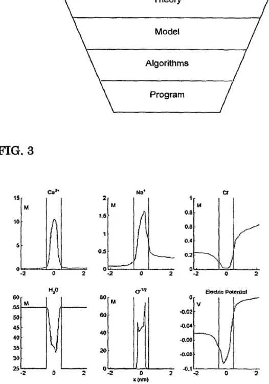
In the middle of FIG. 2 is a box that represents the physics that relates the structure of permanent charge, mobile species and applied Voltage inputs, and the current-Voltage-relation ship to each other. In describing the physics of ion channels, how the structure of permanent charge of an ion channel relates to the current-Voltage relationship as a function of mobile species concentrations and for the purposes of the present discussion is embodied in a function F, which, in an abstract sense, symbolizes how structure is transformed into the observable or desired output. Referring to FIG.3, F can be described on a variety of levels, with a variety of resolutions. At the highest level is the theoretical physics or chemistry selected for describing the interactions of the parts. However, in order to solve the problem a more concrete level of descrip tion is needed that necessarily imposes some degree of approximation in order to create a model to describe F. A model is a set of equations that are selected to concretely describe the interactions indicated by the theoretical physics and chemistry. Before the model can be implemented com putationally, a set of algorithms is selected in order to make a solution computable, and preferably, efficiently computable. Making the solution computable or efficiently computable will usually require yet another level of approximation. Last, the model as implemented with the selected algorithms is embodied in computer code so that a result can be obtained from a computer having a processor to execute the calcula tions and a memory to store inputs and outputs for the pro cessor. The result may be used in any way that is common for computer implemented Solutions, for example by displaying the result (such as on a monitor or projector), saving the result
10 15 25 30 35 40 45 50 55 60 12
networks, or modem, serial or other connection). The choice and design of algorithms may involve approximations so the problem will fit in the available memory and run with reason able speed on the processors available. Each aspect of this invention should be understood to be operable at all of these levels, from the most abstract to the useful, tangible and concrete results.
Mathematically, the present approach for identifying and designing ion channels formulates the inverse solution of permanent charge as an abstract operator equation or optimi zation problem involving models for the flow of electrical charge through the channel. The abstract operator equation is ill-posed and can be regularized (used in the most general sense) using several methods, exemplarily in this disclosure by using iterative methods with appropriate stopping crite rion. Alternatively, or in addition, the abstract operator equa tion can be regularized by using an additional penalization of the objective functional in the formulation as optimization problem, in order to be able to solve the problem numerically in an efficient, stable and robust way. Because the inverse problems are ill-posed in the sense that small differences in the electrical current can correspond to large differences in the permanent charge, regularization is necessary. In the con text of identification, the regularization methods are desirable to allow one to compute a stable approximation of the real permanent charge in the channel. In the context of design, regularization methods are desirable so one can introduce a-priori ideas of Suitable designs, such as attempting to con form Suitable designs to being easily engineered variations of existing designs.
This disclosure describes, among other things, how to per form ion channel design and identification. First, a class of models is used that is believed to reasonably describe the function of ion channels if all of the parameters and boundary conditions are known. Second, a class of algorithms that can be used to efficiently and stably solve the related “inverse problem” is described. Finally, the disclosure shows by examples that these methods succeed in both the tasks of identification and design. While the steps of solving the prob lem are described from beginning to end, those of ordinary skill in the art will appreciate that each of the steps influences the others, and that the solution to this class of problems, and the example in particular, may be performed partly or wholly out of the listed order. As will be appreciated by those of ordinary skill in the art, or have studied the field of applied
mathematics, much of the education of an advanced under
graduate or graduate student in applied mathematics is devoted to teaching how the steps influence each other, and how to vary the order of the particular steps of the solution.
The first class of models that describe the function of ion channels is termed here the “direct problem” or “forward problem.” This includes selecting interactions to describe the physical system, mathematically describing those interac tions in a model or models, selecting computational schemes or algorithms to implement the models, and then program ming the necessary computer code, with its attendant limita
tions, to reach a result.
2. Modeling Ion Channels
Models for ion transport through channels presently incor porate the following effects:
sional ion channel is an approximation that reduces the com putational complexity and hence computation time for solv ing the model. However, at the expense of significantly complicating the computations, the one-dimensional model can be replaced by those of ordinary skill in the art with
two-dimensional or three-dimensional models, and the
present invention is not limited to one-dimensional models, or even any particular one-dimensional model. Indeed, students and postdoctoral fellows in molecular biophysics and com putational biology learn to Switch between one, two and three dimensional models to choose what is needed to solve the particular problem at hand with available computational
SOUCS.
Further, in the exemplary embodiments, models for vari ous physical aspects of the systems such as electric field orion transport are used. The models selected are believed to be the best approach to solving problems of this sort at this time, but other models could be used to model the various physical behaviors in this invention. Accordingly, the present inven tion should not be considered to be limited to particular mod els for the systems analyzed.
Turning to the definition of the class of models that are the forward problem, a first model is selected to describe the
electric field, and a second model is selected to describe the
diffusion of ions in the region of the ion channel. These two models interact with each other. In the exemplary embodi ment of the present invention the model for the electric field is a Poisson equation with a source term equal to the charge generated by the ions. Also in the present exemplary embodi ment, differential equations are usually used to describe the continuum description of ion transport, in particular the so called Nernst-Planck (NP) equations, which are an applica tion of the usual laws of diffusion (Fick's laws) to charged particles like ions. The solutions of the Nernst-Planck equa tions are the number densities of ions expressed as functions of their spatial location, in the channel and Surrounding baths. The Nernst-Planck equations can involve a diffusion term, a drift term caused by the electric field (ideal electrostatic potential), by an external constraining potential, and by the excess electro-chemical potential. Alternative models for the electric field could be Coulomb's law applied to all charges in the system, Coulomb’s law applied to periodic boundary conditions, Coulomb's law with Ewald sums applied to peri odic boundary conditions, Particle-Particle-Particle Mesh, Particle-Particle-Particle Mesh with double counting correc tions. Alternative models for the description of ion transport could be Brownian dynamics, Langevin dynamics, molecular dynamics, Transport Monte Carlo, and barrier models.
When the Poisson equation and the Nernst-Planck equa tions are used together to create a model, the coupled system for electric field and ion densities is then commonly called a Poisson-Nernst-Planck (PNP) model. At equilibrium, the
25
30
35
40
45
50
55
60
65
learning how to apply well established methods to different models.
The PNP model can be set forth as follows. Though there are many known variations of the PNP modeling approach, the present invention is not limited to a particular model of the interactions. In a computational domain S2 modeling the bath and ion channel region, the general structure of the model for describing the unconstrained electrical behavior of the mobile species of interest is of the form of the linked equa tions:
-AAV =X3 p.
(1)
k
-V (pi Valia, ... , p.m., VI) = 0 (2)
where V is the electric potential, p denotes the density of mobile species k with charge Z and mobility m. W is a dimensionless parameter whose size is inversely proportional to the scaling of the permanent charge in the channel. In particular, for a large permanent charge relative to the scaling to the system size one can expect w to be small, and hence equation (1) becomes a singularly perturbed Poisson equa tion, which creates various mathematical and computational complications. The complications include, but are not limited to different forms of the solution, multiple values of the Solution, computational difficulties arising from the singular or nearly singular form of the problem, and other problems characteristic of singularly perturbed systems of partial dif ferential equations as will be well known to those of ordinary skill in the art of Solving singularly perturbed non-linear differential equations.
The potential L is the functional variation of energy func tional E with respect to the density p i.e.,
3
= - EA1, ... Öpk , OM, V) W. (3)
k
The Poisson equation (1) is an equilibrium condition for the energy functional, i.e.,
O = av Ip1, ... , p M. V. E V (4)
US 8,335,671 B2
15
charge which fact is evident from the Nernst-Planck equa tion (2), which does not enforce equilibrium of the ions (1-0) in general, but only for special boundary values such thatu-0 on CS2. Ion channels do not function at equilibrium and so equilibrium analysis alone is not sufficient.
The energy functional can be written in the form
E?p,..., p. V7 (-).VY^+z Yp+Dp log
p-t|lp)dx+Ep1, ..., p. (5)
with D denoting a diffusion coefficient, E denoting the
excess electro-chemical energy and u" denoting the external
constraining potential acting on mobile species k. Those of ordinary skill in the art will appreciate that the energy func
tional could be written in other forms, and that while the
present invention is exemplified by this energy functional, it is not limited to this form of the energy functional. The energy functional is a subject of active investigation in the field of statistical mechanics of simple and complex fluids. Some forms of it are given in the Mean Spherical Approximation and Hypernetted Chain Theories, others in various versions of Rosenfeld’s Density Functional theory, including those opti mized to include electrical potential, and in the White Bear Functional.
The system defined this way is coupled to a constitutive model showing how the potentials arise from the structure and physics of the channel. Again, while the invention is exemplified by a particular model, it is not limited to the particular model. The excess electrochemical potentials (ob tained as variations of the excess free energy with respect to the particle densities) describe the direct interactions between the ions, and are usually obtained from hard-sphere models or Lennard-Jones potentials. The external constraining potential describes the external forces on the ions due to the structure and chemical nature of the channel. The external constraining potential is of particular relevance for the ions creating the permanent charge of the channel because the external con straining potential determines the confinement to the selec tivity filter, thereby having a large effect on the selectivity of the channel.
In the exemplary embodiment, a specific model based on density-functional theory (DFT) and mean-spherical approximations (MSA), as described in 34, 35, 59 is used, but as will be appreciated by those of ordinary skill in the art, the treatment of other models for excess electro-chemical potentials can be carried out with similar computational schemes and leads to the same kind of inverse problems as described below. Graduate students and postdoctoral fellows in statistical mechanics of simple and complex fluids are ordinarily trained in the skill of constructing and using similar models.
The standard computational schemes for PNP-systems can be based on an iterative (sequential) decoupling of Poisson and Nernst-Planck equations (Gummel-type methods) or coupled Newton-iterations. See references (77-91. The disadvantage of Gummel-type iterations is a non-robustness with respect to certain parameters in the selected model, in particular Vandu. Newton-type methods are more robust, but still the (non-symmetric) linearized problem to be solved in each iteration step is not well-posed for large parameters.
Moreover, as usual for Newton methods, one needs additional
globalization techniques.
The present disclosure presents an approach based on a symmetric linearization of the problem, which is motivated by the energy minimization approach used in equilibrium
10 15 25 30 35 40 45 50 55 60 16
trated here permits a so-called mixed finite element approxi mation, i.e., where the densities are approximated by discontinuous functions (e.g., piecewise continuous ones) across a partition of the domain (into Subintervals in one dimension), and the fluxes J. Zmp All are approximated by continuous functions (e.g., piecewise linear ones). While those of ordinary skill in the art of solving differential equa tions are familiar with mixed finite element approximations, those workers from other fields seeking information can find an adequate references in 129.
For the electric potential V a standard finite element dis cretization with continuous Ansatz functions (e.g., piecewise linear) can be used, because the gradient of V also appears in the energy functional. With this discretization, an iterative scheme is obtained, where a symmetric linear system has to be solved in each step, with the unknowns being the coeffi cients of the finite element basis functions.
With standard finite element discretization with continu ous Anzatz, functions and computations of the excess electro chemical potential as in 34, an iterative scheme based on the Solution of symmetric linear systems in each iteration step is constructed. The iteration constructs a sequence (p". . . . . p", V') and additionally fluxes (J". . . . . J.") by Solving coupled linear systems of the form
A°AV+X 3. p = 0
(6)
k
st-ve, -u
n, (p;-p;) - V. J. (8)
or more precisely their mixed finite element discretizations. Here m20 is a damping parameter that can be adapted to
obtain global convergence, and u?" is a linear approximation
of Lip". . . . . p'V' (linear with respect to the sequence
p". . . . . p", V*). It turns out that this scheme is not only
robust with respect to the major parameters, but even leads to decreasing iteration numbers with decreasing Debye length W, which is an important feature since the scaling of most interesting systems yields a small value of this parameter. As disclosed below, the solution of inverse problems will force the forward problem to be solved a very large number of times, so that efficiency in the computational methods for the forward problems is crucial.
To solve the forward problem, data about a particular ionis needed. The solution of the forward model for an L-type Ca-channel (described in detail in 34) is illustrated in FIG. 4. The data from 34 is used to provide values for the param eters identified by fixing the locations of the fixed or perma nent charges. In this channel, there are three mobile ion spe cies, Ca", Na", Cl, a neutral mobile species H2O, and one confined species (the permanent charge species), namely
half-charged oxygens O'. Half charged oxygens are typi
by the external constraining potential, which is represented
by u" (with k being the index of the oxygens), the shape of the
oxygen density inside the channel is determined by this
potential, the total number N=8 of the O'oxygens, as well
as the interactions with the other species. The inverse prob lems discussed in the following section will deal with the determination of the properties of the permanent charge, i.e., the oxygens in this example:
3. Regularization Methods for Nonlinear Inverse Problems
As those of ordinary skill in the art will appreciate, usually the mathematically most efficient way to formulate inverse problems involving partial differential equations uses con cepts and methods from functional analysis. Nonlinear inverse problems can then be cast into the abstract framework of nonlinear operator equations
where the operator Facts between two function (e.g., Hilbert) spaces X and Y. The basic assumptions for a reasonable theory are that F is continuous and is weakly sequentially closed, i.e., for any sequence X, CD(F), X, eX weakly in X and F(x)->y weakly in Y imply that x6D and F(x)=y. (cf.
23, 24). As opposed to the linear case, F is usually not explicitly given, but represents the operator describing the direct (also sometimes called “forward') problem. For example, for the ion channel model described previously, F would be the operator F mapping the constraining potential Lt. (with being the index corresponding to the permanent charge) into the outflow current used later to describe the inverse problem of identifying the constraining potential related to the permanent charge. Thus, computing a value of the operator F for a given input x involves solving the problem (1), (2), which is quite a difficult task. The values of a deriva tive of For values of an approximation to the derivative need to be computed, which involves solving a linearized partial differential equation. These computations appear in Solution methods for inverse problems several, possibly many, times, so that efficient solution techniques for the direct problemand for its linearizations have to be found and efficiently coupled with solution strategies for the inverse problem.
As a relatively simple example (not related directly to the ion channel problem) to illustrate this point (and also to illustrate a specific algorithm below), we use the following model problem. The problem, in its one-dimensional version described further down, describes the heat and temperature in a bar of material that is kept cold at either end, but may be heated in the middle:
The temperature u (as a function of location after suffi ciently long time, i.e., in equilibrium) of a conducting mate
25
30
35
40
45
50
55
60
65
Note that (10) with unknown q is nonlinear, because the relation between this parameter and the Solution u—that serves as the data in the inverse problem is nonlinear even if the direct problem of computingu with given q is linear. For this parameter identification problem, the parameter-to-out
put map F maps the parameter q onto the solution u, of the
state equation (10) or to the heat flux
dit
4,
Thus, computing F(q) means to (numerically) solving (10) with the parameter value q. We will come back to this model problem later.
Neither existence nor uniqueness of a solution to (9) is guaranteed for the problem posed in (10). Assuming for the sake of simplicity that the exact data y are possible (i.e. attainable)—i.e., that (9) in fact has a solution and that the underlying model is thus correct we use a generalized solu tion concept (see 4 for the general, non-attainable, case):
For x*eX, we call a solution x of (9) which minimizes
Ix-X among all solutions an X-minimum-norm solution of (9) (x*-MNS for short). The element X* can and should include available a priori information like positions of singu larities in X if they happen to be available.
One main issue in Solving an inverse problem (9) is that its Solution or solutions do not depend continuously on the data y. This can be seen easily if one considers the one-dimen sional version of (10). The one-dimensional version of (10) is
This can be solved explicitly:
For S e 0, 1: (-gu')(s) = I findi
O
the parameter q in terms of U is obtained via
I findi
OU(s)
US 8,335,671 B2
19
also in q. In addition, where the temperature gradient U" is close to Zero, errors in the Source term fand in the integration are heavily amplified since U"-0 is in the denominator of equation.
That issue implies that standard methods cannot solve problems like (9) with discontinuous dependence on data. For the inverse ion channel problem, we will show the discon tinuous dependence on data below in examples in Section 5.3. Thus, methods have to be developed which allow the stable solution of (9)—they are called “regularization methods.” Regularization methods replace an ill-posed problem by a family of well-posed problems; their solutions, called regu larized solutions, are used as approximations to the desired solution of the inverse problem. These methods always involve (a) Some parameter measuring the closeness of the regularized to the original (unregularized) inverse problem; (b) rules (and algorithms) for the choice of these regulariza tion parameters. These parameter(s) and rules and algo rithms—as well as the convergence properties of the regular ized solutions—are central issues in the theory of these inverse methods. The right balance between stability and accuracy is determined by adjusting the parameter(s), rules and algorithms, in order to obtain optimal convergence prop erties. While the theory of regularization methods for linear ill-posed problems is by now rather comprehensive, it is still evolving and far from complete in the nonlinear case. Indeed, the nonlinear case is so general, that in Some sense it can never be complete: one imagines one can always find some nonlin ear system and operator with a property not covered by the complete theory. Since the inverse problems involved in our invention are nonlinear, we do not describe the theory of linear inverse problems, but refer the reader to 23.
Those of ordinary skill in the art will appreciate that two widely used methods of regularization are disclosed for solv ing the present problem. While these types of methods are known and used for other types of problems, they have not been used to solve the problems like the subject of this dis closure.
The following considerations are relevant for both classes of methods. For numerically solving an inverse problem, any regularization method has to be realized in finite-dimensional spaces. In fact, a regularization effect can often be obtained simply by making a finite-dimensional approximation of the problem. The approximation level plays the role of the regu larization parameter: at least for linear problems, a projection of an inverse problem into a finite dimensional space makes the problem well-posed (in the sense of continuous depen dence of Solutions on the data if a Suitably generalized solu tion concept is used). However, these approximate finite dimensional problems become numerically more and more unstable, which is no Surprise, since in the limit they approxi mate an ill-posed problem. Error estimates for the case of noisy data and numerical experience show that at least for severely ill-posed problems, the dimension of the chosen subspace has to be low in order to keep the total error small. Hence, for obtaining a reasonable accuracy, projection meth ods should be combined with an additional regularization method; e.g., with one of those to be discussed now, see 29,
23, 63.
3.1. Variational Regularization
In general, although mathematicians can solve problems with idealized data, when dealing with Systems that are
10 15 25 30 35 40 45 50 55 60 20
to the perfect data. The noisy data are separated from the perfect data at most by the norm bound 6:
The present invention contemplates using variational regu larization to identify the structure of existing ion channels, and then to design them. In variational regularization, prob lem (9) with data satisfying (11) can be replaced by the minimization problem
with a suitable penalty function R, where x* 6X is an initial guess for a solution of (9). The most prominent example is
“Tikhonov regularization”, where R(x)=|x|, i.e.,
These functionals combine the “residual' i.e., the output
error ||F(x)-y
with a penalty term. For Tikhonov regular
ization, the following holds: for a positive regularization parameter C. minimizers always exist for (13) (under the above-mentioned assumptions) but need not be unique. For that reason, we call any global minimizer of (13) a regularized
solutionx...One can show that x., depends continuously on
the data for C. fixed and that X., converges towards a solution
of (9) in a set-valued sense with C.(8)->0 and ö/o.(8)-> as Ö
tends to Zero; see 24.
It is a consequence of the ill-posed nature of the problem that Smallness of the residual alone does not imply Smallness
of the identification error |x-x|, where x always denotes
an x*-minimum-norm solution x*-MNS of (9); compare also
FIGS.9 with 10 and FIGS. 6 with 7, where the behavior of the
residual is compared with the identification error.
Other methods of variational regularization exist besides Tikhonov, and the present invention extends to the use of them as well. A few examples, to which the invention is likewise not limited, of variational regularization include maximum entropy regularization
(t)l x(t) (it
X O- ->
* Diogen l,
see 25, 19, 26, 51, 66 or bounded variation regularization (15) which enhances sharp features in X as needed in, e.g., image reconstruction, see 67, 54, 69, 9, 60. Quite general conver gence results about variational regularization can be found in
9, 66.
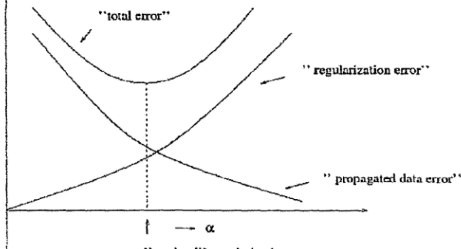
In any regularization method, the regularization parameter a plays a crucial role. As those of ordinary skill in the art will appreciate, the choice of the weight to give the terms con trolled by the regularization parameter represents a compro mise between accuracy and stability: if C is too large, the modeling error made by adding a penalty termin (12) leads to a poor approximation. If C is chosen too small, on the other hand, data errors may be immediately amplified too strongly. There are two general classes of options for choosing the parameter: A-priori rules define the regularization parameter as a function of the noise level only, i.e., C.C.(8), while in a-posteriori rules, C. depends both on the noise level and the
actual data, i.e., C. C.(8,y).
It should be kept in mind that error-free strategies, where
0 as C.->0, while the propagated data error grows without bound as C.->0. The optimal regularization parameter would be determined by the minimizer of the combined curve in FIG. 5, but is not computable from this curve, since the concrete computation of these curves would require knowing the exact solution of the inverse problem, in which case no further study would be required.
For Tikhonov regularization, a widely used a-posteriori
rule is the “discrepancy principle", where C.(Ö,y) is defined
as the solution of
If this equation (16) has no solution, which my happen for nonlinear problems, it can be replaced by a two-sided inequality. A quite complicated a posteriori strategy that always leads to optimal convergence rates can be found in 71. The papers quoted above concerning more general variational regularization methods also contains information on Suitable strategies for choosing parameters.
With respect to the numerical implementation of Tikhonov regularization (and more general variational regularization methods), one can relax the task of exactly solving problem (13) to looking for an element X. satisfying
for all x6D(F) with m a small positive parameter, see 24. Tikhonov regularization combined with finite dimensional approximation of X (and of F, see also Section 3.2) is dis cussed e.g., in 57, 58.
3.2. Iterative Methods
A first candidate for solving (9) in an iterative way could be Newton's method
starting from an initial guess X. Even if the iteration is well defined and F'() is invertible for every x6D(F), the inverse is usually unbounded for ill-posed problems (e.g., if F is con tinuous and compact the inverse of F" is also discontinuous). Hence, (18) is inappropriate in this form since each iteration requires one to solve a linear ill-posed problem, which would be unstable, and some regularization technique has to be used instead (see 23 for regularization methods for linear ill posed problems). For instance Tikhonov regularization applied to the linearization of (9) yields the Levenberg Mar quardt method (see 38)
where C is a sequence of positive numbers. Augmenting (19) by the term
(19)
25
30
35
40
45
50
55
60
65
first-order optimality condition for the nonlinear output least squares problem
1 (23)
sly - F(x)|| - min, x e D(F).
An alternative to Newton type methods like (19) and (21) are methods of steepest descent like the Landweber iteration
see 39, where the negative gradient of the functional in (23) determines the update direction for the current iterate. From
now on, we shall usex, in our notation of the iterates in order
to take into account possibly perturbed datay as defined in
(11).
In the ill-posed case, the iteration must not be arbitrarily continued because of the instability inherent in (9). Terminat ing the iteration properly is important to all iterative methods. An iterative method only can become a regularization method, if it is stopped “at the right time', i.e., only for a
suitable stopping index k does the iterate x, yield a stable
approximation to the solution x of (9). Due to the ill-posed
nature of the problem, a mere minimization of (23), i.e., an on-going iteration, leads to unstable results and to the typical error behavior shown in FIGS. 6 and 7. FIG. 6 is a plot of
|F(x)-y7 vs. k, while FIG. 7 is a plot of x-x vs. k.
While the error in the output decreases as the iteration number increases, the error in the parameter starts to increase after an initial decay. The stopping index plays the role of the regularization parameter.
Again, there are two classes of methods for choosing the regularization parameter, i.e., for the determination of the stopping index k, namely a-priori stopping rules with k=k.
(8) and a-posteriori rules with k=k.(Öy). Once more, the
discrepancy principle is a widely used representative for the latter a-posteriori rules, where k, now is determined by
(24)
for some sufficiently large td-0. As opposed to (16) for Tikhonov regularization, (25) now is a rule easy to imple ment, provided that an estimate for the data error as in (11) is available. The discrepancy principle for determining the
index k is based on stopping as soon as the residually'7-F
(x)|| is on the order of the data error, which is somehow the
best one should expect: All approximate solutions which give a residual not much larger than the data error are equally good
or bad if one has no other information, since the data are also
only know within this accuracy. For solving (9) when only
noisy data y with (11) are given, it would make no sense to
US 8,335,671 B2
23
regularization methods has been a hot topic in research recently, see, e.g., 31, 18, 49.
At first sight, Newton type methods might be thought to converge much faster than Landweber iteration; this is of course true in the sense that an approximation to a solution of (9) with a given accuracy can be obtained by fewer iteration steps. However, a single Newton type methods step (see (19) or (21)) is more expensive than a Landweber iteration (see (24)) and also the instability shows its effect earlier in Newton type methods and so that the iteration has to be stopped earlier. Thus, it cannot be said that Newton type methods are in general preferable for ill-posed problems to the much sim pler Landweber method. If especially efficient methods are used to solve the linear problems involved in each step of a Newton iteration, see 6, 12, Newton methods may be preferable but even that is not assured automatically.
Many iteration schemes for Solving inverse problems are formulated in terms of the Fréchet derivative and its adjoint operator. There are several notions of derivatives of nonlinear operators; all have in common that they are approximations of the nonlinear operator by linear operators in some “best possible' way; a convergence theory for direct and inverse problems for nonlinear equations usually requires conditions how this approximation is measured, the simplest and mostly used conditions summarized in the term Fréchet derivative. We show how, e.g., Landweber iteration is realized for the prototype parameter identification problem (10). The ideas presented then also apply in a similar way to other methods as (19) and (21). In a first step, we translate the problem into a Hilbert space framework and therefore consider the underly ing partial differential equation in its weak operator formula tion
For a set D(F) CX=H'(S2) (with s>d/2 whered is the dimen sion of S2) of admissible parameters q, the direct problem (26)
admits a unique solution A(q)'feHo"(S2) which will be
denoted by u?in order to emphasize its dependence on q. If we
regard for simplicity the case of distributed L-temperature
mea