DYNAMICS OF THE NONLINEAR RATIONAL DIFFERENCE EQUATION xn+1 =
Axn−αxn−β +Bxn−γ Cxn−αxn−β+Dxn−γ
Abdualrazaq Sanbo∗,∗∗∗, E. M. Elsayed∗,∗∗and Faris Alzahrani∗
∗Mathematics Department, Faculty of Science, King Abdulaziz University,
P. O. Box 80203, Jeddah 21589, Saudi Arabia
∗∗Department of Mathematics, Faculty of Science, Mansoura University,
Mansoura 35516, Egypt
∗∗∗General Studies Department, Jeddah College of Telecom and Electronics,
TVTC, B.P. 2816, Jeddah 21461, Saudi Arabia
e-mails: [email protected]; [email protected];
(Received 17 April 2018; accepted 12 June 2018)
In this article, we study the global stability and the asymptotic properties of the non-negative solutions of the non-linear difference equation:
xn+1 = Axn−αxn−β+Bxn−γ
Cxn−αxn−β+Dxn−γ, n= 0,1, ...,
whereα, β, γare positive integers,A, B, C, Dare positive real numbers and the initial conditions
x−p, x−p+1, ..., x−1, x0forp= max{α, β, γ}are arbitrary positive real numbers.
Key words : Difference equations; recursive sequences; local stability; global stability; boundedness; prime period two solution.
1. INTRODUCTION
The qualitative study of difference equations is a fertile research area and increasingly attracts many
mathematicians. This topic draws its importance from the fact that many real life phenomena are
modeled using difference equations. Examples from economy, biology, etc. can be found in [6, 9, 10,
It is known that nonlinear difference equations are capable of producing a complicated behavior
regardless its order. There has been a great interest in studying the global attractivity, the boundedness
character and the periodicity nature of nonlinear difference equations. For example, in the articles
[6, 9, 10, 25, 28] closely related global convergence results were obtained which can be applied to
nonlinear difference equations in proving that every solution of these equations conver to a period
two solution. The study of these equations is challenging and rewarding and is still in its infancy.
We believe that the nonlinear rational difference equations are of paramount importance in their own
right. Furthermore the results about such equations offer prototypes for the development of the basic
theory of the global behavior of nonlinear difference equations.
Elabbasy et al. [7, 8] investigated the global stability and the periodicity of the solutions of the
recursive sequence
xn+1= Axαxn+βxn−1+γxn−2 n+Bxn−1+Cxn−2 and
xn+1= Axαxn−l+βxn−k n−l+Bxn−k
Zayed [38] studied the global stability and the asymptotic properties of the nonnegative solutions
of the nonlinear difference equation
xn+1 =Axn+Bxn−k+ pxn+xn−k q+xn−k
Our aim in this paper is to investigate the behavior of the solution of the following nonlinear
difference equation
xn+1= CxAxn−αxn−β+Bxn−γ n−αxn−β+Dxn−γ
, n= 0,1, ..., (1)
whereA, B, C, D are positive real numbers, α, β, γ are positive integers and the initial conditions
x−p, x−p+1, ..., x−1, x0forp= max{α, β, γ}are arbitrary positive real numbers.
Here, we recall some notations and results which will be useful in our investigation. LetI be
some interval of real numbers and let
f :Ik+1→I,
be a continuously differentiable function. Then for every set of initial conditionsx−k, x−k+1, x−k+2, ...,
x0 ∈I, the difference equation
xn+1=f(xn, xn−1, ..., xn−k), n= 0,1, ..., (2)
has a unique solution{xn}∞n=−k.
Definition 1 — The difference equation (2) is said to be persistence if there exist numbersmand
exists a positive integerN, which depends on the initial conditions, such that
m≤xn≤M for all n≥N.
Definition 2 — (Equilibrium Point). A pointx¯ ∈ I is called an equilibrium point of Eq. (2) if
¯
x =f(¯x,x, ...,¯ x¯). That is,xn = ¯xforn≥ 0, is a solution of Eq. (2), or equivalently,x¯is a fixed
point off.
Definition 3 — (Stability).
• The equilibrium pointx¯of Eq. (2) is locally stable if for everyε >0, there existsδ >0such
that for allx−k, x−k+1, x−k+2, ..., x0 ∈I,with
|x−k−x¯|+|x−k+1−x¯|+|x−k+2−x¯|+...+|x0−x¯|< δ,
we have|xn−x¯|< ε, for alln≥ −k.
• The equilibrium pointx¯of Eq. (2) is locally asymptotically stable ifx¯is locally stable solution
of Eq. (2) and there existsγ >0, such that for allx−k, x−k+1, x−k+2, ..., x0∈I,with
|x−k−x¯|+|x−k+1−x¯|+|x−k+2−x¯|+...+|x0−x¯|< δ,
we have lim
n→∞xn= ¯x.
• The equilibrium pointx¯of Eq. (2) is global attractor if for allx−k, x−k+1, ..., x0 ∈I we have
lim
n→∞xn= ¯x.
• The equilibrium pointx¯of Eq. (2) is globally asymptotically stable ifx¯is locally stable, andx¯
is also a global attractor of Eq. (2).
• The equilibrium pointx¯of Eq. (2) is unstable ifx¯is not locally stable.
The linearized equation of Eq. (2) about the equilibriumx¯is the linear difference equation
yn+1= k X
i=0
∂f(¯x,x, ...,¯ x¯) ∂xn−i yn−i
Theorem 1 — Assume that p, q ∈ Randk ∈ {0,1,2, ...}. Then |p|+|q| < 1 is a sufficient
condition for the asymptotic stability of the difference equation
Remark 1 : The theorem can be easily extended to a general linear equations of the form
xn+k+p1xn+k−1+...+pkxn= 0, n= 0,1, ..., (3)
wherep1, p2, ..., pk ∈ Randk ∈ {0,1,2, ...}. Then Eq. (3) is asymptotically stable provided that k
X
i=0
|pi|<1.
Theorem 2 — Letf ∈ C[Ik+1, I]for some intervalI of the real numbers and for some
non-negative integerk, and consider the difference equation (2). Let{xn}∞n=−k be a solution of Eq.(2),
and suppose that there exist constantsh∈IandH∈Isuch that
h≤xn≤H for all n≥ −k.
Letl0be a limit point of the sequence{xn}∞n=−k. Then the following statements are true.
(i) There exists a solution{Ln}∞n=−∞of Eq. (2), called a full limiting sequence of{xn}∞n=−k, such
thatL0 =l0, and such that for everyN ∈ {...,−1,0,1, ...},LN is a limit point of{xn}∞n=−k.
(ii) For everyi0 ≤ −k, there exists a subsequence{xri}∞i=0of{xn}∞n=−ksuch that
LN = limn→∞xri+N for every N ≥ −i0.
2. LOCALSTABILITY OFEQ. (1)
In this section we investigate the local stability character of the solutions of Eq. (1). If Eq. (1) admits
an equilibrium pointx¯thenx >¯ 0and
¯
x= Ax¯2+Bx¯ Cx¯2+Dx¯ =
Ax¯+B Cx¯+D,
or
¯
x(Cx¯+D) =Ax¯+B,
or also
Cx¯2+ (D−A)¯x−B = 0,
Let∆ = (D−A)2+ 4BC. Then Eq. (1) admits a unique positive equilibrium point given by
¯
x= A−D+
p
(D−A)2+ 4BC
Define the following function
f : (0,∞)3 →(0,∞)
f(u, v, w) = Auv+Bw Cuv+Dw.
(5)
Therefore it follows that
fu(u, v, w) =
(AD−BC)vw
(Cuv+Dw)2 , fv(u, v, w) =
(AD−BC)uw
(Cuv+Dw)2 , fw(u, v, w) =−
(AD−BC)uv (Cuv+Dw)2 .
Then
fu(¯x,x,¯ x¯) =(AD−BC)
(Cx¯+D)2 , fv(¯x,x,¯ x¯) =
(AD−BC)
(Cx¯+D)2 , fw(¯x,x,¯ x¯) =−
(AD−BC) (Cx¯+D)2 .
Leta= (AD−BC)
(Cx¯+D)2 then the linearized equation of Eq. (1) aboutx¯is
yn+1−ayn−α−ayn−β+ayn−γ = 0. (6)
whose characteristic equation is given by
λγ+1−aλγ−α−aλγ−β+a= 0.
Theorem 3 — Assume that
|AD−BC|< (Cx¯+D)2 3 . Then the equilibrium point of Eq. (1) is locally asymptotically stable.
PROOF: It follows from Theorem 1 that Eq. (6) is asymptotically stable if
|a|+|a|+|a|=
¯ ¯ ¯
¯((ADCx¯−+BCD)2) ¯ ¯ ¯ ¯+
¯ ¯ ¯
¯((ADCx¯−+BCD)2) ¯ ¯ ¯ ¯+
¯ ¯ ¯
¯((ADCx¯−+BCD)2) ¯ ¯ ¯
¯= 3|(ADCx¯−+BCD)2| <1,
and so,
|AD−BC|< (Cx¯+D)2 3 .
The proof is complete.
3. GLOBAL ATTRACTOR OF THEEQUILIBRIUMPOINT OFEQ. (1)
In this section we investigate the global attractivity character of solutions of Eq. (1).
PROOF: Let {xn}∞n=−p be a solution of Eq. (1) and again letf be the function defined by Eq.
(5), then we can easily see that the functionf(u, v, w)is increasing inu, vand decreasing inw. Thus
from Eq. (1), we see that
xn+1 = CxAxn−αxn−β+Bxn−γ n−αxn−β+Dxn−γ
≤ Axn−αxn−β+B×0
Cxn−αxn−β+D×0 = A C.
Then
xn≤ A
C =H for all n≥1.
xn+1 = Axn−αxn−β+Bxn−γ Cxn−αxn−β+Dxn−γ
≥ A×0 +Bxn−γ
C×0 +Dxn−γ
= B D.
Then
xn≥ BD =h for all n≥1.
We see therefore that
h= B
D ≤xn≤ A
C =H for all n≥1.
It follows by the method of Full Limiting sequences that there exist solutions{In}∞n=−∞and{Sn}∞n=−∞
of Eq.(1) with
I =I0 = limn→∞infxn≤n→∞lim supxn=S0 =S,
where
In, Sn∈[I, S], n= 0,−1, ...
It suffices to show thatI =S.
Now it follows from Eq.(1) that
I = AIn−α−1In−β−1+BIn−γ−1 CIn−α−1In−β−1+DIn−γ−1 ≤
AS2+BI
CS2+DI,
and so
AS2+BI−DI2 ≥CS2I → AS2I+BI2−DI3≥CS2I2.
Similarly, it follows from Eq.(1) that
S = ASn−α−1Sn−β−1+BSn−γ−1 CSn−α−1Sn−β−1+DSn−γ−1 ≥
AI2+BS CI2+DS,
and so
It follows that
AI2S+BS2−DS3 ≤CI2S2≤AS2I+BI2−DI3.
or also
AS2I+BI2−DI3−AI2S−BS2+DS3= (S−I)£(A−D)SI−(BS+BI+DS2+DI2)¤≥0.
Hence
I ≥S if (A−D)SI−(BS+BI+DS2+DI2)<0.
Now, we know thatD ≥Aand so it follows thatI ≥S. ThereforeI =S. This completes the
proof.
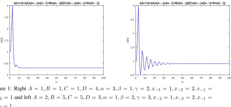
For confirming the local and global stability results, we consider two numerical examples. For
A = 1, B = 1, C = 1, D = 4, α = 3, β = 1, γ = 2, x−3 = 1, x−2 = 2, x−1 = 3, x0 = 1which
satisfy the stability conditions then Eq.(1) admits an equilibrium pointx¯= 0.30278which is a global
attractor of Eq.(1) (See Figure 1, left). ForA = 2, B = 5, C = 5, D = 3, α = 1, β = 2, γ = 3, x−3 = 1, x−2 = 2, x−1 = 3, x0 = 1which satisfy also the stability conditions then Eq.(1) admits
an equilibrium pointx¯= 0.9050which is a global attractor of Eq.(1) (See Figure 1, right).
n
0 10 20 30 40 50 60 70 80 90 100
x(n)
0 0.5 1 1.5 2 2.5
3 x(n+1)=(Ax(n-α)x(n-β)+Bx(n-γ))/(Cx(n-α)x(n-β)+Dx(n-γ))
n
0 10 20 30 40 50 60 70 80 90 100
x(n)
0.5 1 1.5 2 2.5
[image:7.612.91.551.434.648.2]3 x(n+1)=(Ax(n-α)x(n-β)+Bx(n-γ))/(Cx(n-α)x(n-β)+Dx(n-γ))
Figure 1: RightA = 1, B = 1, C = 1, D = 4, α = 3, β = 1, γ = 2, x−3 = 1, x−2 = 2, x−1 =
3, x0 = 1and leftA = 2, B = 5, C = 5, D = 3, α= 1, β = 2, γ = 3, x−3 = 1, x−2 = 2, x−1 =
3, x0= 1.
4. BOUNDEDNESS OFSOLUTIONS OFEQ. (1)
Theorem 5 — Every solution of Eq. (1) is bounded and persists.
PROOF: Let{xn}∞n=−pbe a solution of Eq. (1). It follows from Eq. (1) that
xn+1 = Axn−αxn−β+Bxn−γ Cxn−αxn−β+Dxn−γ
= Axn−αxn−β
Cxn−αxn−β+Dxn−γ +
Bxn−γ
Cxn−αxn−β+Dxn−γ
≤ Axn−αxn−β
Cxn−αxn−β
+Bxn−γ Dxn−γ =
µ
A
C +
B D
=M
Hence
xn≤ µ
A C +
B D
=M for all n≥1. (7)
Now we wish to show that there existsm >0such that
xn≥m for all n≥1.
The change of variables,yn= x1
n, gives Eq. (1) in the form
1 yn+1 =
A yn−αyn−β
+ B yn−γ
C yn−αyn−β
+ D yn−γ
= Ayn−γ+Byn−αyn−β Cyn−γ+Dyn−αyn−β,
or in the equivalent form
yn+1 =
Cyn−γ+Dyn−αyn−β Ayn−γ+Byn−αyn−β
= Cyn−γ Ayn−γ+Byn−αyn−β
+ Dyn−αyn−β Ayn−γ+Byn−αyn−β
≤ Cyn−γ
Ayn−γ
+Dyn−αyn−β Byn−αyn−β
=
µ
C A +
D B
Thus we obtain
xn= y1 n ≥
1
µ
C A +
D B
¶ = AB
BC+AD =m for all n≥1. (8)
One deduces from (7) and (8) that
Therefore every solution of Eq.(1) is bounded and persists.
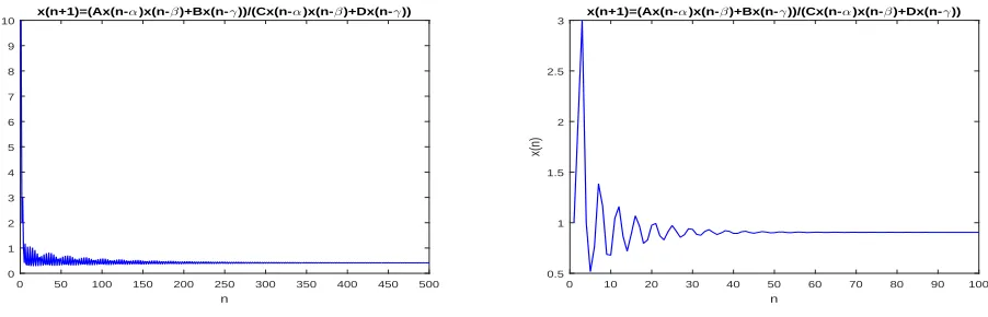
For confirming the boundedness results, we consider the following two numerical examples. For
A = 2, B = 1, C = 1, D = 4, α = 2, β = 2, γ = 3, x−3 = 10, x−2 = 2, x−1 = 3, x0 = 4and
A = 2, B = 5, C = 5, D = 3, α = 1, β = 2, γ = 3, x−3 = 1, x−2 = 2, x−1 = 3, x0 = 1. The
solution is bounded and persists (See Figure 2).
n
0 50 100 150 200 250 300 350 400 450 500
x(n)
0 1 2 3 4 5 6 7 8 9
10 x(n+1)=(Ax(n-α)x(n-β)+Bx(n-γ))/(Cx(n-α)x(n-β)+Dx(n-γ))
n
0 10 20 30 40 50 60 70 80 90 100
x(n)
0.5 1 1.5 2 2.5
[image:9.612.101.552.240.385.2]3 x(n+1)=(Ax(n-α)x(n-β)+Bx(n-γ))/(Cx(n-α)x(n-β)+Dx(n-γ))
Figure 2: RightA = 2, B = 1, C = 1, D = 4, α = 2, β = 2, γ = 3, x−3 = 10, x−2 = 2, x−1 =
3, x0 = 4and leftA = 2, B = 5, C = 5, D = 3, α= 1, β = 2, γ = 3, x−3 = 1, x−2 = 2, x−1 =
3, x0= 1.
5. PERIODICITY OFSOLUTIONS OFEQ. (1)
In this section we study the existence of prime period two solutions of Eq. (1).
Theorem 6 — ForA=D, Eq. (1) has prime period two solutions if and only ifBC >4A2,γ is
odd,αandβare even.
PROOF: First suppose that there exists a prime period two solutions
..., p, q, p, q, ...
of Eq.(1). We see from Eq.(1) that
p= Aq2+Bp Cq2+Dp
and
Hence
Cq2p+Dp2 =Aq2+Bp (9)
and
Cqp2+Dq2 =Ap2+Bq. (10)
Subtracting Eq.(10) from Eq.(9) gives
Cqp(q−p) +D(p2−q2) =A(q2−p2) +B(p−q).
Sincep6=q, it follows that
Cqp+D(p+q) =A(q+p) +B. (11)
Again adding Eq.(9) and Eq.(10) yields
Cqp(q+p) +D(p2+q2) =A(q2+p2) +B(p+q).
Asp+q 6= 0then
Cqp+D(p
2+q2)
p+q =A
(p2+q2)
p+q +B. (12)
Subtracting Eq.(12) from Eq.(11) gives
D
µ
(p2+q2)
p+q −(p+q)
=A
µ
(p2+q2)
p+q −(p+q)
.
Since (p
2+q2)
p+q 6= (p+q)thenA=D. From Eq.(11), we deduce that
qp= B C.
From Eq.(9), we deduce that
Bq+Dp2 =Aq2+Bp (13)
and from Eq. (10), we deduce that
Bp+Dq2=Ap2+Bq. (14)
Subtracting Eq.(14) from Eq.(13) we obtain
2A(p2−q2) + 2B(q−p) = 0.
Sincep6=q, then
Thenpandqare positive solutions of equation
t2− B
At+ B
C = 0. (15)
This means that
∆ = B2 A2 −4
B C >0
and then
B A2 >
4
C → BC >4A
2
Conversely suppose that condition (i) is true. We will show that Eq.(1) has a prime period two
solution. Assume that
p= B A −
r
B2
A2 −4
B C 2 = B 2A ³ 1− r
1−4A
2 BC ´ and q= B A + r B2 A2 −4
B C 2 = B 2A ³ 1 + r
1− 4A2
BC
´
We see from condition (i) that1− 4A
2
BC >0, thereforepandqare distinct positive real numbers.
Set
x−α =q, x−γ =p, x−β =q, ..., and x0 =p.
We wish to show that
x1=x−1=q and x2 =x0=p.
It follows from Eq.(1) that
x1 = CxAx−αx−β+Bx−γ −αx−β+Dx−γ =
Ap2+Bq
Cp2+Aq =
A Ã B 2A ³ 1− r
1− 4A2
BC
´!2
+B B 2A
³
1 +
r
1−4A2
BC ´ C Ã B 2A ³ 1− r
1−4A2
BC
´!2
+AB 2A
³
1 +
r
1−4A2
BC ´ = B A Ã 1− r
1− 4A
2 BC !2 + 2 ³ 1 + r
1−4A
2 BC ´ BC A2 Ã 1− r
1−4A2
BC !2 + 2 ³ 1 + r
1−4A2
BC
= B A
4−4A2
BC BC
A2 Ã
2−4A2
BC −2
r
1−4A2
BC ! + 2 ³ 1 + r
1− 4A2
BC ´ = 4( B A − A C) 2BC
A2 −4−
2BC A2
r
1−4A2
BC + 2 + 2
r
1−4A2
BC = 4(B A − A C) µ 2BC A2 −2
¶ Ã
1−
r
1−4A
2
BC
!
Multiplying the denominator and numerator by
Ã
1 +
r
1−4A2
BC
!
= 2Aq
B gives
x1=
4(B A − A C) Ã 1 + r
1−4A
2
BC
!
µ
2BC A2 −2
4A2
BC = 4(B A − A C) 2Aq B µ 2BC A2 −2
4A2
BC =
µ
1− A
2
BC
µ
1− A2
BC
¶q=q.
Similarly as before one can easly show that
x2 =p.
Then it follows by induction that
x2n=p and x2n+1 =q for all n≥ −1.
Thus Eq.(1) has the positive prime period two solution
..., p, q, p, q, ...
wherepandqare the distinct roots of the quadratic equation (15) and the proof is complete.
For confirming the periodicity results, we consider the following two numerical examples. For
A = 6, B = 30, C = 5, D = 6, α = 4, β = 2, γ = 1, x−4 = 2, x−3 = 3, x−2 = 2, x−1 =
3, x0 = 2which satisfy the periodicity conditions then Eq.(1) has positive prime period two solutions
n
0 10 20 30 40 50 60 70 80 90 100
x(n)
2 2.1 2.2 2.3 2.4 2.5 2.6 2.7 2.8 2.9
3 x(n+1)=(Ax(n-α)x(n-β)+Bx(n-γ))/(Cx(n-α)x(n-β)+Dx(n-γ))
n
0 10 20 30 40 50 60 70 80 90 100
x(n)
2 2.5 3 3.5 4 4.5
5 x(n+1)=(Ax(n-α)x(n-β)+Bx(n-γ))/(Cx(n-α)x(n-β)+Dx(n-γ))
Figure 3: RightA = 6, B = 30, C = 5, D = 6, α = 4, β = 2, γ = 1, x−4 = 2, x−3 = 3, x−2 =
2, x−1 = 3, x0 = 2and leftA= 10, B= 70, C = 7, D= 10, α= 4, β= 4, γ= 5, x−5= 5, x−4 =
2, x−3 = 5, x−2 = 2, x−1= 5, x0 = 2.
Since A = 10, B = 70, C = 7, D = 10, α = 4, β = 4, γ = 5, x−5 = 5, x−4 = 2, x−3 =
5, x−2 = 2, x−2 = 5, x0 = 2which satisfy the periodicity conditions then Eq.(1) has positive prime
period two solutions...,5,2,5,2, ...(See Figure 3, left).
Lemma 1 —
(i) Ifα,β andγ are odd, then Eq. (1) has no positive solutions of prime period two.
(ii) Ifα,β andγ are even, then Eq. (1) has no positive solutions of prime period two.
(iii) Ifα,γ are odd andβis even (respectively ifβ,γ are odd andαis even), then Eq. (1) has no
positive solutions of prime period two.
(iv) Ifαis odd,β andγ are even (respectively ifα,γ are even andβ is odd), then Eq. (1) has no
positive solutions of prime period two.
PROOF: Suppose that there exists a prime period two solutions
..., p, q, p, q, ...
of Eq.(1).
We prove this for the first two cases whereγ,αandβare odd and for the case whereα,β andγ
(i) Assume thatα,βandγare odd. We see from Eq.(1) that
p= Ap2+Bp Cp2+Dp =
Ap+B Cp+D,
and
q= Aq2+Bq Cq2+Dq =
Aq+B Cq+D.
Hence
Cp2+ (D−A)p−B = 0,
and
Cq2+ (D−A)q−B = 0.
Thenpandqare positive solutions of equation
Ct2+ (D−A)t−B = 0.
SinceB >0, then one of the solutions is negative. This is a contradiction. Thus Eq.(1) has no
prime period two solution.
(ii) Assume thatα,βandγare even. We see from Eq.(1) that
q = Ap2+Bp Cp2+Dp =
Ap+B Cp+D,
and
p= Aq2+Bq Cq2+Dq =
Aq+B Cq+D.
Hence
Cpq+Dq=Ap+B, (16)
and
Cpq+Dp=Aq+B. (17)
Subtracting Eq.(17) from Eq.(16) we obtain
(D+A)(q−p) = 0.
SinceD+A6= 0, then
p=q
6. CONCLUSION
This paper discussed local and global stability, boundedness and periodicity of the solutions of
Eq.(1). In Section 2 we proved that Eq.(1) admits a unique positive equilibrium point given by
¯
x = D−A+
p
(D−A)2+ 4BC
2C and that if|AD−BC| <
(Cx¯+D)2
3 then this equilibrium
point is locally asymptotically stable. In Section 3 we showed that the unique equilibrium of Eq.(1) is
globally asymptotically stable ifD≥A. In Section 4 we proved that the solution of Eq.(1) is always
bounded and persists. In Section 5 we gave some conditions on the periodicity of solutions of Eq.(1).
ACKNOWLEDGEMENT
This article was funded by the Deanship of Scientific Research (DSR), King Abdulaziz University,
Jeddah. The authors, therefore, acknowledge with thanks DSR technical and financial support.
REFERENCES
1. M. Abu Alhalawa and M. Salah, Dynamics of higher order rational difference equation, J. Nonlinear Anal. Appl., 8(2) (2017), 363-379.
2. N. Battaloglu, C. Cinar, and I. Yalc¸inkaya, The dynamics of the difference equation, Ars Combinatoria, 97 (2010), 281-288.
3. F. Belhannache, N. Touafek, and R. Abo-Zeid, On a higher-order rational difference equation, J. Appl. Math.&Informatics, 34(5-6) (2016), 369-382.
4. F. Bozkurt, I. Ozturk, and S. Ozen, The global behavior of the difference equation, Stud. Univ. Babes¸-Bolyai Math., 54(2) (2009), 3-12.
5. E. M. Elabbasy and E. M. Elsayed, Dynamics of a rational difference equation, Chinese Annals of Mathematics, Series B, 30 (2009), 187-198.
6. E. M. Elabbasy, H. El-Metwally, and E. M. Elsayed, On the difference equationsxn+1= αxn−k β+γQki=0xn−i
,
J. Conc. Appl. Math., 5(2) (2007), 101-113.
7. E. M. Elabbasy, H. El-Metwally, and E. M. Elsayed, Global attractivity and periodic character of a fractional difference equation of order three, Yokohama Mathematical, 53 (2007), 89-100.
8. E. M. Elabbasy, H. El-Metwally, and E. M. Elsayed, On the difference equationxn+1= αxn−l+βxn−k Axn−l+Bxn−k
, Acta Mathematica Vietnamica, 33(1) (2008), 85-94.
9. E. M. Elabbasy, H. El-Metwally, and E. M. Elsayed, On the difference equation xn+1 = axn −
bxn
cxn−dxn−1
10. M. M. El-Dessoky, On the difference equationxn+1 = axn−1+bxn−k+ cxn−s
dxn−s−e
, Math. Meth. Appl. Sci., 40 (2017), 535-545.
11. H. El-Metwally and E. M. Elsayed, Form of solutions and periodicity for systems of difference equa-tions, Journal of Computational Analysis and Applicaequa-tions, 15(5) (2013), 852-857.
12. E. M. Elsayed, Behavior and expression of the solutions of some rational difference equations, Journal of computational analysis and applications, 15(1) (2013), 73-81.
13. E. M. Elsayed, Qualitative properties for a fourth order rational difference equation, Acta Applicandae Mathematicae, 110(2) (2010), 589-604.
14. E. M. Elsayed, On the global attractivity and the solution of recursive sequence, Studia Scientiarum Mathematicarum Hungarica, 47(3) (2010), 401-418.
15. E. M. Elsayed, Qualitative behavior of difference equation of order three, Acta Scientiarum Mathemati-carum (Szeged), 75(1-2) (2009), 113-129.
16. E. M. Elsayed, Dynamics of a rational recursive sequence, Inter. J. Differ. Equations, 4(2)(2009), 185-200.
17. E. M. Elsayed, Qualitative behavior ofsrational recursive sequence, Indagationes Mathematicae, New Series, 19(2) (2008), 189-201.
18. E. M. Elsayed, F. Alzahrani, and H. S. Alayachi, Formulas and properties of some class of nonlinear difference equations, Journal of Computational Analysis and Applications, 24(8) (2018), 1517-1531.
19. E. M. Elsayed and A. Khaliq, The dynamics and global attractivity of a rational difference equation, Advanced Studies in Contemporary Mathematics, 26(1) (2016), 183-202.
20. E. M. Elsayed and T. F. Ibrahim, Periodicity and solutions for some systems of nonlinear rational differ-ence equations, Hacettepe Journal of Mathematics and Statistics, 44(6) (2015), 1361-1390.
21. E. M. Elsayed and T. F. Ibrahim, Solutions and periodicity of a rational recursive sequences of order five, Bulletin of the Malaysian Mathematical Sciences Society, 38(1) (2015), 95-112.
22. E. M. Elsayed and A. M. Ahmed, Dynamics of a three-dimensional systems of rational difference equa-tions, Mathematical Methods in The Applied Sciences, 39(5) (2016), 1026-1038.
23. T. F. Ibrahim, Closed form expressions of some systems of nonlinear partial difference equations, Jour-nal of ComputatioJour-nal AJour-nalysis and Applications, 23(3) (2017), 433-445.
24. V. L. Kocic and G. Ladas, Global behavior of nonlinear difference equations of higher order with appli-cations, Kluwer Academic Publishers, Dordrecht, 1993.
26. K. Liu, P. Li, F. Han, and W. Zhong, Global dynamics of nonlinear difference equation xn+1 = xn
xn−1xn−2
, Journal of Computational Analysis and Applications, 24(6) (2018), 1125-1132.
27. O. Ocalan, H. Ogunmez, and M. Gumus, Global behavior test for a non-linear difference equation with a period-two coefficient, Dynamics of Continuous, Discrete and Impulsive Systems Series A: Mathemat-ical Analysis, 21 (2014), 307-316.
28. M. Saleh and S. Abu-Baha, Dynamics of a higher order rational difference equation, Appl. Math. Comp., 181(1) (2006), 84-102.
29. D. Simsek and F. Abdullayev, On the recursive sequencexn+1=
xn−(4k+3) 1 +Q2t=1xn−(k+1)t−k
, J. Math. Sci.,
6(222) (2017), 762-771.
30. T. Sun, Y. Zhou, G. Su, and Bin Qin, Eventual periodicity of a max-type difference equation system, Journal of Computational Analysis and Applications, 24(5) (2018), 976-983.
31. C. Y. Wang, X. J. Fang, and R. Li, On the solution for a system of two rational difference equations, Journal of Computational Analysis and Applications, 20(1) (2016), 175-186.
32. C. Y. Wang, X. J. Fang, and R. Li, On the dynamics of a certain four-order fractional difference equa-tions, Journal of Computational Analysis and Applicaequa-tions, 22(5) (2017), 968-976.
33. C. Wang, Y. Zhou, S. Pan, and R. Li, On a system of three max-type nonlinear difference equations, Journal of Computational Analysis and Applications, 25(8) (2018), 1463-1479.
34. Y. Yazlik, E. M. Elsayed, and N. Taskara, On the behaviour of the solutions of difference equation systems, Journal of Computational Analysis and Applications, 16(5) (2014), 932-941.
35. T. Yi and Z. Zhou, Periodic solutions of difference equations, J. Math. Anal. Appl., 286 (2003), 220-229.
36. E. M. E. Zayed and M. A. El-Moneam, On the qualitative study of the nonlinear difference equation
xn+1= αxn−σ
β+γxpn−τ, Fasciculi Mathematici, 50 (2013), 137-147.
37. E. M. E. Zayed and M. A. El-Moneam, On the global attractivity of two nonlinear difference equations, J. Math. Sci., 177 (2011), 487.
38. E. M. E. Zayed, Dynamics of the nonlinear rational difference equation xn+1 = Axn +Bxn−k +
pxn+xn−k
q+xn−k