Investigating the Temporary and Permanent
Influential Variables on Iran Inflation Using
TVP-DMA Models
Mohsen Khezri*1, Seyed Ehsan Hosseinidoust2,
Mohammad Kazem Naziri3
Received: 2017, October 30 Accepted: 2017, December 19
Abstract
nflation forecast is one of the tools in targeting inflation by the central bank. The most important problem of previous models to forecast the inflation is that they could not provide a correct prediction over time. However, the central bank policymakers shall seek to create economic stability by ignoring the short-term and temporary changes in price and regarding steady inflation. On this basis, in the present paper, it has been aimed to provide nonlinear dynamic models to simulate the inflation in the economy of Iran using quarterly data referring to 1988- 2012 as well as TVP-DMA and TVP-DMS models. These models can provide changes in input variables as well as changes in the coefficients of the model over time. Based on the results, the possibility of growth of currency in circulation, economic growth, also the growth of deposits either visual or non-visual variables, is more remarkable in modeling of inflation in economy of Iran. In addition, the predictive power of dynamic models presented in this study is more than other models.
Keywords: Dynamic Modeling, Inflation Forecasting, TVP-DMS Model.
JEL Classification: E31, E37, C11, C53.
1. Introduction
Preliminary studies in inflation forecast was mostly in the form of traditional Phillips curve that showed the relationship between
1. Department of Economics, Faculty of Economics and Social Science, Bu-Ali Sina University, Hamedan, Iran (Corresponding Author: [email protected]).
2. Department of Economics, Faculty of Economics and Social Science, Bu-Ali Sina University, Hamedan, Iran ([email protected]).
3. Department of Economics, Faculty of Economics and Social Science, Bu-Ali Sina University, Hamedan, Iran ([email protected]).
inflation and unemployment; but, after a few decades and especially after Lucas critique, original Phillips curve was being affected greatly (King, 2008). In 1970s, stagflation happened in the economy by the incidence of crises and shocks. According to the teachings from Phillips curve, policymakers preferred the rise in inflation than in unemployment. But, as Friedman and Philips had predicted, the unemployment rate returned to the natural rate, and this time with a higher rate of inflation. Thus, the initial structural interpretation of the Phillips curve has lost its credibility. With the expiration of a period of low inflation in 1980s and early 1990s, economists studied the structural interpretation of the Phillips curve once again. From mid-1990s, assuming the neutrality of money, economists began to enter the rigidity of nominal prices into general equilibrium models. Therefore, the new curves related the actual and expected inflation not only to the unemployment rate, but the scale of the final total cost. Since the final cost in the original Phillips new Keynesian curve model stimulate the inflation, it makes the matching of data difficult; thus, Phillips new Keynesian curve model was moderated by inputting intervals in inflation (Stock and Watson, 2008).
time, and sometimes it was observed that some models could predict the estimation of recession well, and some others could predict the estimation of the boom better. Such assumption in the use of experimental results causes limitations for policymakers of the central bank, because the central bank policymakers should not react to temporary changes in the price level, and should ignore the short-term and transient changes in prices and by considering a steady inflation seek to create economic stability. in recent years, major studies conducted in the field of inflation forecast have often been in the form of time varying parameters (TVP) models, Monte Carlo Markov Chain (MCMC) (Nakajima, 2011). Such an assumption is also considered in this study, in the way that using a dynamic model averaging DMA proposed by Raftery et al. (2007) in combination with TVP model, and applying the method of Stock and Watson (1999 and 2008), the power of approved variables has been investigated through the theoretical foundations of the Phillips curve and the main variables in the domestic empirical studies that had significant impact on inflation, and non-linear impact on inflation in Iran. This paper is organized in four parts, in the second part, literature review is presented; in the third part theoretical basis of dynamic models are indicated, and the fourth part provides analysis of the results.
2. Literature Review
countries of the mentioned rule, the theoretical critique of the Phillips curve could not decline its position. Even issues raised by Philips (1967) and Friedman (1968) in which the volatility of existing indices have been underlined in the Phillips curve, they could not reduce the importance of the Phillips curve as long as the experimental findings have not been confirmed; however, Lucas critique (1976), which is considered an experimental criticism, has faded a considerable influence and importance of a clear rule stated by the Phillips curve. Lucas insists that the structure of a macroeconomic model consists of optimal decision rules with economic agents (people), but these optimal decisions are systematically changing in the process of decision making by policymakers. As a result, any change in policy will systematically alter the structure of macroeconomic models (Lucas, 1976). Lucas’s hypothesis became a tool for economic policymakers to not to rely on the Phillips curve to predict the effects of the economic policies in future. After proposing Lucas critique, several studies using different econometric methods investigated it, and most of these studies have confirmed the lack of stability of indices. The achievement of such results may expose the application of the Phillips curve in economic analysis and its usage as a tool for policymakers to a problem. Due to the fact that in developing countries like Iran that are most vulnerable to structural changes in their economy, paying attention to these issues will be more remarkable. Estrella and Fuhrer (2003) argued that Lucas critique itself was not a theoretical result, but a warning that reveals the importance of applying parameters stability tests in macroeconomic models; therefore, econometric techniques to check the stability of parameters are essential for testing Lucas critique. These obstacles led to the original Phillips curve experiencing a lot of changes.
money supply and economic activity volume were also present. In the paper, Stock and Watson used the dynamic method of unobserved components stochastic volatility. The results of the study showed a close relationship between the volumes of recent economic activity with inflation in the future. In 2005, Primiceri used time varying parameters with structural vector autoregressive approach TVP-VAR that was the outcome of a doctoral thesis written at Princeton University, United States, and sought inflation forecast for the United States. In this study, researchers, using this model, showed that at any one time which variables could predict inflation, and in addition it could determine the trend of inflation. The main affecting factors were liquidity, unemployment, and interest rates, among which the greatest impact related to liquidity, interest rates, and unemployment, respectively. Groen et al. (2009) predicted the inflation in America's economy in the Federal Reserve New York. This study, which was published in the November 2010 report of America Federal Reserve, carried out the structural failure rate of inflation forecast with the help of Bayesian model. This study was based on empirical data conducted during 1960-2008 in the United States. Variables upon which the inflation was predicted were real GDP, liquidity, uncertainty of inflation intervals. Researchers made predictions using MCMC algorithms; moreover, Monte Carlo models as well as TVP-AR, SB-AR, and UC-SV models were also estimated. In the study, the relationship between each of the macroeconomic variables such as oil prices, real GDP, investment with inflation was determined; In addition inflation persistence probability was calculated at any period of time.
TVP-AR, TVP-VTVP-AR, TVP-SVTVP-AR, and compared their predictive power. The other result of the study was sensitivity analysis of inflation reaction to changes in macroeconomic.
3. Theoretical Basis 3.1 Dynamic Models
Before investigating the above models, it is required to present the main features of these models and their role in improving the estimated results of economic modeling:
1.Given that the computational method in above models is based on Kalman filter, the estimated coefficients vary over time. In terms of structural breaks and cycle changes in time series (which is the main feature of time series in Iran’s economy), the conventional methods are not enough to calculate the parameters, in this condition Kalman filter provides the possibility of modeling of the above facts with variable coefficients over time, (Stock and Watson, 2008).
2.In this type of models, the number of variables and estimators can be high. Gruen et al. used 10 estimators in their study, so that even in Factor models (Stock and Watson, 1999) the number of variables can also be more than that. Increasing number of variables creates large and bulky models. When there are 𝑚 estimators in the models, selection of model’s estimator may be the main challenge for modeling, and researcher can estimates 2𝑚 different models (according to the number of different
subsets of 𝑚 variables). In these circumstances, in most studies, researchers use TVP Bayesian models to estimate the model (like the study by Avramov, 2002; Cremers, 2002; Koop and Potter, 2004).
In the present study, dynamic model averaging DMA proposed by Raftery et al. (2007) has been used. Raftery et al. (2007) suggested dynamic model selection DMS along with DMA that will be discussed further. Standard models of State-Space methods and in particular Kalman filter is as follows:
𝜃𝑡 = 𝜃𝑡−1+ 𝜇𝑡 (2)
where 𝑦𝑡is inflation, 𝑧𝑡 = [1, 𝑥𝑡−1, 𝑦𝑡−1, ⋯ , 𝑦𝑡−𝑝] is a 1 × 𝑚 vector of the intercept estimators and variable interruption depending on model, and 𝜃𝑡 = [𝜑𝑡−1, 𝛽𝑡−1, 𝛾𝑡−1, ⋯ , 𝛾𝑡−𝑝]is an 𝑚 × 1 vector of coefficients (states), 𝜀𝑡~𝑁(0, 𝐻𝑡) and 𝜇𝑡~𝑁(0, 𝑄𝑡) that have a normal distribution with zero mean and variance of 𝐻𝑡 and 𝑄𝑡 respectively. This model
has many advantages that the most important is that it is possible to change estimated coefficients at any moment. But the downside of it was that when 𝑧𝑡 got larger, the estimates were not reliable.
Generalized TVP models such as TVP-VAR also have the same problem. A good development in this model performed by Gruen et al. (2008) was to include the uncertainty of estimators that their model was as follows:
𝑦𝑡 = ∑𝑚 𝑠𝑗𝜃𝑗𝑡𝑧𝑗𝑡+ 𝜀𝑡
𝑗=1 (3)
Where 𝜃𝑗𝑡 and 𝑧𝑗𝑡, are the 𝑗𝑡ℎ elements of 𝜃𝑡 and 𝑧𝑡. The point added to their model is the presence of 𝑠𝑗 ∈ {0,1} variable which is not able to change over time and has the only role of a permanent variable that can accept a one or a zero for each estimator (Hoogerheide et al., 2010). Then, Raftery (2010) presented DMA method that eliminates all limitations of previous methods. In fact, this method could estimate large models at any moment and provide the changes in input variables to the model at any point in time.
In order to describe the process of using DMA, it is assumed that there are K models of subset from 𝑧𝑡 variables as estimators, and 𝑧(𝑘) with 𝑘 = 1,2, … , 𝐾 represents K models of the above subset, accordingly, given the K models of subset at any point in time, State-Space method is described as follows:
𝑦𝑡 = 𝑧𝑡 (𝑘) 𝜃𝑡 (𝑘) + 𝜀𝑡 (𝑘) (4)
In this equation 𝜀𝑡(𝑘)~𝑁(0, 𝐻𝑡(𝑘)) and 𝜇𝑡(𝑘)~𝑁(0, 𝑄𝑡(𝑘)) with 𝜗𝑡= (𝜃𝑡(1), ⋯ , 𝜃𝑡(𝑘)) indicates that each model of K model of subsets, works better in which period of time. The method that provides the estimation of a different model at any moment is called dynamic model averaging (Koop and Korobilis, 2012). In order to describe the dynamic models of DMA and DMS in prediction of one variable at time t based on the information of 𝑡 − 1, it can be said that 𝐿𝑡∈ {1,2, … , 𝐾}, DMA model includes calculating of 𝑃𝑟 (𝐿𝑡= 𝑘|𝑦𝑡−1) and the average of the prediction for models based on above probability; while DMS includes selection of a model with the highest probability 𝑃𝑟 (𝐿𝑡 = 𝑘|𝑦𝑡−1) and forecasting models that are most likely.
𝜃𝑡−1|𝑦𝑡−1~𝑁 (𝜃̂
𝑡−1, ∑𝑡−1|𝑡−1) (6)
In sentence (5), calculation of 𝜃̂𝑡−1 and ∑𝑡−1|𝑡−1 follows a standard method which is a function of 𝐻𝑡and 𝑄𝑡, then continues in Kalman filtering process on the basis of the following equation:
𝜃𝑡|𝑦𝑡−1~𝑁 (𝜃̂
𝑡−1, ∑𝑡|𝑡−1) (7)
Since ∑𝑡−1|𝑡−1= ∑𝑡−1|𝑡−1+𝑄𝑡 , in order to simplify Raftry et al.
(2007), replaced ∑𝑡|𝑡−1= 1𝛽∑𝑡−1|𝑡−1 with ∑𝑡−1|𝑡−1= ∑𝑡−1|𝑡−1+𝑄𝑡,
accordingly with 0 < 𝛽 ≤ 1 , 𝑄𝑡 = (1 − 𝛽−1) ∑𝑡−1|𝑡−1 . In econometrics, forgetting approach was used by Doan et al. in 1980, after the presentation of TVP-SVAR and due to limited computing power in its estimates. Naming of the forgetting factors is based on the concept that observation of j period in the past carries 𝛽𝑗 in weight. The amount of 𝛽 which is close to one indicates a more gradual changes of coefficients. Raftery et al. (2007) assigned the value of 0.99 to it, regarding the quarterly statistical information of last 5 years; the above value suggests that the weight of the observations in past five years has allocated 80% of the last observation. If 𝛽 has a value of 95%, it suggests that the observation of past five year has accounted for 35% of weight in the last observation. Therefore, selection of 𝛽 is very important which is usually considered between 95 to 99 percent. It is worth noting that by simplification (replacing the equation), there is no need to estimate and simulate 𝑄𝑡, instead there will be enough potential to estimate 𝐻𝑡. The estimation in model will be completed with fixed estimators through updated functions as follows:
𝜃𝑡|𝑦𝑡~𝑁 (𝜃̂
𝑡, ∑ ) 𝑡|𝑡 (8)
In which:
∑ = ∑𝑡|𝑡 𝑡|𝑡−1−∑𝑡|𝑡−1𝑧𝑡(𝐻𝑡+ 𝑧𝑡∑𝑡|𝑡−1𝑧́𝑡)−1𝑧𝑡∑ 𝑡|𝑡−1 (10)
Recursive prediction acts by predictive distribution as following: 𝑦𝑡|𝑦𝑡−1~𝑁(𝑧
𝑡𝜃̂𝑡−1, 𝐻𝑡+ 𝑧𝑡∑𝑡|𝑡−1𝑧́𝑡) (11)
Raftry et.al (2007) achieved trustworthy results using the above method, and lack of need in algorithms MCMC, drastically reduced the computational domain. In models with estimator input variables in the time of equation (4) and (5), other calculations will be required in addition to the above calculations. While Kalman filter in function-based fixed estimators model is (6), (7), (8) and (9), by taking 𝜗𝑡 as a vector of all coefficients (4) and (5), in some models, the above three functions for k will be as follows:
𝜗𝑡−1|𝐿𝑡−1 = 𝑘, 𝑦𝑡−1~𝑁 (𝜃̂
𝑡−1(𝑘), ∑(𝑘)𝑡−1|𝑡−1) (12)
𝜗𝑡|𝐿𝑡= 𝑘, 𝑦𝑡−1~𝑁 (𝜃̂
𝑡−1 (𝑘) , ∑ (𝑘) 𝑡|𝑡−1) (13)
𝜗𝑡|𝐿𝑡= 𝑘, 𝑦𝑡~𝑁 (𝜃̂
𝑡 (𝑘) , ∑ (𝑘) 𝑡|𝑡 ) (14)
The value of 𝜃̂𝑡 (𝑘) and (∑ ) (𝑘)𝑡|𝑡 and (∑ (𝑘) 𝑡|𝑡−1) have been obtained by Kalman filtering and equations (9) and (10), and ∑ = 1
𝛽∑𝑡−1|𝑡−1
𝑡|𝑡−1 .
Estimating equations provided Lt = k only provides the information about 𝜃𝑡 (𝑘) and not the entire vector 𝜗𝑡; hence, we have equations (12)
and (13) and (14) in terms of distribution extracting 𝜃𝑡 (𝑘) .
All previous results were depending on 𝐿𝑡 = 𝑘, and we must adopt
different estimating models, so the above factors is comparable with the forgetting factor in the equation of state for 𝛽 parameters. The basis of using Kalman filter starts from equation (5). Similar results when using DMA are as follows:
𝑃 (𝜗𝑡−1|𝑦𝑡−1) = ∑ 𝑝 (𝜃
𝑡−1(𝑘)⌊𝐿𝑡−1 = 𝑘, 𝑦𝑡−1) 𝑃𝑟(𝐿𝑡−1= 𝑘, 𝑦𝑡−1)
𝐾
𝑘=1 (15)
Equation 𝑝 (𝜃𝑡−1(𝑘)⌊𝐿𝑡−1 = 𝑘, 𝑦𝑡−1) is calculated by the formula
(12); in order to simplify, it is assumed 𝜋𝑡⌊𝑠,𝑙 = 𝑃𝑟 (𝐿𝑡= 𝑙|, 𝑦𝑠) , on this basis we can say that 𝑃𝑟(𝐿𝑡−1= 𝑘, 𝑦𝑡−1) = 𝜋𝑡−1⌊𝑡−1,𝑘 . If we use unlimited P matrix of transition probabilities with elements 𝑝𝑘𝑙, prediction function of the model will be as follows:
𝜋𝑡⌊𝑡−1,𝑘 = ∑𝐾𝑙=1𝜋𝑡−1|𝑡−1,𝑙𝑝𝑘𝑙 (16)
That Raftery et.al (2007) replaced it with the following equation.
𝜋𝑡⌊𝑡−1,𝑘 =
𝜋𝑡−1|𝑡−1,𝑘𝛼
∑𝐾𝑙=1𝜋𝑡−1|𝑡−1,𝑙𝛼 (17)
If 0 ≤ 𝛼 < 1, the interpretation will have the same manner with 𝛽. The great advantage in using 𝛼 is that it may not be necessary to use MCMC algorithms in the prediction model, and instead, a simple evaluation to compare the updated Kalman filter is created, so the updated function will be as follows:
𝜋𝑡⌊𝑡,𝑘 =
𝜋𝑡⌊𝑡−1,𝑘𝛼 𝑝𝑘(𝑦𝑡|𝑦𝑡−1)
∑𝐾𝑙=1𝜋𝑡⌊𝑡−1,𝑙𝛼 𝑝𝑙(𝑦𝑡|𝑦𝑡−1) (18)
𝐸 (𝑦𝑡|𝑦𝑡−1) = ∑ 𝜋 𝑡|𝑡−1,𝑘 𝐾
𝑘=1 𝑧𝑡(𝑘)𝜃̂𝑡−1(𝑘) (19)
The way DMS works is that it selects a model that has the highest amount of 𝜋𝑡⌊𝑡−1,𝑘 at any point in time. To understand the forgetting factor 𝛼 better, it should be noted that the added weight in the model k in DMA model is as follows:
𝜋𝑡|𝑡−1,𝑘 ∝ [𝜋𝑡−1|𝑡−2,𝑘𝑝𝑘(𝑦𝑡−1|𝑦𝑡−2) ] 𝛼
= ∏𝑡−1[𝑝𝑘(𝑦𝑡−𝑖|𝑦𝑡−𝑖−1) ]𝛼𝑖
𝑖=1 (20)
So when the 𝑘𝑡ℎ model is predicted fine in the last period, it may have more weight (where implementation of prediction is measured by predictive density 𝑝𝑘 (𝑦𝑡−𝑖|𝑦𝑡−𝑖−1) ). Interpretation of the recent
period is controlled by forgetting factor, 𝛼, and the same as 𝛽, we will face an exponential decline in the rate 𝛼𝑖 for i observations of the last period. Thus, when 𝛼 = 0. 99, the performance of the last five periods will possess 80% of the weight of the last period. Accordingly, when 𝛼 = 1, 𝜋𝑡⌊𝑡−1,𝑘 is exactly calculated by right-exponential marginal likelihood amounts of 𝑡 − 1 which is so-called BMA, Bayesian Approach of Averaging Model, and if 𝛽 = 1, BMA uses conventional linear prediction model over time with constant coefficients. Further, the recursive estimation of the proposed model will start by previous values for 𝜋0⌊0,𝑘 and 𝜃0 (𝑘) for 𝑘 = 1,2, ⋯ , 𝐾. The only question that
remains is how to calculate 𝐻𝑡. Raftery et al. (2007) stated a simple hypothesis by putting 𝐻𝑡 (𝑘) = 𝐻 (𝑘) and replacing it with a fixed estimate, this is despite the fact that prediction of some variable do not need for variance variable over time. In theory, we could use stochastic volatility models or ARCH for 𝐻𝑡 (𝑘) , which greatly increases the computational domain of the model. Accordingly, in the model presented in the book an exponentially weighted moving average (EWMA) is used to compute 𝐻𝑡 (𝑘) :
𝐻̂𝑡 (𝑘) = √ (1 − 𝜑) ∑ 𝜑𝑗−1 (𝑦
𝑗− 𝑧𝑗(𝑘)𝜃̂𝑗(𝑘)) 2 𝑡
EWMA estimators are often used in time variable fluctuating models in financial sectors in which 𝜑 is a decline factor. For a discussion of these models, it shall be referred to Riskmetrics (1996). In Riskmetrics, the risk of 𝜑 equal to 0.97 is used for monthly data, 0.98 for quarterly data, and 0.94 for daily data. One of the advantages of EWMA is that it can be estimated by a recursive form that can be used to predict fluctuations. According to the forecast period 𝑡, 𝑡 + 1 can be in the form below:
𝑡 + 1𝐻̂𝑡+1|𝑡 (𝑘) = 𝜑𝐻̂𝑡|𝑡−1 (𝑘) + (1 − 𝜑)(𝑦𝑗− 𝑧𝑡(𝑘)𝜃̂𝑡(𝑘))2 (22)
In this model, the variables upon which the dependent variable is predicted will be used in different time horizons. If expected inflation is on the horizon of h year, inflation is realized as 𝑙𝑛 (𝑝𝑡⁄𝑝𝑡−ℎ), and in this study ℎ = 1,4 𝑎𝑛𝑑 8. In theory, DMA has more potential benefits in prediction of independent variables of the model than other prediction models such as the possibility of changing the estimators of the model over time. The biggest advantage of this method is that some of the subsets of these estimators provide economical and low input variables that if DMA considers more weight for them, over-fitting problems in estimates could be avoided. Probabilities in DMA and DMS are more associated with economical models and just by a few estimators. If 𝑠𝑖𝑧𝑒𝑘,𝑡 refers to the number of independent variable estimators in t for k model (ignoring intervals and fixed sentences), the following equation is considered to calculate the mean expected number of estimators in DMA model in t:
𝐸(𝑆𝑖𝑧𝑒𝑡) = ∑𝐾𝑘=1𝜋𝑡|𝑡−1,𝑘𝑆𝑖𝑧𝑒𝑘,𝑡 (23)
Another purpose of the present study was to compare the performance of techniques that are used for prediction. In this study, two standard indexes of Mean Squared Forecast Error (MSFE), and the Mean Absolute Forecast Error (MAFE) are used as follows.
𝑀𝑆𝐹𝐸 =∑𝑇𝜏=𝜏0[𝑦𝜏−𝐸 (𝑦𝜏|𝐷𝑎𝑡𝑎𝜏−ℎ) ]2
𝑀𝐴𝐹𝐸 =∑𝑇𝜏=𝜏0+1[𝑦𝜏−𝐸 (𝑦𝜏|𝐷𝑎𝑡𝑎𝜏−ℎ) ]
𝑇−𝜏0+1 (25) Where 𝐷𝑎𝑡𝑎𝜏−ℎ is the information derived from the period 𝜏 − ℎ, ℎ is
the predictive time horizon, and 𝐸 (𝑦𝜏|𝐷𝑎𝑡𝑎𝜏−ℎ) is the forecast point of 𝑦𝜏. The experimental section of the study is divided into two sub-sections. The first section of this study presents the results of DMA and DMS; in the same sub-section, the events will be shown which determine which of the variables are more suitable for inflation forecast and can interpret changes of inflation better over time. The second sub-section examines the performance of DMA and DMS compared with other methods of inflation forecast. Also, it checks the sensitivity of models and results of predictions in selection of forgetting factors.
4. Findings
In the present study, quarterly data during 1988 to 2012 time series of the central bank is used to estimate DMA-TVP and DMS-TVP models. The variables used to predict inflation can be seen in Table1. In this table, variables’ symbol are placed for brevity. Above variables include eight time-series that have been selected based on domestic past studies that have the most impact on inflation.
Table1: Model Dependent Variables and Symbols Name of Variable
Variable Symbol
Constant term constant
Inflation’s lag order one ARY_1
Growth of goods & services exports va1
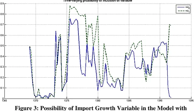
Growth of goods & services imports va2
Economic growth va3
Growth of M1 va4
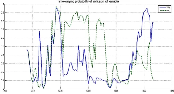
Growth of visible deposits va5
Growh of invisible deposits va6
Variations of market exchange rate (informal exchange rate)
va7
Variations of banks’ deposits va8
model and variable input for modeling and forecasting inflation from inflation in the economy of Iran at any given time series:
Table2: Presented Variables at any Time in Best Model
Period Variable Name Second constant ARY_1 va1_0 va3_0 va8_1 Third constant ARY_1 va1_0 va3_0 va8_1 Fourth constant ARY_1 va1_0 va2_0 va3_0 va5_0 va7_0 va3_1 va6_1 va7_1 2010 First constant ARY_1 va1_0 va2_0 va3_0 va5_0 va7_0 va3_1 va6_1 va7_1 Second constant ARY_1 va1_0 va3_0 va5_0 va7_0 va2_1 va7_1 Third constant ARY_1 va1_0 va3_0 va5_0 va7_0 va2_1 va7_1 Fourth constant ARY_1 va1_0 va2_0 va3_0 va5_0 va7_0 va3_1 va6_1 va7_1 2011 First constant ARY_1 va1_0 va2_0 va3_0 va5_0 va7_0 va3_1 va6_1 va7_1 Second constant ARY_1 va1_0 va2_0 va3_0 va5_0 va7_0 va3_1 va6_1 va7_1 Third constant ARY_1 va1_0 va2_0 va3_0 va5_0 va7_0 va3_1 va6_1 va7_1 Fourth constant ARY_1 va1_0 va2_0 va3_0 va5_0 va7_0 va3_1 va6_1 va7_1 2012 First constant ARY_1 va1_0 va3_0 va5_0 va1_1 va2_1 va3_1 va5_1 va6_1 va7_1 Second constant ARY_1 va1_0 va3_0 va8_1 Third constant ARY_1 va1_0 va3_0 va5_0 va7_0 va2_1 va3_1 Fourth constant ARY_1 va1_0 va3_0 va5_0 va7_0 va2_1 va3_1
In Figure1 the possibility that DMS is the best model at any point of time is presented.
Figure1: Possibility of the Best Model
Given that after the estimate of DMA model, it is possible to determine probable input of independent variables (and intervals) in a simulated inflation is Iran. Figure (2) to (9) shows the possibility of any of the independent variables in the model when it is estimated with the forecast horizon 1 (h = 1).
Figure 2: Possibility of Export Growth in the Model with Prediction Horizon of 1
Figure 4: Possibility of Economic Growth Variable in the Model whit Prediction Horizon of 1
Figure 5: Possibility of M1 Growth in the Model with Prediction horizon of 1
Figure 7: Possibility of Invisible Deposits Growth in the Model with Prediction Horizon of 1
Figure 8: Possibility of Informal Exchange Rate in the Model with Prediction Horizon of 1
According to Figures (2) to (9) the possibility of currency in circulation growth, economic growth, growth in visual and non-visual deposits in modeling of inflation in the economy is more:
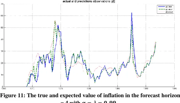
The true and expected value of inflation in the forecast horizon h = 1 and h = 4 with 𝛼 = 𝜆 = 0.99 can be seen in Figures (10) and (11):
Figure 10: The true and expected value of inflation in the forecast horizon h = 1 with 𝜶 = 𝝀 = 𝟎. 𝟗𝟗
Figure 11: The true and expected value of inflation in the forecast horizon h = 4 with 𝜶 = 𝝀 = 𝟎. 𝟗𝟗
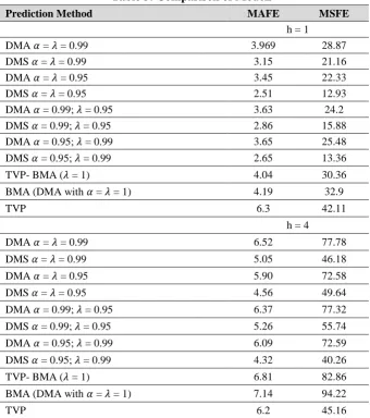
Table 3: Comparison of Models
MSFE MAFE
Prediction Method
h = 1
28.87 3.969
DMA 𝛼 = 𝜆 = 0.99
21.16 3.15
DMS 𝛼 = 𝜆 = 0.99
22.33 3.45
DMA 𝛼 = 𝜆 = 0.95
12.93 2.51
DMS 𝛼 = 𝜆 = 0.95
24.2 3.63
DMA 𝛼 = 0.99; 𝜆 = 0.95
15.88 2.86
DMS 𝛼 = 0.99; 𝜆 = 0.95
25.48 3.65
DMA 𝛼 = 0.95; 𝜆 = 0.99
13.36 2.65
DMS 𝛼 = 0.95; 𝜆 = 0.99
30.36 4.04
TVP- BMA (𝜆 = 1)
32.9 4.19
BMA (DMA with 𝛼 = 𝜆 = 1)
42.11 6.3
TVP
h = 4
77.78 6.52
DMA 𝛼 = 𝜆 = 0.99
46.18 5.05
DMS 𝛼 = 𝜆 = 0.99
72.58 5.90
DMA 𝛼 = 𝜆 = 0.95
49.64 4.56
DMS 𝛼 = 𝜆 = 0.95
77.32 6.37
DMA 𝛼 = 0.99; 𝜆 = 0.95
55.74 5.26
DMS 𝛼 = 0.99; 𝜆 = 0.95
72.59 6.09
DMA 𝛼 = 0.95; 𝜆 = 0.99
40.26 4.32
DMS 𝛼 = 0.95; 𝜆 = 0.99
82.86 6.81
TVP- BMA (𝜆 = 1)
94.22 7.14
BMA (DMA with 𝛼 = 𝜆 = 1)
45.16 6.2
TVP
Source: Research Findings
taking into account the dynamic models in the modeling of inflation, rather than using constant inputs to the model.
5. Conclusion
Inflation forecast is one of the tools in targeting inflation by the central bank. The most important problem that previous models had in forecasting was that were they could not correctly predict over time. However, the central bank policymakers should ignore the short-term and transient changes in prices and seek to create economic stability by estimating constant inflation. Accordingly, in this study, it has been tried to present nonlinear dynamic models for simulation of inflation in Iran’s economy using TVP-DMA and TVP-DMS models. These models can provide the changes in input variables over time as well as changes in the coefficients of variables over time. The results of DMS estimation model represented the input variables have change over time, and the importance of taking into account the dynamic models in the modeling of inflation, rather than using constant input variable.
References
Ball, L., & Mazumder, S. (2011). Inflation Dynamics and the Great Recession. Brookings Papers on Economic Activity, 42(1), 337-405. Cogley, T., Morozov, S., & Sargent, T. (2005). Bayesian Fan Charts for U.K inflation: Forecasting and Sources of Uncertainty in an Evolving Monetary System. Journal of Economic Dynamics and Control, 29, 1893-1925.
Cremers, K. (2002). Stock Return Predictability: A Bayesian Model Selection Perspective. Review of Financial Studies, 15, 1223-1249. Friedman, M. (1968). The Role of Monetary Policy. American Economic Review, 58, 1-17.
Garratta, A., Mitchellb, J., Vahey, S. V., & Wakerly, E. C. (2011). Real-time Inflation Forecast Densities from Ensemble Phillips Curves. North American Journal of Economics and Finance,22, 78-88. Groen, J., Paap, R., & Ravazzolo, F. (2009). Real-time Inflation Forecasting in a Changing World. Erasmus University Rotterdam, Econometric Institute Report, Retrieved from
https://www.econstor.eu/bitstream/10419/60913/1/622767062.pdf. Hamilton, J. (1989) A New Approach to the Economic Analysis of Nonstationary Time Series and the Business Cycle. Econometrica, 57, 357-384.
Hoogerheide, L., Kleijn, R., Ravazzolo, F., van Dijk, H., & Verbeek, M. (2010(. Forecast Accuracy and Economic Gains from Bayesian Model Averaging using Time-Varying Weights. Journal of Forecasting, 29(1-2), 251-269.
Kalman, R. (1960). A New Approach to Linear Filtering and Prediction Problems. Journal of Basic Engineering, 82 (Series D), 35-45.
Koop, G., & Korobilis, D. (2012). Forecasting Inflation Using Dynamic Model Averaging. International Economic Review, 53, 867-886.
Koop, G., & Potter, S. (2004). Forecasting in Dynamic Factor Models using Bayesian Model Averaging. The Econometrics Journal, 7, 550-565.
Lucas, R. Jr. (1976). Econometric Policy Evaluation: A Critique. Carnegie-Rochester Conference Series on Public Policy, Elsevier, 1(1), 19-46.
Moser, S., & Rumler, F. (2007). Forecasting Austrian Inflation. Economic Modeling,24, 470-480.
Nakajima, J., Munehisa, K., & Toshiaki, W. (2011). Bayesian Analysis of Time-varying Parameter Vector Autoregressive Model for the Japanese Economy and Monetary Policy. Journal of the Japanese and International Economies, 25(3), 225-245.
Primiceri, G. (2005). Time Varying Structural Vector Auto regressions and Monetary Policy. Review of Economic Studies, 72, 821-852.
Raftery, A., Karny, M., & Ettler, P. (2010). Online Prediction under Model Uncertainty via Dynamic Model Averaging: Application to a Cold Rolling Mill. Technimetrics, 52, 52-66.
Raftery, A., Karny, M., Andrysek, J., & Ettler, P. (2007). Online Prediction under Model Uncertainty via Dynamic Model Averaging: Application to a Cold Rolling Mill. University of Washington, Technical Report 525, Retrieved from
https://www.tandfonline.com/doi/abs/10.1198/TECH.2009.08104. Stock, J., & Watson, M. (2008). Why Has U. S. Inflation Become Harder to Forecast? Journal of Monetary Credit and Banking, 39, 3-33.