Volume 3, Issue 3, March 2014
Page 147
Abstract
This paper establishes a linkage between a weighted flow-shop scheduling system with a Queue-network in which a common service channel is linked in series with each of two parallel biserial service channels. Where weight of a job shows the relative priority over some other job in a schedule of jobs and in queue-network, it is assumed that the arrival & service pattern in the system both follow Poisson distribution. The objective of the paper is twofold- one to minimizes the weighted mean flow time of two machines and the other, to determines the total waiting times of jobs/items for the optimal sequence of jobs/items in a given queue network model, when items/jobs are processed in a combined system that has the practical utility in the industries, where production is done in such complex stages. A heuristic algorithm is derived and made clear through a numerical illustration.
Keywords: Queue-network, Poisson- process, waiting time, mean queue length, Biseries, weighted flow-shop.
1.
I
NTRODUCTIONSo far the survey of scheduling and queuing theory is concerned; we find a lot of work is being done separately in these fields (Johnson [1954], Jackson [1954], Ignall and Scharge [1965], Maggu [1970], and Singh T.P. [1986] etc.), very little work is found to deal with combining operation of these two systems. Johnson [1954] gave polynomial time scheduling algorithm to minimize the total idle time of machines in two stage flow-shop scheduling. Maggu [1970] studied a network of two queues in biseries finding the total idle times of items/customers. Maggu & Dass [1985] introduce the concept of weight for the jobs in flow-shop scheduling. Singh T.P.etal [1986, 2005, 2006] studied the behavioral aspect of various types of queue and scheduling system of practical importance under different parameters. Further Singh T.P. & Kumar Vinod [2005, 2006] studied the transient and steady-state behaviour of biserial channels linked with a common channel. Singh T.P. & Kumar Vinod [2008] deals the combining operation to a scheduling system with a network of queuing system in series.
Recently, Singh T.P. & Kumar Vinod [2009, 2010] made an attempt to continue the idea of combining operation to a scheduling system with a biserial queuing network in wider aspect.
This paper is further an extension of the study made by Singh T.P. & Kumar Vinod [2009, 2010] and establishes a linkage between a network of weighted flow-shop processing the jobs with a queue network in biseries which are linked to a common channel. Thus the paper makes a bridge between the two-stage scheduling system given by Johnson [1954] with weighted flow-shop system introduced by Maggu & Dass [1985] on one side, and on other side a network of queue model given by Kumar Vinod & Singh T.P. [2005, 2006].
2.
A
SSUMPTIONS1. Each jobs is processed in the prescribed order M1, M2, ---, Mm i.e. a flow-shop, also no passing of jobs is permitted.
And a machine can process only one job at a time.
2. Let Mij denote the processing time of job Ji on Mj. Set up times for operations are sequence-independent and are
included in the processing times.
3. Each job is assigned weight wi according to its importance.
4. Let Fj (i) denote the partial flow-time of Ji counted from the starting time of first job J1 on M1, in particular, Fm (i) is
called as flow-time of Ji.
5. The performance measure is weighted mean flow-time defined by-
n
1 i
i n
1 i
m i
w
w (i) F w
F
6. We assume that the effective arrival rate at the first queue in the model follows Poisson distribution.
7. The weighted mean flow-time in the optimal schedule of the items process through the machines formed the mean arrival rate at the first service channel in the queue network model.
8. For the existence of steady-state behaviour following condition is hold-
On Linkage of A Weighted Flow-Shop
Scheduling System with Biserial Queue
Network
Vinod Kumar Kakoria
Volume 3, Issue 3, March 2014
Page 148
λ < µi ; (i = 1,2,---) i.e.i λ ρ
μ
< 1
Where λ : Mean arrival rate. µi : Mean service rate. ρ : Utility factor.
3.
P
RACTICALS
ITUATIONWe can consider a network of such weighted flow-shop system in a Production concern in which the machines are linked serially with a network of queues comprised of three service channels, one of them is commonly linked in series with each of other two servers in biseries. Let us suppose, there are machines for grinding & finishing. The jobs/items which are stored in godown with relative priority over some other jobs/items after grinding & finishing on the machines enter to the queue system and join any server without condition (i.e. they can join any server first out of the two biserial servers and then join the second) for the two types of labeling (one is for Company Mark & other is for the Product Name) on the product. After labeled both the label, items/jobs go to the third common server for O.K- Testing. Finally after completing the service items/jobs goes out from the network.
4.
M
ATHEMATICALM
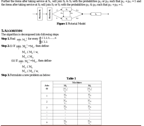
ODELINGConsider a network of weighted flow-shop system n-jobs × 2-machine M1 & M2 linked serially with a network of queues
comprised of three service channels S1, S2 & S3, where S3 is commonly linked in series with each of two servers in
biseries S1 & S2. Queues Q1, Q2 & Q3 are formed in front of the servers S1, S2 & S3, if they are busy. It is to be assumed
that the output weighted mean flow-time of jobs in the optimal sequence follows Poisson law. Also the weighted mean flow-time of these jobs in the optimal sequence of the jobs form the effective average arrival rate = λ Here items/jobs after getting optimal sequence may join either the queue Q1 or Q2 with the probabilities p & q respectively such that p + q = 1.
Further the items after taking service at S1, will join S2 & S3 with the probabilities p12 or p13 such that p12 + p13 = 1 and
the items after taking service at S2 will join S1 or S3 with the probabilities p21 & p23 such that p21 + p23 = 1.
Figure 1 Pictorial Model
5.
A
LGORITHMThe algorithm is decomposed into following steps:
Step 1. Find
ij j
min M for every i 1, 2,3,..., n j 1, 2.
Step 2. (i) If
ij j
min M =Mi1, then define-
'
i1 i1 i '
i 2 i2
M M w
M M
(ii) If
ij
jmin M =M , then define- i2 '
i1 i1
'
i 2 i 2 i
M M
M M w
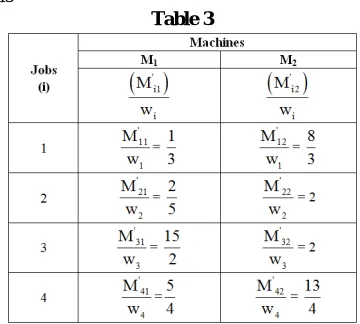
Step 3. Formulate a new problem as below:
Volume 3, Issue 3, March 2014
Page 149
Step 4. Find optimal sequence by using Johnson [1954] algorithm for the reduced problem in step-3. This will be optimal or near to optimal for the original problem minimizing the weighted mean flow-time.
Step 5. Find weighted mean flow-time for the optimal sequence obtained in step-4 by using the formula-
n
1 i
i n
1 i
m i
w
w (i) F w F
Step 6. The weighted mean flow-time
F
w obtained in step-5 is the mean arrival rate λ for the queue network .Step 7. Apply Mean queue length formula for the steady-state system given by Singh T.P. & Kumar Vinod [2005, 2006], which is as-
2
12 21
2 1 12
12 1 2
21 2 1 21 12 1
21 2 1
p
λ λ
p p 1
μ
p
λ λ
p
λ λ
p p 1
μ
p
λ λ
L
12 21
13
1 2 21
23
2 1 12
312 1 2 23 21 2 1 13
p
λ λ
p p
λ λ
p p p 1
μ
p
λ λ
p p
λ λ
p
The steady-state equations of the system exist under the assumptions-
(i)
12 21
1
21 2 1
p p 1 μ
p λ λ
< 1
(ii)
12 21
212 1 2
p p 1 μ
p λ λ
< 1
(iii)
12 21
3
12 1 2 23 21 2 1 13
p p 1 μ
p λ λ p p λ λ p
< 1
Where λ1= λp, λ2= λq s.t. p + q = 1
Step 8. Find the Waiting time for the customer by using well-known Little’s [1961] formula-
λ L W
6.
N
UMERICALI
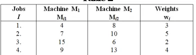
LLUSTRATIONConsider four jobs are processed through the network of two machines M1 & M2 in this order with processing time Mij
and weight wi of job i on machine j given as-
Table 2
Let this scheduling system is linked with a network of three queues Q1, Q2 & Q3 with the service channels S1, S2 & S3,
where S3 is commonly linked in series with each of two servers in biseries S1 & S2. Let µ1 = 25, µ2 = 30 & µ3 = 40 be the
mean service rate for the service channels S1,S2 & S3respectively, where λ is the arrival rate of items/jobs and remember
λ < µ1, λ < µ2and λ < µ3. Let p = 0.45 & q = 0.55 be the probabilities of joining the items/jobs after getting optimal
sequence to queues Q1 & Q2 respectively such that p + q = 1, and p12 = 0.3 & p13 = 0.7 be the probabilities of joining the
items/jobs to queues Q2 & Q3 after taking service at S1 such that p12 + p13 = 1. Similarly p21 = 0.6 & p23 = 0.4 be the
probabilities of joining the items/jobs to queues Q1 & Q3 after taking service at S2 such that p21 + p23 = 1.
Our objective is to find the mean queue length and waiting time of the customers/items in this linkage problem.
6.1 Solution
As per step-1, Find
ij
j
min M
for every i 1, 2, 3,..., n j 1, 2.
min (M11, M12) = min (4, 6) = 4
min (M21, M22) = min (7, 10) = 7
min (M31, M32) = min (15, 6) = 6
min (M41, M42) = min (9, 13) = 9
Volume 3, Issue 3, March 2014
Page 150
M’11= M11 – w1 = 4 – 3 = 1 M’12= M12 = 8M’21= M21 – w2 = 7 – 5 = 2 M’22= M22 = 10
M’32= M32 + w3 = 6 + 2 = 8 M’31= M31 = 15
M’41= M41 – w4 = 9 – 4 = 5 M’42= M42 = 13 As per step-3, The reduced problem is-
Table 3
As per step-4, using Johnson’s algorithm we get the optimal sequence as- (1, 2, 4, 3)
As per step-5, the completion time for the optimal sequence obtained in step-1 is-
Table 4 Jobs
(i)
Machine M1
in -- out
Machine M2
in -- out
1. 2. 4. 3.
00 --- 04 04 --- 11 11 --- 20 20 --- 35
04 --- 08 11 --- 21 21 --- 34 35 --- 41
F2 (1) = 8, F2 (2) = 21, F2 (4) = 34, F2 (3) = 41.
Hence weighted mean flow-time
F
w for the schedule (1, 2, 4, 3) is- 4i 2 i 1 w 4
i i 1
w F (i) F
w
= 1 2 2 2 4 2 3 2
1 2 4 3
w F (1) w F (2) w F (4) w F (3)
w w w w
2 4 5 3
41 2 34 4 21 5 8 3
14 347
=24.79
As per step-6, find the effective average arrival rate λ as-
w
F
λ
= 24.79As per step-7, find Mean queue length by using the formula-
2
12 21
2 1 12
121 2
21 2 1 21 12 1
21 2 1
p λ λ p p 1 μ
p λ λ p
λ λ p p 1 μ
p λ λ L
12 21
13
1 2 21
23
2 1 12
3
12 1 2 23 21 2 1 13
p λ λ p p λ λ p p p 1 μ
p λ λ p p λ λ p
Here, p = 0.45, q = 0.55, λ = 24.79 and µ1 = 25, µ2 = 30, µ3 = 40
λ1= λp = 24.79 × 0.45 = 11.16 and λ2= λq = 24.79 × 0.55 = 13.63
p12 = 0.3 p13 = 0.7 p21 = 0.6 p23 = 0.4
1 0.3 0.6
13.63
11.16 0.3
30
0.3 6 1 . 1 1 63 . 3 1 0.6
63 . 3 1 6 1 . 1 1 0.6 0.3 1 25
0.6 63 . 3 1 6 1 . 1 1 L
Volume 3, Issue 3, March 2014
Page 151
1 0.3 0.6
0.7
11.16
13.63 0.6
0.4
13.63
11.16 0.3
400.3 6 1 . 1 1 63 . 3 1 0.4 0.6 63 . 3 1 6 1 . 1 1 0.7
30
0.82
13.63 3.348
348 3. 63 . 3 1 178
. 8 6 1 . 1 1 0.82 25
178 . 8 6 1 . 1 1
0.82
0.7
11.16 8.178
0.4
13.63 3.348
40348 3. 63 . 3 1 0.4 178 . 8 6 1 . 1 1 0.7
978 . 6 1 24.6
978 . 6 1 338 . 9 1 20.5
338 . 9 1
+
13.53 6.79
32.8
79 6. 53 . 3 1
=
162 . 1
338 . 9
1 +
22 .6 7
78 .9 6 1
+
48 . 2 1
32 . 20
= 16.64 + 2.22 + 1.63 = 20.49
As per step-8, find Total waiting time of a customer using the Little’s [1961] formula as- L
W λ
=
79 . 4 2
49 0. 2
= 0.826
7.
R
EMARKS1. If the concept of weights to the jobs in 1st phase is not taking in to account, the result of the paper resemble with [2009].
2. This study is wider and more applicable comparatively to the study made by [2008, 2009, and 2010].
3. L & W are the decision making parameters which are helpful to the managers in an organization to find better decision for the relevant problems in such a complex system.
References
[1] S.M. Johnson [1954]: “Optimal two & three stage production schedule with set-up times included”. Nav Res Log. Quartz. Vol.1 pp 61-68
[2] Jackson. R. R.P.[1954] : “Queuing system with phase type service”. O.R. Quatz. Vol. 5,No. 4, pp 109-120.
[3] Little John D.C. [1961]: “A Proof for the Queuing Formula: L = λW” Operations Research, Vol. 9, No. 3 (May-Jun., 1961), pp. 383-387.
[4] Ignalle., and Schrage, L. [1965] “Application of the branch-and bound technique to some flow shop scheduling problems”. Operation Research, 13,400-412.
[5] Maggu.P.L. [1970]: “Phase type service queues with two servers in Biseries”. J.Op.Res.Sco. Japan Vol.13, No.1.
[6] Maggu.P.L. & Dass G. [1985]: “Elements of Advanced Production Scheduling”. United Publishers and Periodical Distributors, New Delhi, pp 105-111.
[7] Singh T.P. [1986]: Ph.D.Thesis “On some networks of Queuing & Scheduling System” Garhwal University Shrinagar Garhwal.
[8] Singh T.P., Kumar Vinod & Kumar Rajender [2005]: “On trasient behaviour of a queuing network with parallel biserial queues”.JMASS Vol. 1 No. 2, December. pp 68-75.
[9] Singh T.P., Kumar Vinod & Kumar Rajender [2006]: “Steady-state behaviour of a network of queue comprised of two sub-systems with heterogeneous channels linked in series with a common channel”. Reflection des ERA Vol.1,Issue 2,May. pp 135-52.
[10] Maggu.P.L. & Gupta Shameena [2006]: “On a network of two queues in bitandem linked in series with a network of two machines in flow-shop” JISSOR, Vol. XXVII, No.1-4 Dec 2006, pp 11-15.
[11] Singh T.P., Kumar Vinod & Kumar Rajender [2008]: “Linkage of Scheduling system with a serial Queue-network” Lingaya’s Journal of Professional Studies, Vol. 2, No. 1 July-Dec.,2008. pp. 25-30.
[12] Singh T.P., & Kumar Vinod [2009]: “On Linkage Of Scheduling System With A Biserial Queue-Network” Arya Bhatta Journal Of Mathematics & Informatics, Vol. 1, No. 1-2 July-Dec., 2009. pp. 71-76. and Presented in National Conference of ISITA on Challenges in Software Engg. Research & Practices from 30-31 March, 2010.