Volume 2007, Article ID 97278,18pages doi:10.1155/2007/97278
Research Article
Modification of the Quasilinearization Method
for the Inverse Problem
Lenka ˇ
Celechovsk´a-Koz´akov´a
Received 25 January 2006; Revised 30 May 2006; Accepted 7 December 2006
Recommended by Virginia Kiryakova
We propose a new modification of Bellman’s quasilinearization method such that at any iteration step, it works with an approximate solution of the original nonlinear system and with new approximation of parametersα(k+1)which are close enough to the previous ones. As an output, this approach provides a construction of a convergent sequence of parameters where the limit is the best approximation of parameters of a given system. We apply this method to a mathematical model describing BSP-kinetics in the human liver.
Copyright © 2007 Lenka ˇCelechovsk´a-Koz´akov´a. This is an open access article distributed under the Creative Commons Attribution License, which permits unrestricted use, dis-tribution, and reproduction in any medium, provided the original work is properly cited.
1. Introduction
For solving the inverse problems, in particular, for identification of systems with known structure, the quasilinearization method (QM) is a standard tool. Designed by Bellman et al. [1], this method was later applied to different kinds of identification problems (cf. [2] or [3] for references). We were interested in application of QM to solve the parameter identification problem for the BSP-kinetics in the human liver [4–7]. One of the possible descriptions of this kinetics can be given by the nonlinear system of ordinary differential equations
˙
X(t)= −c1X
K1−Y
, ˙
Y(t)=c1X
K1−Y
−c2Y
K2−Z
, ˙
Z(t)=c2Y
K2−Z
−c3Z,
(1.1)
Table 1.1. The amount of BSP in the blood.
[image:2.468.53.414.142.228.2]Time (min) ti 0 3 5 10 20 30 43 BSP (mg) ri=X(ti) 250 221 184 141 98 80 64
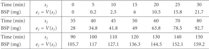
Table 1.2. The amount of BSP in the bile.
Time (min) sj 0 5 10 15 20 25 30 BSP (mg) ej=V(sj) 0 0.2 2.5 6 10.5 15.8 21.7 Time (min) sj 35 40 45 50 60 70 80 BSP (mg) ej=V(sj) 28 34.8 41.8 49 63.8 78.5 92.7 Time (min) sj 90 100 110 120 130 140 150 BSP (mg) ej=V(sj) 105.7 117 127.1 136.3 144.5 152.1 159.2
(mg) of BSP is injected into the blood at once. This leads to the initial conditions
X(0)=I, Y(0)=Z(0)=0. (1.2)
In order to uniquely determine the unknown positive parametersα=(K1,K2,c1,c2,c3), we have to know at least two different data sets. From practical point of view, we can ob-tain data describing the decreasing level of BSP in the blood (Table 1.1) and inTable 1.2, they are presenting the measurements of BSP in the bile. These data were obtained through medical experiments by Hrnˇc´ıˇr [6].
The first data set corresponds to the functionX(t). The second one corresponds to the functionV(t)=I−X(t)−Y(t)−Z(t) describing the level of BSP in the bile.
However, the standard approach like in [2,3], or recent [8,9] does not provide the reasonable outputs corresponding to the nature of parameters, especially if we solve an identification problem for nonlinear system of ordinary differential equations. (We can obtain negative values of determinated parameters, seeSection 5.) Therefore we propose a modification of the quasilinearization method (MQM). The algorithm of the modified QM consists of the steps displayed below. Let us briefly introduce the MQM (seeSection 3 for details).
Step 1. Consider a nonlinear autonomous initial problem
˙
x=f(x,α), x(0)=c,
wherex∈Rn,α∈RN, andf:Rn+N→Rnis a continuous function. This problem is equivalent to the Cauchy problem
˙x=g(x), x(0)=c,
where
x=(x,α)=x1,. . .,xn,α1,. . .,αN
∈Rn+N,
g(x)=
f(x,α), 0,. . ., 0
N ,
c=c1,. . .,cn,β1,. . .,βN∈Rn+N.
Step 2. Choose the initial approximationα(1), the toleranceε >0, and putk=1.
Step 3. Compute the solution x(k)(t) of the system
˙x(t)=g(x),
with the initial condition
x(0)=c1,. . .,cn,α1(k),. . .,α(Nk)
.
Step 4. Evaluate the solution y(k+1)(t) of the linearized equation in a particular form
y(k+1)(t)=p(k+1)(t) +
N
j=1
βjh(j,k+1)(t).
Step 5. Determine the minimumβ∗of the penalty functionΨ
k+1(β) :=Υ(y(k+1)) and set
α(k+1):=β∗.
Step 6. Chooseζk>0, that is, the maximum allowed distance between the parametersα(k+1)and
α(k).
Step 7. If the deviationS(x(k+1))< S(x(k)) and
(a)α(k+1)−α(k) ≤ζ
k, then go toStep 3; (b)α(k+1)−α(k)> ζ
k, then suitably change the valueα(k+1)(seeLemma 3.5for details).
Step 8. Setk:=k+ 1 and repeat Steps3,4,5,6,7(a), respectively,Step 7(b) until the condition
0≤Sx(k)−Sx(k+1)< ε
is satisfied.
Step 9. IfS(x(k+1))> S(x(k)), then go back toStep 2and start the algorithm with a better choice
α(1).
parameters is reached (according to the criteria for stopping the computatuion given in Steps8-9).
The organization of this paper is as follows. InSection 2we give a basic notations and definitions. InSection 3we describe the modification of quasilinearization method in de-tail, and inSection 4we give the convergence theorem.Section 5includes the numerical results.
2. Notations and definitions
LetRmbe a vector space with the scalar product
(u,v) :=uv=
m
i=1
uivi, (2.1)
u=(u1,. . .,um)∈Rm,v=(v1,. . .,vm)∈Rm. The associated norm is
u:=(u,u)1/2. (2.2)
LetA=(ai j),i,j=1,. . .,m, be anm×mmatrix. Then the matrix norm is given by
A:=
m
i,j=1
ai j2 1/2
. (2.3)
The matrixAis called positive definite if there is a constantK >0 such that
(u,Au)≥Ku2 (2.4)
for everyu∈Rm.
Lemma 2.1. Letγ=(γ1,. . .,γm)∈Rm. LetMbe anm×msymmetric matrix of the form
M=Γ+E, (2.5)
whereΓ=γγ=(Γ1,. . .,Γm),Γi∈Rmfor alli=1,. . .,m, andEis them×midentity
ma-trix. Then the matrixMis positive definite.
Proof. Denote
Mkk=
M1,. . .,Mk
=
⎛ ⎜ ⎜ ⎜ ⎝
m11 ··· m1k ..
. . .. ...
mk1 ··· mkk
⎞ ⎟ ⎟ ⎟
⎠. (2.6)
We can write the matrixMkkin the form
Mkk=
Γ1+e1,. . .,Γk+ek
whereei=(0,. . ., 0, 1, 0,. . ., 0)is the k-dimensional vector with 1 on the ith position,
i=1,. . .,k. The minor detMkkof the matrixMcan be evaluated as follows:
detMkk=det
Γ1+e1,. . .,Γk+ek
= ···
=detE+ k
l=1
dete1,. . .,el−1,Γl,el+1,. . .,ek
+ 2k−k−1
j=1
detQj,
(2.8)
whereQjare the matrices with at least two columnsΓr,Γs. Thesek-dimensional vectors
Γr,Γsare not linearly independent since
Γi=γiγ=γi
γ1,. . .,γk
, γi∈R, (2.9)
for alli=1,. . .,k. Therefore,
detMkk=detE+ k
l=1
det(e1,. . .,el−1,Γl,el+1,. . .,ek)=1 + k
l=1
γ2l, (2.10)
and the matrixMis positive definite by Sylvester criterion [10, page 248].
Lemma 2.2. Let M be anm1×m1symetric positive definite matrix of the form (2.5). LetE
bem2×m2identity matrix. Letm=m1+m2. Then the block diagonalm×mmatrix
Md=
⎛
⎝M 0
0 E
⎞
⎠ (2.11)
is positive definite too.
The proof is clear.
Lemma 2.3. LetL2
m[0,T] be the space of vector functionsh(t)=(h1(t),. . .,hm(t))with the scalar product
(h,g)=
T
0
h(t),g(t)Rmdt. (2.12)
Let the matrixMd have the form (2.11). Then
h,g =
T
0
h(t)Mdg(t)dt (2.13)
is a scalar product onL2
m[0,T] too.
The proof follows easily byLemma 2.2.
Remark 2.4. There are norms ofm-dimensional vector functionh(t),
h2=(h,h), (2.14)
|h|2
= h,h, (2.15)
Lemma 2.5. LetCm[0,T] be the normed space of continuousm-dimensional vector functions with the norm
hC= max t∈[0,T]
h(t)
Rm. (2.16)
If the sequence of functions{hn(t)}∞n=1 is uniformly convergent to the functionh(t) in the
spaceCm[0,T], that is, lim
n→∞hn−hC=0, then
lim
n→∞hn−h=0, (2.17)
where the normhis defined by (2.14).
Proof. We can write
hn−h2
=hn−h,hn−h
=
0
hn(t)−h(t),hn(t)−h(t)
Rmdt
≤
0 tmax∈[0,T]
hn(t)−h(t),hn(t)−h(t)
Rmdt
=
0 tmax∈[0,T]
hn−h2 Rmdt=
0
hn−h2 Cdt
=Thn−h2C.
(2.18)
Hence
√
Thn−hC≥hn−h. (2.19)
From this inequality, the assertion ofLemma 2.5follows.
LetD⊂Rmbe a convex set. The functionS:D→Ris called a strictly convex function if there is a constantχ >0 such that for everyu,v∈Dand for everyα∈[0, 1], the inequality
Sαu+ (1−α)v≤αS(u) + (1−α)S(v)−α(1−α)χu−v2 (2.20)
is satisfied. The constantχis called the constant of the strict convexity of the functionSon the setD.
Lemma 2.6. LetD⊂Rmbe a convex closed set. LetS(u) have the form
S(u)=uAu+bu+c, (2.21)
whereAis a positive definitem×mmatrix,b∈Rm, andc∈R. ThenSis a strictly convex
function.
3. Modification of the quasilinearization method
LetQ⊂Rnbe a closed convex set of the variablesx=(x1,. . .,x
n)and letD⊂Rnbe a closed convex set of the parametersα=(α1,. . .,αN). Letf :Q×D→Rnhave continuous bounded partial derivatives up to the second order. Consider a nonlinear autonomous system of ordinary differential equations with the initial condition
˙
x(t)=f(x,α),
x(0)=c. (3.1)
In order to avoid considering two different types of vectors, we will suppose that the vectorαsatisfies the differential equation
˙
α(t)=0 (3.2)
with the initial condition
α(0)=β, (3.3)
whereβ=(β1,. . .,βN). Define a new vector x by
x=(x,α)=x1,. . .,xn,α1,. . .,αN
∈Rn+N, (3.4)
and a vector c (corresponding to the initial condition) by
c=(c,β)=c1,. . .,cn,β1,. . .,βN
∈Rn+N. (3.5)
The vector x(t) satisfies the nonlinear differential equation
˙x(t)=g(x), (3.6)
where g(x)=(f(x,α), 0, . . ., 0
N
), with the initial condition
x(0)=c. (3.7)
The aim is to find the unknown parametersα such that the solution of the initial problem (3.1) fits in some sense with a given toleranceε >0 to the measured data or to the continuous function which approximates these data, respectively.
using spline interpolation. Our motivation is the Cauchy problem given by (1.1), (1.2) described in the intoduction.
The weighted deviation,Γ:Cn[0,T]→R, of a given functionz(t)∈Cn[0,T] from the approximating functionsr(t) ande(t) can be expressed, in sense of the least-square method, in the form
Γ(z)=
n l=1 0
zl(t)−rl(t)2dt
+ 0 γ+ n l=1
γlzl(t) −e(t) 2
dt, (3.8)
whereγ,γlare given real weighting constants (in our case,γ=X(0)=Iandγl= −1 for
l=1, 2, 3).
Lemma 3.1. LetCn[0,T] be the space of continuous vector functionsz(t) with the norm
(2.16), form=n. LetΓ(z) have the form (3.8). ThenΓ(z) is continuous fromCn[0,T] toR.
The proof follows easily byLemma 2.5andRemark 2.4. Let x(k)(t)=(x(k)
1 (t),. . .,x (k)
n (t),α(1k),. . .,α (k)
N )(kth iteration) be a solution to (3.6) on the interval [0,T] with the initial condition (3.7) for c=(c1,. . .,cn,α(1k),. . .,α
(k) N ). The solution of the equivalent system (3.1) forα=α(k)=(α(k)
1 ,. . .,α (k)
N )isx(k)=(x (k) 1 (t),. . .,
xn(k)(t)). The deviation between the solutionx(k)(t) and measured data has the form (3.8), that is,
Sx(k)= n
l=1
0
xl(k)(t)−rl(t)
2 dt + 0 γ+ n
l=1
γlx(lk)(t) −e(t) 2
dt. (3.9)
We would like to find a new vector of parametersβ=α(k+1)so that
Sx(k+1)< Sx(k). (3.10)
The dependence of x(k)(t), respectively,x(k)(t) on the parametersβ(β=α(k)) is not clear, therefore we approximate x(k)(t) by the solution y(k+1)(t) of a linearized system
˙y(t)=gx(k)(t)+ Jx(k)(t)y(t)−x(k)(t), (3.11)
where J(x) is the Jacobian matrix of g(x).
Equation (3.11) is a linear system ofn+N differential equations and its general
solu-tion y(t) with
yj(0)=
⎧ ⎪ ⎨ ⎪ ⎩
cj forj=1,. . .,n,
βj−n forj=n+ 1,. . .,n+N,
(3.12)
can be represented in the form
y(t)=y(k+1)(t)=p(k+1)(t) + N
j=1
Here the function p(k+1)(t) is the (particular) solution of the nonhomogeneous equation
˙p(t)=gx(k)(t)+ Jx(k)(t)p(t)−x(k)(t) (3.14)
which fulfills the initial condition
p(0)=c1,. . .,cn, 0,. . ., 0
, (3.15)
the (n+N)-column vectors h(j,k+1)(t), j=1,. . .,N, are solutions of the homogeneous system
˙h(j,k+1)(t)=Jx(k)(t)h(j,k+1)(t) (3.16)
with
h(ij,k+1)(0)=
⎧ ⎪ ⎪ ⎨ ⎪ ⎪ ⎩
0 fori=n+j,
1 fori=n+j,i=1,. . .,n+N.
(3.17)
Let
H(k+1)(t) :=h(1,k+1)(t),. . ., h(N,k+1)(t) (3.18)
be the (n+N)×Nmatrix with the columns equal to the solutions of (3.16), (3.17). Then the solution (3.13) can be written in the form
y(k+1)(t)=p(k+1)(t) + H(k+1)(t)β, (3.19)
whereβ=(β1,. . .,βN).
Lemma 3.2. Lett∈[0,T]. Let x(k)(t) be the solution to (3.6), (3.7) for x(k)(0)=(c1,. . .,c n,
α(1k),. . .,α (k)
N )and let y(k+1)(t) be the solution to (3.11) with the initial conditions (3.12). If,
moreover,β=α(k), then
y(k+1)(t)=x(k)(t) (3.20)
fort∈[0,T]. This means that
x(k)(t)=p(k+1)(t) + H(k+1)(t)α(k). (3.21)
From the equality (3.13), we can see immediately that the dependence of y(k+1)(t) on the parametersβj,j=1,. . .,N, is affine. The parametersβj,j=1,. . .,N, are free and they can be used for minimizing the functionΥ:Cn+N[0,T]→R,
Υy(k+1)=
0
y(k+1)(t)−r(t)y(k+1)(t)−r(t)dt
+
0
γ+
n
l=1
γlyl(k+1)(t)−e(t) 2
dt,
(3.22)
where r(t)=(r1(t),. . .,rn(t), y(nk+1+1)(t),. . ., y (k+1)
n+N(t)),γ=(γ1,. . .,γn, 0,. . ., 0)∈Rn+N. It is easy to see thatΥ(z1,. . .,zn+N)=Γ(z1,. . .,zn) for allz1,. . .,zn+N∈C[0,T].
Since the functionΥ(y(k+1)) depends onβ, we can look at the functionΥ(y(k+1)) as a function of parametersβ=(β1,. . .,βN). Let
Ψk+1(β) :=Υy(k+1) (3.23)
be the function fromRNtoR.
It is easy to show that the functionΨk+1(β) is a quadratic polynomial in the variables
β1,. . .,βN, that is,
Ψk+1(β)=βAk+1β+bk+1β+ck+1, (3.24)
where the coefficientsAk+1,bk+1,ck+1are as follows:
Ak+1=
0
H(k+1)(t)γγ+EH(k+1)(t)dt (3.25)
is anN×Nmatrix,Eis (n+N)×(n+N) unity matrix,
bk+1=2
0
p(k+1)(t)−r(t)+p(k+1)(t)γγ
+e(t)−γγH(k+1)(t)dt
(3.26)
is anN-dimensional row vector, and
ck+1=
0
γ−e(t)γ−e(t) + 2γp(k+1)(t)+p(k+1)(t)γγp(k+1)(t)
+r(t)−p(k+1)(t)r(t)−p(k+1)(t)dt
(3.27)
is a real constant.
The quadratic polynomial (3.24) is continuously differentiable in the variable β= (β1,. . .,βN), where for the derivatives, we have
Sk+1(β)=2βAk+1+bk+1,
Sk+1(β)=2Ak+1,
and the higher derivatives are zero becauseSk+1is anN×Nconstant matrix. The matrix
Ak+1has the form
Ak+1=
⎛ ⎜ ⎜ ⎜ ⎝
h(1,k+1), h(1,k+1) ··· h(N,k+1), h(1,k+1) ..
. . .. ...
h(1,k+1), h(N,k+1) ··· h(N,k+1), h(N,k+1)
⎞ ⎟ ⎟ ⎟
⎠. (3.29)
The elements of the matrixAk+1are scalar products on the spaceCn+N[0,T] given by (2.13) with the (n+N)×(n+N) symmetric block diagonal matrix
Md=Γ+E=γγ+E. (3.30)
In the following lemma, we give the necessary condition for positive definiteness of the matrixAk+1.
Lemma 3.3. Let h(j,k+1)(t), j=1,. . .,N, be the solutions of (3.16), (3.17). Then the matrix
Ak+1is positive definite.
Proof. MatrixAk+1is the Gramm matrix which is real and symmetric. Since the vectors
h(j,k+1)(t) are linearly independent, we have detA
k+1=0. Letλj,j=1,. . .,N, be the eigen-value of the matrixAk+1and letu(j)be the corresponding eigenvector,u(j) =0. Then
λj∈Rand
0<u(j),u(j)=u(j)A
k+1u(j)=
u(j)λ
ju(j)=λj N
i=1
u(ij)2. (3.31)
This inequality implies that all eigenvalues are positive. There are orthogonal matrixOk+1 and diagonal matrixDk+1=diag(λ1,. . .,λN) so that
Ak+1=Ok+1Dk+1Ok+1. (3.32)
Letβ=(β1,. . .,βN)∈RN,β =0. Then
β,Ak+1β=Ok−1+1β,Dk+1Ok−1+1β
≥min j λj
O−1k+1β,O−1k+1β
=min
j λj(β,β)=minj λjβ
2. (3.33)
In the next lemma, we give a set and its property in which we look for the minimum of the function (3.24).
Lemma 3.4. LetSk+1(β) have the form (3.24). DenoteVk:=S(x(k)), wherex(k)is a solution
of (3.1) forα=αk. Define
Mαk:= β|β∈D,Ψk+1(β)≤Vk !
. (3.34)
Proof. Letβ1,β2∈Mαk,a∈(0, 1). DenoteA=Ak+1,b=bk+1ac=ck+1. Then
Ψk+1aβ1+ (1−a)β2=aβ1+ (1−a)β2Aaβ1+ (1−a)β2+baβ1+ (1−a)β2+c =a2β
1Aβ1+2a(1−a)β1Aβ2+(1−a)2β2Aβ2+abβ1+(1−a)bβ2+c =aβ1Aβ1+abβ1+ac+ (1−a)β2Aβ2+ (1−a)bβ2+ (1−a)c
+ 2a(1−a)β1Aβ2−a(1−a)β1Aβ1−a(1−a)β2Aβ2 ≤aVk+ (1−a)Vk−a(1−a)
β1−β2
Aβ
1−β2
≤Vk.
(3.35)
The last inequality holds sinceAis positive definite.
The necessary conditions for determining the local extreme on the setMαk are given
by the equations
∂Ψk+1(β)
∂βj =
0, j=1,. . .,N. (3.36)
Let us denote the solution of (3.36) byβ∗=(β∗1,. . .,β∗N). Since the matrixAk+1is pos-itive definite byLemma 3.3and the functionΨk+1(β) is the strictly convex function by Lemma 2.6,β∗is the unique point of minimum (see [11, page 186]). Put
α(k+1):=β∗=β∗ 1,. . .,β∗N
.
(3.37)
In this way, we obtain new initial condition
x(k+1)(0)=c,α(k+1) (3.38)
for the solution x(k+1)(t) of (3.6). Computing this solution, we get the solutionx(k+1)of the equivalent system (3.1) forα=α(k+1). Determine the deviation (3.9). If the inequality (3.10), that is,
Sx(k+1)< Sx(k), (3.39)
holds and the distance betweenα(k)andα(k+1)is small, that is,
α(k+1)−α(k)≤ζ
k, (3.40)
for a givenζksmall, then we can repeat the whole process of enumeration until the con-dition
0≤Sx(k)−Sx(k+1)< ε, (3.41)
whereε >0 is a given tolerance, is satisfied. If the inequality (3.10) is fulfilled, but
α(k+1)−α(k)≥ζ
we have to modify the value of the parameterα(k+1). The modification is based on the following lemma.
Lemma 3.5. LetMαkhave the form (3.34) (cf.Lemma 3.4). Then for arbitraryζk>0, there
is a parameterα(k+1)∈M
αksuch that
α(k+1)−α(k)≤ζ
k. (3.43)
Proof. Letβ∗∈Mαkbe an argument of minima ofΨk+1(β). SinceMαkis a convex set, we
can look for the parameterα(k+1)in the form
α(k+1)=(1−a)α(k)+aβ∗, (3.44)
wherea∈(0, 1). The object is to find a proper valueasuch that the vectorα(k+1)has to satisfy the inequality (3.43). We would like to have
α(k+1)−α(k)=(1−a)α(k)+aβ∗−α(k)=aβ∗−α(k)≤ζ
k. (3.45)
Hence, we have to chooseasuch thata≤ζk/β∗−α(k).
We are able to shift the parameterα(k+1)toα(k)such that the distance betweenα(k+1) andα(k)is arbitrarily small, in particular less than a given toleranceζ
k.
IfS(x(k+1))> S(x(k)) (the value of deviation has increased), we have to stop the whole process of computation and to start with a better choice of the initial approximationα(1). IfS(x(k+1))=S(x(k)) holds, we get the required values of parametersα=α(k)and the algorithm cannot produce better parameter values (for a givenα(1)) and we are finished.
In the following lemmas, we describe the changes of the distance between the functions x(k)(t), x(t) and between x(k)(t), y(k+1)(t).
Lemma 3.6. Let x(k)(t), x(t) be the solutions of (3.6), with the initial condition x(k)(0)=
(c,α(k)), x(0)=(c,α). Then for anyζ >0, there isζ
k>0 such that
x(k)−x
C≤ζ, (3.46)
whenever
α(k)−α≤ζ
k. (3.47)
Proof. The proposition follows from the continuous dependence of the solution x(t) of
(3.6) on the initial conditions [12, page 94].
Corollary 3.7. Let the functionS(z) have the form (3.8). Let x(k)(t), x(t) be the solutions
of (3.6), with the initial conditions x(k)(0)=(c,α(k)), x(0)=(c,α). Letx(k)(t),x(t) be the
corresponding solutions of (3.1). Then, for everyε >0, there isζk>0 such that if
α(k)−α≤ζ
k, (3.48)
then
S
Proof. The assertion follows fromLemma 3.6realizing the continuity ofS(z) (seeLemma
3.1).
Lemma 3.8. Let t∈[0,T] and k=1, 2,. . .. Let x(k)(t) be the solution of (3.6) with the
initial condition x(k)(0)=(c,α(k)). Let y(k+1)(t) be the solution of (3.11) for y(k+1)(0)=
(c,α(k+1)). Then, for everyωk>0, there isζk>0 such that if
α(k+1)−α(k)≤ζ
k, (3.50)
then
y(k+1)−x(k)
C≤ωk. (3.51)
Proof. The difference y(k+1)(t)−x(k)(t) satisfies the differential equation
d dt
y(k+1)(t)−x(k)(t)=Jx(k)(t)y(k+1)(t)−x(k)(t). (3.52)
Integrating both sides from 0 tos∈[0,T], we get
y(k+1)(s)−x(k)(s)=y(k+1)(0)−x(k)(0) +
s
0J
x(k)(t)y(k+1)(t)−x(k)(t)dt. (3.53)
Hence
y(k+1)−x(k)≤y(k+1)(0)−x(k)(0)+
s
0
J
x(k)y(k+1)−x(k)dt. (3.54)
Using the fact that
y(k+1)(0)−x(k)(0)=α(k+1)−α(k), (3.55)
we have by the Gronwall lemma that
y(k+1)−x(k)≤α(k+1)−α(k)exps 0
J
x(k)dt
. (3.56)
Since the vector function x(k)(t) is bounded on the interval [0,T]s, we have
s
0
J
x(k)dt≤LT <∞, (3.57)
where L is a Lipschitz constant of the function g(x). Consequently,
y(k+1)−x(k)≤α(k+1)−α(k)eLT. (3.58)
Hence, our assertion holds with anyζk∈(0,ωke−LT).
Remark 3.9. Let x(k)(t), y(k+1)(t) be the same as inLemma 3.8. We can express
Then, using (3.13), (3.59), (3.21), we have
y(k+1)(t)=p(k+1)(t) + H(k+1)(t)α(k+1) =p(k)(t) + H(k+1)(t)α(k)+Δα(k+1) =x(k)(t) + H(k+1)(t)Δα(k+1).
(3.60)
In addition, we have
α(k+1)=α(k)+Δα(k+1)=α(1)+ k
i=1
Δα(i+1). (3.61)
4. Convergence of the method
We did not manage to formulate the sufficient conditions for convergence of the sequence {α(k)}∞
k=1generated by the modified quasilinearization method (MQM) for arbitrary ini-tial approximationα(1). Nevertheless, the method, if it is successful, constructs a conver-gent sequence of parameters{α(k)}∞
k=1.
We can choose a sequence{ζk}∞k=1such that it is decreasing, lim infζk=0, and in ad-dition
∞
k=1
ζk<∞. (4.1)
Due to Lemmas3.4and3.5, the parameterα(k+1)∈M
αkand (3.43) holds. All
param-etersα(k),k=1, 2,. . ., are the points of the convex setDdefined by
D:=conv
"∞
k=1
Mαk . (4.2)
Theorem 4.1. Let{ζk}∞k=1be the decreasing convergent sequence such thatζk>0 and (4.1)
holds. Let{α(k)}∞
k=1be a sequence generated by MQM. Then{α(k)}∞k=1is a Cauchy sequence.
Proof. The sum#∞k=1ζkis a convergent sum which consist of positive real numbers,
there-fore for everyε >0, there isk0∈Nsuch that
#∞
l=k0ζl≤ε/2. Consequently, there isk0≥k
so that
α(k+p)−α(k)≤α(k+p)−α(k0)+α(k)−α(k0)≤
k+p
l=k0 ζl+
k
l=k0 ζl≤ ε
2+
ε
2≤ε. (4.3)
From the facts above, it follows that for everyε >0, there is natural numberk0such that for every natural numberpand for everyk≥k0, the inequality
α(k+p)−α(k)≤ε (4.4)
is true. This means that the sequence{α(k)}∞
k=1is a Cauchy sequence.
Corollary 4.2. The sequence{α(k)}∞
250
200
150
100
50
BSP
(mg)
20 40 60 80 100 120 140 Time (min)
V(t)
X(t)
Figure 5.1
The ideal situation is a construction of the sequenceα(k)→α(∗)such thatS(x(∗))=0, wherex(∗)is a solution of (3.1) forα=α(∗). From practical point of view, this ideal situa-tion is very rare, consequently we take up with a sequence for which the condisitua-tion (3.41) is satisfied. Using MQM, we receive the best possible approximationα(∞)depending on an initial choiceα(1).
5. Application
In the paper [4], we discussed a simple mathematical model of the human liver. In [5], we presented three other models describing the BSP-kinetics in the human liver. One of them is nonlinear system (1.1) with the initial condition (1.2). In order to determine the positive unknown parametersα=(K1,K2,c1,c2,c3), we employ the measured data pre-sented in Tables1.1and1.2. We interpolate these data by cubic splinesSD3(t),SE3(t) for numerical enumeration. In order to obtain first approximationx(1) of the system (1.1), we have to make an educated guess of the parameters. We start the evaluation with the initial approximation
α(1)=K1(1),K (1) 2 ,c
(1) 1 ,c
(1) 2 ,c
(1) 3
=(13, 130, 0.004, 0.13, 0.0099). (5.1)
The points onFigure 5.1represent the measurements, see Tables1.1and1.2, in this figure. The functionX(t)=x1(1)(t) and V(t)=I−X(t)−Y(t)−Z(t)=γ+
#n i=1γlx(1)l (t), wheren=3,γ=X(0)=I,γl= −1 forl=1, 2, 3. In terms of this graph, we see that the initial approximation is convenient. The value of deviation (3.9) isS(x(1))=5453.89. Let us putε=0.0575.
If we apply the quasilinearization method described by Bellman, we get
α(2)=(−33.0488, 172.407, 0.0663514, 0.731521, 0.00749651). (5.2)
Using our modification described inSection 3, we obtain
α(700)=0.482797, 142.108, 0.12435, 1.21995, 0.924285∗10−2, (5.3)
for the same initial approximation α(1). We stopped the evaluation after 700 iteration steps since
0≤Sx(699)−Sx(700)<0.0575, (5.4)
that is, the condition inStep 8was satisfied.
Our modification was proved on the simple linear mathematical model of the human liver published in [7]. The advantage of the system describing the simple mathematical model is a knowledge of the exact analytic solution. Modification of the quasilinearization method applied to this simple linear model provides identical results as classical Bellman’s quasilinearization method for the inverse problem.
Acknowledgments
This research was supported, in part, by the Grant Agency of Czech Republic, Grant no. 201/06/0318 and by the Czech Ministry of Education, Project MSM 4781305904. Sup-port of these institutions is gratefully acknowledged. The author gratefully acknowledges several useful suggestions of the reviewer.
References
[1] R. Bellman, H. Kagiwada, and R. Kalaba, “Orbit determination as a multi-point boundary-value problem and quasilinearization,” Proceedings of the National Academy of Sciences of the United
States of America, vol. 48, no. 8, pp. 1327–1329, 1962.
[2] R. Bellman and R. Roth, Quasilinearization and the Identification Problem, vol. 2 of Series in
Modern Applied Mathematics, World Scientific, Singapore, 1983.
[3] R. Kalaba and K. Spingarn, Control, Identification, and Input Optimization, vol. 25 of
Mathe-matical Concepts and Methods in Science and Engineering, Plenum Press, New York, NY, USA,
1982.
[4] L. ˇCelechovsk´a - Koz´akov´a, “A simple mathematical model of the human liver,” Applications of
Mathematics, vol. 49, no. 3, pp. 227–246, 2004.
[5] L. ˇCelechovsk´a - Koz´akov´a, “Comparing mathematical models of the human liver based on BSP test,” in Proceedings of 5th International ISAAC Congress, World Scientific, Catania, Sicily, Italy, July 2005.
[6] E. Hrnˇc´ıˇr, “Personal notes,” unpublished.
[7] J. M. Watt and A. Young, “An attempt to simulate the liver on a computer,” The Computer
Jour-nal, vol. 5, pp. 221–227, 1962.
[8] U. G. Abdullaev, “A numerical method for solving inverse problems for nonlinear differential equations,” Computational Mathematics and Mathematical Physics, vol. 33, no. 8, pp. 1043–1057, 1993.
[9] U. G. Abdullaev, “Quasilinearization and inverse problems of nonlinear dynamics,” Journal of
Optimization Theory and Applications, vol. 85, no. 3, pp. 509–526, 1995.
[11] F. P. Vasil’yev, Numerical Methods for the Solution of Extremal Problems, Nauka, Moscow, Russia, 1980.
[12] P. Hartman, Ordinary Differential Equations, S. M. Hartman, Baltimore, Md, USA, 1973.
Lenka ˇCelechovsk´a-Koz´akov´a: Mathematical Institute, Faculty of Applied Informatics, Tomas Bata University in Zl´ın, Mostn´ı 5139, 760 01 Zl´ın, Czech Republic