PUT at SemEval-2016 Task 4: The ABC of Twitter Sentiment Analysis
Mateusz Lango and Dariusz Brzezinski and Jerzy Stefanowski Institute of Computing Science, Poznan University of Technology
60-965 Pozna´n, Poland
{mlango,dbrzezinski,jstefanowski}@cs.put.edu.pl
Abstract
This paper describes a classification system that participated in SemEval-2016 Task 4: Sentiment Analysis in Twitter. The proposed approach competed in subtasks A, B, and C, which involved tweet polarity classification, tweet classification according to a two-point scale, and tweet classification according to a five-point scale. Our system is based on an en-semble consisting of Random Forests, SVMs, and Gradient Boosting Trees, and involves the use of a wide range of features including: n-grams, Brown clustering, sentiment lexicons, Wordnet, and part-of-speech tagging. The proposed system achieved 14th, 6th, and 3rd
place in subtasks A, B, and C, respectively.
1 Introduction
In recent years, sentiment analysis (Liu, 2012) has become a common yardstick for many new text min-ing algorithms. This trend is a direct result of the rapid growth of social media, where users express their views and opinions regarding a wide range of topics. As a result, social networks like Twitter have become a crucial resource in product design, assessing marketing campaigns, and detecting news bursts (Liu, 2012; Mathioudakis and Koudas, 2010). However, while the merits of resources such as Twitter are evident, there are several difficulties with the use of social media data. In contrast to classi-cal sentiment analysis methods, which were origi-nally designed for dealing with well-written prod-uct reviews, texts from social media often contain misspellings, letter substitutions, ambiguities, non-standard abbreviations, and improper use of
gram-mar (Sarker et al., 2015). Furthermore, resources such as Twitter generate thousands of new texts per second and introduce challenges characteristic for stream processing (Krempl et al., 2014). Moreover, the limited length of these texts makes classical n-gram feature vectors extremely sparse, which in turn hinders generalization abilities of classification al-gorithms. Finally, sentiments are usually unevenly distributed (Kiritchenko et al., 2014), resulting in class imbalance and, therefore, additional difficul-ties for classifiers (He and Garcia, 2009).
To promote research in this area, Task 4 of SemEval-2016 was devoted to sentiment analysis in Twitter. The task consisted of five subtasks in-volving standard classification, ordinal classifica-tion, and distribution estimation; for a more detailed description see (Nakov et al., 2016).
In this paper, we present our approach to learn a classification system which participated in subtasks A, B, and C of SemEval-2016 Sentiment Analysis in Twitter. The proposed approach combines Ran-dom Forests, Support Vector Machines, and Gradi-ent Boosting Trees, trained on a wide range of lex-ical and semantic features including: n-grams, k-grams, Brown clustering, sentiment lexicons, Senti-WordNet, and part of speech tagged 1-grams. These components were carefully combined and optimized to create a separate version of the system for each of the tackled subtasks.
In the following sections, we describe each group of features used in our system. Moreover, we ex-plain the details of the proposed classification algo-rithm with respect to each realized subtask. Finally, we conclude the paper with a discussion on the
tained results, importance of each feature group, and possible lines of future research.
2 Basic Features
We briefly describe the features used in our system. The same set of developed features was used in all three subtasks our algorithms participated in. How-ever, for some of the component classifiers we ad-ditionally performed feature selection using a filter method based on the F-statistic. Details on this sub-ject will be discussed later.
2.1 Preprocessing
Prior to extracting features, we performed standard natural language processing procedures to clean the data. First, each tweet was tokenized into words, hashtags, punctuation marks, and special symbols. Next, tokens were lemmatized by NLTK Word-NetLemmatizer1 to unify different versions of the
same words. Subsequently, certain words were re-moved based on a hand-crafted stop list. Finally, certain symbols (urls, hashtags, numbers, percent-ages, prices, dates, hours) that occurred less than five times in the dataset were grouped according to their meaning, and those tokens that could not be grouped were removed from the training data.
2.2 Word n-grams
The first feature set consisted of word n-grams, i.e., sequences ofncontinuous words in a text segment. For our system, we generated 1-, 2-, 3-, 4-, and 5-grams based on all available tweet messages.
2.3 Negation n-grams
In addition to traditional n-grams, we also utilized n-grams in negation context (Remus, 2013). Nega-tion n-grams are sequences of words that appear in a negated context. Negations were discovered based on “not” and “n’t” tokens, and a negated context was defined as a set of words falling between a negation and a “terminal” punctuation symbol {.,;, , ,!,?}. We used 1- and 2-negation-grams in our system.
2.4 Character k-grams
Another group of features was created by generat-ing character k-grams. Character k-grams were
cre-1http://www.nltk.org/api/nltk.stem.html
ated by extracting sequences ofk continuous char-acters from each word. To distinguish character-grams from word-character-grams, we will refer to charac-ter sequences ask-grams. We used 3-, 4-, and 5-character-grams as features.
2.5 POS 1-grams
Another set of n-grams was created by using a part-of-speech tagger. This approach combines words with the part of speech they represent, in an attempt to distinguish different meanings of the same word. In our system, we used the NLTK PerceprtronTag-ger2 to add concatenated {word, part-of-speech}
pairs as features.
2.6 Sentiment Lexicons
A major group of features used in our system was formed by sentiment scores, which were created by summing word-sentiment associations for a given tweet. More precisely, for each tweet we counted the number of words conveying each sentiment defined in a given lexicon. We used this procedure for four sentiment lexicons: the NRC emotion lexicon (Mo-hammad and Turney, 2013), Hu and Liu Opinion lexicon (Hu and Liu, 2004), the Multi-perspective Question Answering corpus (Wiebe et al., 2005), and SentiWordNet (Baccianella et al., 2010).
The NRC emotion lexicon is a list of words and their associations with eight emotions (anger, fear, anticipation, trust, surprise, sadness, joy, and dis-gust) and two sentiments (negative and positive). Combined this gives a total of ten real valued sen-timent scores, which were added to our feature set.
The Opinion Lexicon, assembled by Hu and Liu, consists of two lists: one containing positive and one containing negative words. Because intensities of these two sentiments are not specified, we counted the occurrences of lexicon words in each tweet to create two sentiment scores.
The Multi-perspective Question Answer-ing (MPQA) corpus contains four sentiment word lists: positive, negative, both, and neutral. As with the Opinion Lexicon, we counted the occurrences of each in-lexicon word to create four additional features.
Finally, the SentiWordNet is a sentiment tagged
wordnet. We used this network to find synsets (se-mantical equivalents) of words and used their senti-ment scores as features.
2.7 Hashtag Lexicon
An interesting addition to the aforementioned word lexicons was the use of the NRC Hashtag Affir-mative/Negated Context Sentiment Lexicon (Kir-itchenko et al., 2014). This lexicon contains a real-valued sentiment score associated with single words and 2-grams designed specifically for Twitter. For each tweet we calculated the minimal, maximal, and mean sentiment score based on all words in a tweet.
2.8 Brown Clustering
Our final set of features was created using Brown clustering (Brown et al., 1992). Brown clustering is a form of hierarchical clustering of words based on the contexts in which they occur. We used a precom-piled clustering of English tweets into 1000 clusters provided by Owoputi et al. (2013).
3 Classification
3.1 Multi-class classification (subtask A)
The goal of subtask A was to correctly classify tweets into three classes: positive, neutral, and nega-tive. Macro-averagedF1score over the positive and
negative class was used as an evaluation metric. The provided training set consisted of 5459 tweets3 and
the test set, which was used for internal model veri-fication and validation, consisted of 1806 tweets.
Gradient Boosting Trees (Friedman, 2001) is a popular classifier which combines the idea of a boosting ensemble and gradient descent optimiza-tion. We have chosen it, because it proved to work well in many data mining competitions and on a variety of problems. GBT are also robust to very sparse features, which makes them a good choice for tweet classification.
In our system we used GBT with softmax as the loss function, the maximum depth of a single tree was set to 40 and no tree pruning was performed afterwards. To prevent overfitting the L2 regular-ization factor was added to the optimregular-ization
func-3The dataset provided by task organizers was a little bit
big-ger, but we report the number of tweets which we were able to download successfully.
tion. Additionally, to increase the diversity of the model, each ensemble component was trained on a subset of features. Each subset was constructed us-ing randomly chosen 40% of the features. Further-more, each tree component was trained on a random sample of the training set which contained 80% of the examples.
From the training set 10% of examples were ex-tracted to form a validation set. This additional dataset was used for verification of the early stop-ping condition. After learning every new tree, the performance of the whole classifier was verified on the validation set in terms of macro-averaged F1
score. The lack of improvement during 30 itera-tions triggered the early stopping condition and ter-minated the ensemble construction. GBT was al-ways fitted until the early stopping condition was met, without any constraint on the maximal number of ensemble components4.
During initial experiments we discovered, that the classifier made wrong predictions on negative and neutral examples more often than on instances be-longing to the positive class. The trained model suffered from class imbalance, which often leads to generalization problems of many classification tech-niques (He and Garcia, 2009). Indeed, the dataset in this subtask contains 2804 positive examples (51%) together with only 781 negative (14%) and 1874 neutral (34%) examples.
To overcome this problem, inspired by solutions in the field of cost-sensitive learning (He and Gar-cia, 2009), we assigned each instance a weightw= 1/(c· |Ci|) where |Ci|is the number of examples
belonging to the true class of the i-th example in the training set andcis the total number of classes (in this subtaskc = 3). The use of such instance weights in the loss function ensures that each class is equally important for optimization, because the sums of example weights for each class are equal.
We also tested Random Forests (Breiman, 2001) and linear Support Vector Machines (Cortes and Vapnik, 1995) classifiers. As preliminary exper-iments showed that the performance of Random Forests and SVM was sensitive to the increasing number of features, we decided to carry out
addi-4In practice we always set the maximum number of
tional feature selection. Hence, we trained them on 5000 best features selected by the F value of ANOVA which improved micro-averaged F1 and
also had a positive influence on training time. The best results for Random Forest, according to macro-averagedF1, were achieved when each leaf of a
sin-gle tree was enforced to contain at least three ex-amples, the number of trees was equal to 5000 and instance weighting (as described above) was used. Also SVM gave best results with instance weight-ing. Despite the fact that both Random Forests and SVMs achieved results that were a little worse than GBT (macro-averagedF1score was about 3% lower
for both of them) we decided to use them to refine predictions of GBT.
Finally, our classification system is a heteroge-neous multiple-classifier consisting of three differ-ent compondiffer-ents: Random Forests, Gradidiffer-ent Boost-ing Trees, and Support Vector Machines. Each of them is trained on the same training set and the fi-nal classification of the ensemble is a result of sim-ple majority voting. We use a well-known scikit-learn (Pedregosa et al., 2011) implementation of Random Forests, and SVMs in Python as well as a very effective Gradient Boosting Trees implementa-tion from the XGBoost library5.
3.2 Binary classification (subtask B)
The goal of subtask B also involved the classification of tweets, however, only two classes (positive and negative) were considered. Just as in subtask A, the dataset was highly imbalanced: only 17% (679) of examples were negative.
In subtask A we could not use more advanced methods for tackling class imbalance since most of them are designed for binary classification only. One of such techniques is Roughly Balanced Bag-ging (Hido et al., 2009), which proved to give the best results among extensions of bagging for class imbalance (Błaszczy´nski and Stefanowski, 2015).
RBBag learns each base classifier on a random sample of the training set and then the final class prediction is a result of averaging predictions of components. The main difference between classi-cal bagging and RBBag is its specialized sampling scheme. First, the training set is divided into two
5https://github.com/dmlc/xgboost
subsets, each containing examples from only one class. From the subset containing minority exam-ples, RBBag creates a classical bootstrap sample which contains N instances, where N is the num-ber of minority examples in the training set. To this sample, M majority examples are added randomly where M is not the number of majority examples, but it is taken from a negative binomial distribution with parametersp= 0.5andn=N.
We used Roughly Balanced Bagging with GBT as the base classifier. All parameters of GBT were set just like described in section 3.1, however during experiments different learning rates and regulariza-tion factors were selected. Addiregulariza-tionally, RBBag was tested with 5, 7, 15 and 30 base classifiers, but the best results were obtained for 7 GBTs, which con-firms earlier observations of Lango and Stefanowski (2015) that RBBag does not require many compo-nents to achieve good performance.
3.3 Ordinal classification (subtask C)
Subtask C concentrated on classifying tweets into 5 classes: very negative, negative, neutral, positive and very positive. Since the order in the classes is established, this subtask can be considered as an or-dinal classification problem.
We implemented an ensemble algorithm de-scribed by Frank and Hall (2001), which decom-poses ordinal classification into several binary clas-sification problems. Each classifier is trained on the same training set, but the class label of every exam-ple is changed by the functionI(xclass > i)where I() is an indicator function, xclass is a class of a
given example andiis the reference class. The ref-erence class for the first classifier is “very negative”, for the second “negative” etc. Finally, we have four classifiers and each of them returns the likelihood of a positive response to the question “is the class of the analyzed example higher than the reference class”. The final set of likelihoods can be easily transformed to the likelihood of every class.
this fact, during the analysis of responses of both classifiers on the test set, for several examples we discovered significant differences in responses (e.g. “very negative” vs “positive”). Since both models performed almost equally good andM AEM highly
punishes significant differences between classes on the ordinal scale, we decided to create a meta-classifier from these two models. In our ensemble the final prediction is an average of predictions of GBT and SVM-based models, which is rounded to-wards the decision of the GBT-based model (since itsM AEM score was a little higher).
4 Results and feature analysis
This section includes the experimental results of our system for all three sub-tasks. We present the scores and ranks achieved by our system followed by a dis-cussion on the relative importance of the proposed features.
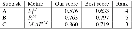
The evaluation metric was different in each sub-task (Nakov et al., 2016). For subsub-task A, it was required to optimize the macro-averaged F1-score
(F1M) calculated over the positive and negative classes. In subtask B, the goal was to achieve a high macro-averaged recall (RM), while subtask C took into account a macro-averaged mean absolute error (M AEM). Table 4 presents the overall performance
of our system.
Subtask Metric Our score Best score Rank
A FM
1 0.576 0.633 14
B RM 0.763 0.797 6
[image:5.612.314.537.339.535.2]C M AEM 0.860 0.719 3 Table 1:Overall performance of the system.
We also performed an analysis of feature impor-tance using one trained Gradient Boosting Trees classifier (GBT). For this classifier the feature im-portance can be easily measured by observing the in-crease of purity while performing splits on a partic-ular feature, following an approach from (Breiman and Friedman, 1984).
In subtasks A and C we used a meta-classifier of many different algorithms, so the results would not accurately reflect the feature importance in the whole system. Hence, we decided to run this exper-iment on the dataset from subtask B only.
Table 2 presents 15 features with the highest
rel-ative importance in our classifier. The most im-portant feature was the mean of word sentiments in a tweet according to the NRC Hashtag Lexicon (the maximum word sentiment on this lexicon is also pretty high in the ranking). Other lexicon fea-tures, based on the Opinion Lexicon and SentiWord-Net, also achieved high relative importance. Note that many features with high importance come from Brown clustering and k-grams.
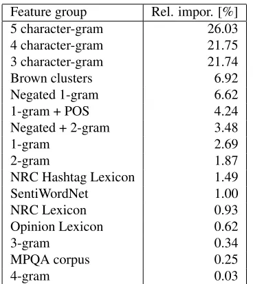
In Table 3, we present results of feature impor-tance aggregated in groups. The most important fea-tures are those created from character k-grams and their total relative importance is almost 70%. The contribution of features created from Brown cluster-ing, negated n-grams and from n-grams with part-of-speech tags is also very significant. The importance of the rest of the features sums up to only 10%. The poor results of lexicon-based features can be justi-fied by the fact that the number of features in these groups is very small (from 2 to 8 features).
Feature name Rel. impor. [%] NRC Hashtag Lexicon: mean 0.79 Brown cluster: 01110110 0.73 SentiWordNet: sum of negative 0.63 5 k-gram: “d &am” 0.55 Brown cluster: 1110011001111 0.49 NRC Hashtag Lexicon: max 0.48 Opinion Lexicon: negative 0.47 Brown cluster: 111101011101 0.42
3 k-gram “ok ” 0.41
4 k-gram “ nor” 0.40
Brown cluster: 0100100 0.38
3 k-gram “ NY” 0.35
2 n-gram: not against 0.35 Brown cluster: 111101111100100 0.34 5 k-gram “ Anth” 0.34
Table 2:Relative feature importances (%) of top 15 features.
For Random Forests and SVM we used feature selection according to the F-statistics. We analyzed how features selected by this approach relate to im-portances estimated by GBT.
[image:5.612.74.300.456.507.2]Feature group Rel. impor. [%] 5 character-gram 26.03 4 character-gram 21.75 3 character-gram 21.74 Brown clusters 6.92 Negated 1-gram 6.62 1-gram + POS 4.24 Negated + 2-gram 3.48
1-gram 2.69
2-gram 1.87
NRC Hashtag Lexicon 1.49 SentiWordNet 1.00 NRC Lexicon 0.93 Opinion Lexicon 0.62
3-gram 0.34
MPQA corpus 0.25
[image:6.612.95.279.55.261.2]4-gram 0.03
Table 3:Relative feature importances (%) for features groups.
only one feature from Brown clustering. How-ever, once again simple n-grams were used very rarely (2% of all selected features). This result, to-gether with earlier observations from importances estimated by GBT, seem to show that features ated from character-grams are superior to those cre-ated by word-grams. It is also worth mentioning that the entire GBT model used only 3579 features, which is an indicator of its feature selection abilities.
5 Conclusions and Future Work
Our system achieved relatively good performance in SemEval-2016 Task 4: Sentiment Analysis in Twit-ter. Among 34 participants of subtask A we reached rank 14, we took 6th place among 19 competitors in
subtask B, and won 3rdplace in subtask C where 11
teams competed. The analysis of features used by our system shows that character-grams seem to per-form better than word n-grams for Twitter’s short-text messages. Furthermore, results obtained by Gradient Boosting Trees in our system confirmed good feature filtering capabilities of this algorithm.
One possible way to further improve our system could be to transfer features selected by GBT to other classifiers (e.g. SVM). Another possible line of the future research is the development of new features based on character-grams, such as negated character-grams or character-gram lexicons.
Acknowledgments
This research was partially funded by the Polish National Science Center under Grant No. DEC-2013/11/B/ST6/00963.
References
Stefano Baccianella, Andrea Esuli, and Fabrizio Sebas-tiani. 2010. Sentiwordnet 3.0: An enhanced lexical resource for sentiment analysis and opinion mining. In
Proceedings of the International Conference on Lan-guage Resources and Evaluation.
Jerzy Błaszczy´nski and Jerzy Stefanowski. 2015. Neigh-bourhood sampling in bagging for imbalanced data.
Neurocomputing, 150, Part B:529–542.
Leo Breiman and Jerome H. Friedman. 1984. Classi-fication and regression trees. Chapman & Hall, New York.
Leo Breiman. 2001. Random forests.Machine learning, 45(1):5–32.
Peter F. Brown, Vincent J. Della Pietra, Peter V. de Souza, Jennifer C. Lai, and Robert L. Mercer. 1992. Class-based n-gram models of natural language. Computa-tional Linguistics, 18(4):467–479.
Corinna Cortes and Vladimir Vapnik. 1995. Support vector machine. Machine learning, 20(3):273–297. Eibe Frank and Mark Hall. 2001. A simple approach to
ordinal classification. InProceedings of the 12th Eu-ropean Conference on Machine Learning, pages 145– 156.
Jerome H Friedman. 2001. Greedy function approxima-tion: a gradient boosting machine.Annals of statistics, pages 1189–1232.
Haibo He and Edwardo A Garcia. 2009. Learning from imbalanced data. Knowledge and Data Engineering, IEEE Transactions on, 21(9):1263–1284.
Shohei Hido, Hisashi Kashima, and Yutaka Takahashi. 2009. Roughly balanced bagging for imbalanced data.
Statistical Analysis and Data Mining, 2(5-6):412–426. Minqing Hu and Bing Liu. 2004. Mining and summa-rizing customer reviews. InProceedings of the Tenth ACM SIGKDD International Conference on Knowl-edge Discovery and Data Mining, pages 168–177. Thorsten Joachims. 1999. Transductive inference
for text classification using support vector machines. In International Conference on Machine Learning (ICML), pages 200–209.
Georg Krempl, Indr˙e ˇZliobait˙e, Dariusz Brzezinski, Eyke H¨ullermeier, Mark Last, Vincent Lemaire, Tino Noack, Ammar Shaker, Sonja Sievi, Myra Spiliopoulou, and Jerzy Stefanowski. 2014. Open challenges for data stream mining research. SIGKDD Explorations, 16(1):1–10.
Mateusz Lango and Jerzy Stefanowski. 2015. Applica-bility of roughly balanced bagging for complex imbal-anced data. In Proceedings of the 4th Workshop on New Frontiers in Mining Complex Patterns (NFMCP 2015), pages 62–73.
Bing Liu. 2012. Sentiment Analysis and Opinion Min-ing. Synthesis digital library of engineering and com-puter science. Morgan & Claypool.
Michael Mathioudakis and Nick Koudas. 2010. Twitter-monitor: Trend detection over the twitter stream. In
Proceedings of the 2010 ACM SIGMOD International Conference on Management of Data, pages 1155– 1158.
Saif Mohammad and Peter D. Turney. 2013. Crowd-sourcing a word-emotion association lexicon. Compu-tational Intelligence, 29(3):436–465.
Preslav Nakov, Alan Ritter, Sara Rosenthal, Veselin Stoy-anov, and Fabrizio Sebastiani. 2016. SemEval-2016 task 4: Sentiment analysis in Twitter. InProceedings of the 10th International Workshop on Semantic Eval-uation.
Olutobi Owoputi, Brendan O’Connor, Chris Dyer, Kevin Gimpel, Nathan Schneider, and Noah A. Smith. 2013. Improved part-of-speech tagging for online conver-sational text with word clusters. In Proceedings of Human Language Technologies: Conference of the North American Chapter of the Association of Com-putational Linguistics, pages 380–390.
F. Pedregosa, G. Varoquaux, A. Gramfort, V. Michel, B. Thirion, O. Grisel, M. Blondel, P. Prettenhofer, R. Weiss, V. Dubourg, J. Vanderplas, A. Passos, D. Cournapeau, M. Brucher, M. Perrot, and E. Duches-nay. 2011. Scikit-learn: Machine learning in Python.
Journal of Machine Learning Research, 12:2825– 2830.
Robert Remus. 2013. Modeling and representing nega-tion in data-driven machine learning-based sentiment analysis. In Proceedings of the First International Workshop on Emotion and Sentiment in Social and Ex-pressive Media: approaches and perspectives from AI (ESSEM 2013), pages 22–33.
Steffen Rendle. 2010. Factorization machines. In Pro-ceedings of the 10th International Conference on Data Mining (ICDM), pages 995–1000.
Abeed Sarker, Azadeh Nikfarjam, Davy Weissenbacher, and Graciela Gonzalez. 2015. Diegolab: An approach for message-level sentiment classification in twitter. In
Proceedings of the 9th International Workshop on Se-mantic Evaluation, pages 510–514.