Analysis of three close eclipsing binary systems: BP Velorum, V392 Carinae and V752 Centauri

(1)

Analysis of three close

eclipsing binary systems:

BP Velorum, V392 Carinae and

V752 Centauri

A thesis submitted in partial fulfilment

of the requirements for the degree of

Master of Science

Hana Josephine Schumacher

2008

(2)

(3)

Abstract

This thesis reports photometric and spectroscopic studies of three close binary systems; BP Velorum, V392 Carinae and V752 Centauri.

BP Velorum, a W UMa-type binary, was observed photometrically in February 2007. The light curves in four filters were fitted simultaneously with a model generated in the eclipsing binary modeling software package PHOEBE. The best model was one with a cool star spot on the secondary larger component. The light curves showed additional cycle-to-cycle variations near the times of maximum light which may indicate the presence of star spots that vary in strength and/or location on a time scale comparable with the orbital period, (P = 0d_._{265). The system was confirmed to belong to the W-type subgroup of W}

UMa binaries for which the deeper primary minimum is due to an occultation.

V392 Carinae, a detached binary with an orbital period of 3d_._{147, was observed}

pho-tometrically by Michael Snowden in 1997. These observations were reduced and com-bined with the published light curve from Debernardi and North (2001). High resolution spectroscopic images were taken using the University of Canterbury’s HERCULES spec-trograph. The radial velocities measured from these observations were combined with velocities from Debernardi and North (2001). The radial velocity and light curves were fit simultaneously, confirming that V392 Car is a detached system of two main sequence A stars with a mass-ratio of 0.95. The derived systematic velocity is consistent with V392 Car being a member of the open cluster NGC 2516.

The W UMa-type binary V752 Centauri was observed photometrically and spectro-scopically during 2007. The high resolution spectra displayed weak sharp lined features superimposed over the strong broad lined spectrum expected from the 0d_._{370 contact}

bi-nary. Fourier methods were used to separate the broad and sharp spectral features and radial velocities for each were measured by cross-correlation. A fit to the photometry and radial velocities for the contact binary implied a system of two late F stars with a mass-ratio of 3.38 in an over-contact configuration. The derived systematic velocity (₋13.8kms−1_{), has changed significantly from the 1972 value (29}_.₂_kms−1_{). The third}

(sharp lined) component’s radial velocities were measured and found to have a period of 5d_._{147, semi-amplitude of 43}_.₄_kms−1 _{and systematic velocity of}

−7.3kms−1_{. The likely}

(4)

(5)

List of Figures

1.1 The orbital plane of the objects as seen from the Earth. . . 2

1.2 A schematic diagram of the Lagrangian points in the Roche model. . . 4

1.3 Configurations of close binary stars given by the Roche Model. . . 6

4.1 Goodness of fit parameter figure taken from Lapasset et al. (1996). . . 21

4.2 BP Vel (O-C) residuals. . . 23

4.3 Goodness of fit parameter determined using models produced by PHOEBE. 24 4.4 The unspotted WD model in BV RI filters. . . 25

4.5 The spotted WD model in BV RI filters. . . 26

4.6 3-D plots of the surface of BP Velorum (with spot). . . 26

4.7 The light curves of BP Vel in the Visual filter. . . 29

4.8 The light curves of BP Vel in the Red filter. . . 29

5.1 The light curve of V392 Car in Stromgren B filter. . . 33

5.2 The light curve of V392 car in Stromgren Y filter. . . 33

5.3 The V-light curve in GENEVA filter of V392 Car. . . 34

5.4 3-D plots of the surface of V392 Car. . . 34

5.5 The combined spectrum of V392 Car. . . 35

5.6 The strong Hβ absorption line from fig 5.5. . . 36

5.7 The cross-correlation function for V392 Car coming into an eclipse. . . 37

5.8 The cross-correlation function of V392 Car near a time of maximum sepa-ration. . . 38

5.9 The Radial Velocity curves from both components of V392 Car including the measurements from Debernardi and North (2001). . . 38

(9)

5.10 The Radial Velocity curves from both components of V392 Car fitted with

the model generated in PHOEBE. . . 40

6.1 The unspotted WD model in BV RI filters. . . 47

6.2 The spotted WD model in BV RI filters. . . 48

6.3 3-D plots of the surface of V752 Cen (with spot). . . 48

6.4 Spectrum of V752 Cen near a time of eclipse. . . 51

6.5 A CCF profile of V752 Cen: the contact binary near a time of eclipse. . . . 52

6.6 A CCF profile of V752 Cen: the contact binary near a time of maximum separation. . . 52

6.7 The sine fit using least squares optimization for V752 Cen. . . 53

6.8 PHOEBE’s model radial velocity curves with the measured velocities from V752 Cen. . . 56

6.9 An example of the CCF of the third component of V752 Cen. . . 58

6.10 The sine fit using least squares optimization for the third component’s total velocities in MATLAB. . . 59

6.11 Schematic diagrams showing the possible geometric configurations of the complete V752 system. . . 60

6.12 Spectrum of V752 Cen near a time of maximum light from the contact binary. 62

(10)

List of Tables

1.1 The details of the three stars analysed in this thesis.. . . 9

2.1 The resolution of HERCULES fibre positions . . . 11

2.2 The dates of the observing runs completed for this research. . . 12

4.1 Photometric Solutions for BP Velorum from Lapasset et al. (1996). . . 22

4.2 Star spot parameters from Lapasset et al. (1996). . . 22

4.3 Star spot parameters determined with PHOEBE. . . 27

4.4 Photometric Solution for BP Velorum determined from our model gener-ated using PHOEBE. . . 28

5.1 The orbital elements of V392 Car. . . 39

5.2 The absolute parameters of V392 Car. . . 40

5.3 Solution of V392 Car determined from PHOEBE. . . 41

5.4 The physical parameters of V392 Car determined by Debernardi and North (2001) . . . 42

5.5 The orbital parameters of V392 Car taken from Debernardi and North (2001). 43 6.1 The derived parameters of V752 Cen taken from Barone et al. (1993). . . . 45

6.2 The orbital elements of V752 Cen . . . 54

6.3 Star spot parameters for V752 Cen. . . 55

6.4 The solution to the spotted and unspotted models from PHOEBE.. . . 57

B.1 The photometric measurements of BP Velorum. . . 86

B.2 The photometric measurements of V752 Centauri. . . 101

B.3 The 1997 photometric measurements of V392 Carinae. . . 142

(11)

C.1 Heliocentric Julian Date, radial velocities of component one and two of V392 Car. . . 151

C.2 Heliocentric Julian Date, radial velocities for the contact binary V752 Cen. 152

C.3 The Heliocentric Julian Date and Radial Velocity measurements for the third component of V752 Cen. . . 154

(12)

(13)

Chapter 1 Introduction

1.1 Binary Systems of Stars:

Historical overview

William Herschel first coined the phrase ‘binary star’ in 1802, to name ‘a real double star - the union of two stars that are formed together in one system, by the laws of attraction’ (Kopal, 1959). The term ‘double star’ had long been used to describe stars in close pairs. The Greek astronomer Ptolemy used it in his Almagest circa 150 A.D.(Ptolemaeus, 1952). However, not all double stars are gravitationally bound and these are therefore, not binary stars. The visual binary systems that Herschel and others observed marked the beginning of a long era of discovery regarding binary systems.

John Goodricke initiated the field of interacting binary stars with the publication of his paper in the Philosophical Transactions of the Royal Society, London, in 1783 (Sahade and Wood, 1978). In this paper he described his independent discovery and observations of the variations in brightness of Algol. The brightness variations of Algol actually had been detected over a century before by Montenari and Miraldi. There is evidence in the writings of ancient Chinese that these variations were known long before. Goodricke himself determined that the variations were periodic and deduced the period.

From the time Goodricke published this paper until the early twentieth century, the approach to observing eclipsing binaries followed the same patterns as for other variable stars. At the start of the twentieth century the observation techniques available were photography, spectroscopy and photoelectric photometry. Throughout the twentieth cen-tury, as the technology of observations improved and fainter objects became observable, the vast occurrence of binary systems became apparent. Recent estimates state that over

(14)

2 CHAPTER 1. INTRODUCTION

80% of all stars may be members of binary systems (Smith, 1995).

The analysis of binary systems can result in the determination of important properties of stars. The fundamental property of mass can be determined without external models from the gravitational effect of some binary systems. Stellar mass is the most intrinsically important property of stars. The knowledge of the initial mass and chemical composi-tion of an isolated star can provide informacomposi-tion related to its structure and subsequent evolution (Ramm, 2004).

1.2 Eclipsing Binary Stars

Binary star systems contain two stars gravitationally bound orbiting about their common center of mass. Eclipsing binary systems, EBs, are systems where the orbital plane lies close to, if not aligned with, the plane of the observer, that is the inclination of the orbit is close to 90◦

(see Figure 1.1). The alignment of the orbital plane with the plane

Figure 1.1: The orbital plane of the objects as seen from the Earth.

of the Earth means the stars eclipse each other periodically. The angular separation of the components as seen from the Earth is not great enough for the components to be resolved individually. The discovery and detection of eclipsing binary systems comes from measuring the variation of the intensity of light through photometry. The observed light intensity varies as the stars move through their orbits. The light curves clearly show the effects of movement of the components of the system.

(15)

1.3. CLASSIFICATION OF CLOSE BINARY SYSTEMS: THE ROCHE MODEL 3

light curve data double-lined spectroscopic binaries can be used to determine the indi-vidual masses of the stars, their radii, the ratio of their fluxes and hence the ratio of their effective temperatures. Equipped with the photometric and spectroscopic orbital solutions of an eclipsing binary, a star’s radius can be estimated to a high precision, indicating the star’s evolutionary state (Ramm, 2004).

The components in close binary systems have undergone gravitational stresses which have resulted in circular and synchronous orbits. Stellar rotation through the tidal bulge raised by the companion’s gravitational pull, causes the star to pulsate. Orbital and rotational energy are dissipated until the system reaches the state of minimum energy for its constant angular momentum which inspires synchronous rotation and circular orbits (Carroll and D.A. Ostlie, 1996).

In the cases where the binary system’s components are well detached, the separate components undergo stellar evolution as one would expect from a single star. The gravi-tational effect from the companion star does not appreciably alter the shape of the star. However, in the cases where the separation of the components is very little, there is mass exchange between the components, and their evolutionary progress departs that of a single star corresponding to the same position on the main sequence of an H-R diagram (Sahade and Wood, 1978). These are known asinteracting orcontact binaries.

Contact binary systems are defined to be systems ‘which have both components sur-rounded by a common envelope lying between the inner and outer Lagrangian zero-velocity equipotential surfaces’ (Mochnacki, 1981). Systems which are of spectral type F0 and later are usually referred to as W Ursae Majoris stars (W UMa).

1.3 Classification of Close Binary Systems: The Roche

Model

(16)

[image:16.595.136.448.210.474.2]

of the star. In this region the equipotential surfaces are nearly spheres so the attraction on a point near the exterior of the star is approximately the same as for the Roche model (Sahade and Wood, 1978). The closer a stellar surface is to an equipotential surface the more it takes the shape of that surface.

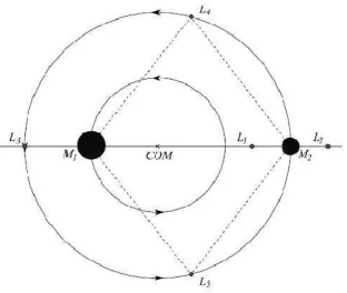
Figure 1.2: A schematic diagram of the Lagrangian points in the Roche model from

PHOEBE Scientific Reference (Prˇsa, 2006).

The surfaces are also known as the zero-velocity or Roche surfaces, with the shape of these surfaces depending on the Lagrangian points. Lagrange’s work established points in the rotating field of the two massive bodies where the third body has zero velocity; these are known as the Lagrangian points. The first of these points is located on the axis between the two massive bodies. This is often called the inner Lagrangian point L1, and

it is an unstable equilibrium point. The Roche surfaces that meet at this point are called the Roche limits. They encompass the Roche lobes, a critical feature in the classification of close binary systems. There are two more Lagrangian points along this axis; L2 is

located beyond the outer surface of the lesser mass, L3 is similarly located outside the

outer surface of the larger mass. There are two other Lagrangian points corresponding to potential maxima, L4 and L5. They form equilateral triangles with the two masses. The

(17)

1.3. CLASSIFICATION OF CLOSE BINARY SYSTEMS: THE ROCHE MODEL 5

depending on whether their respective Roche lobes are filled or not. L2 and L3 provide a

route to which the system as a whole can lose mass. The filling of the Roche lobes may be determined through the fill-out factor which can be derived from the normalised total potential ψ(r, q) at point r (Mochnacki and Doughty, 1972):

ψ(r, q) = 2 1 +q

1

rn +

2q

1 +q

1

rl +p

2

=C, (1.1)

where q is the mass ratio of the lighter mass ml, with the heavier mass mh. The distance fromrto the center of the lighter and heavier components,rl andrh respectively,

p is the perpendicular distance from the axis of rotation. Equipotential surfaces are classified by the constantC ofψ(r, q) (Mochnacki and Doughty, 1972). The fill-out ratio

F, is used to determine the degree to which the equipotential surface of the photosphere fills its corresponding Roche lobe. Cp is the photospheric potential,C1(q) is the constant

corresponding to the Roche limit, and C2(q) is the constant for the second Lagrangian

surface L2. For a completely detached binary the fill-out ratio is defined as

F = C1

Cp, (1.2)

where Cp _≥C1(q) and 0< F ≤1. For a contact configuration, the fill-out factor is

F = C1−Cp

C1−C2

+ 1, (1.3)

where C1(q) ≥ Cp ≥ C2(q) and 1 ≤ F ≤ 2. Note for the contact configuration the

entire envelope over both components is specified by a single surface potential value, Cp

(Mochnacki and Doughty, 1972).

The fill-out factor is a convenient way to determine the configuration of the close binary system. Kopal (1959) specifies 3 categories from the Roche model classification scheme with two additional sub-categories;

1. Detached systems: the Roche limit is not exceeded by either component. The components’ shapes are determined by inner Roche surfaces and are nearly spherical.

2. Semi-detached systems: one component exactly fills its Roche limit. There is mass transfer via the inner Lagrangian pointL1.

3. Contact systems: both components fill their Roche lobes.

(18)

by the equipotential that has equatorial material rotating at close to the centrifugal limit.’ (Ramm, 2004).

3b. Over-contact systems: the systems have the components surrounded by a common convective envelope.

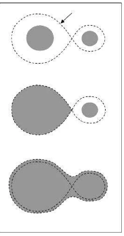
[image:18.595.159.372.268.672.2]

W UMa-type contact binaries fall into the over-contact category. Figure 1.3 illustrates three configurations, the inside dotted line depicts the Roche limit. The top figure is a de-tached binary, the middle figure is a semi-dede-tached configuration, the bottom illustration shows an over-contact configuration.

Figure 1.3: An illustration of the various configurations of close binary stars as given by

(19)

1.4. W UMA-TYPE BINARIES 7

1.4 W UMa-type Binaries

W Ursae Majoris systems are prolific in the contact binary population, they are of spectral type F0 and later. The large population of W UMa-type binaries indicate that they are not all formed as a result of detached binaries evolving into contact and were therefore created as binaries in contact on the zero-age main sequence, ZAMS (Lucy, 1968b). They typically have very short periods (_≤0.5 days), which often makes it possible for complete light curves to be observed in one night. Their light curves show strong characteristics. The light variation is continuous, with the minima nearly equal in depth (Lucy, 1968a).

W UMa-type systems can be further classified into two sub-groups; A-type systems and W-type introduced by Binnendijk (1965). The W-type systems are defined as having the primary minimum resulting from an occultation of the secondary, less massive component; A-type systems have the deeper minimum corresponding to a transit of the secondary in front of the primary, more massive component (Mochnacki, 1981).

Generally A-type systems are of earlier spectral type and more evolved (Mochnacki, 1981). A-type systems generally have lower mass ratios and a higher degree of contact than W-type systems. Light curves of W-type systems often have asymmetries, whereas in light curves from A-type systems asymmetries are more moderate or even absent.

Lucy (1968b) proposed a model with a convective envelope surrounding the two com-ponents that allowed W UMa-type binaries to be created on the ZAMS with different initial radii. The convective envelope model successfully interpreted the characteristics of the distinctive light curve of W UMa-type binaries, while simultaneously explaining the near equal temperatures and luminosities of the components even though they can have highly different masses (Csizmadia and P. Klagyivik, 2004).

Hilditch (2001), explains the general consensus surrounding the formation of W UMa-type contact binaries being that they formed from detached systems of low mass and orbital periods of 1 day or less. Orbital angular momentum is lost from the detached system due to magnetic stellar wind causing the orbit to shrink. The shrinking of the orbit leads to the shrinking of the Roche lobes to the extent where overflow of the Roche lobe occurs by the primary onto the secondary. Eventually contact is made, though this can be tenuous as the system alternates about a state of marginal contact for an uncertain length of time before coalescing into a single star (Vilhu, 1982; Bradstreet and Guinan, 1994).

(20)

envelope theory of Lucy (1968a).

1.5 Motivation for this work

The three targets analysed in this work are displayed in table 1.1. They were selected on a criteria comprising of a few complimentary points. Firstly, the targets’ observability from the telescope facilities at Mt John University Observatory and the time frame under which the thesis was to be conducted. The suitable candidates from the initial sorting were contemplated and decided upon regarding their exposure in literature.

The target BV Velorum has previously been observed photoelectrically with the results published in Lapasset et al. (1996). The faint magnitude of BP Velorum has made it difficult to study spectroscopically. The photometric observations of this target used in this thesis were undertaken during one week using the Optical Craftsman telescope at Mt John University Observatory mounted with the SBIG ST-9 CCD camera. The solution determined by Lapasset et al. (1996) provides a good check on the methods used throughout this thesis. The faintness of the target meant that no spectroscopic observations were made as it was beyond the limits of the HERCULES instrument.

V392 Carinae, also nominated Cox 38, belongs to the open cluster NGC 2516. It was observed photometrically at the European Southern Observatory, La Silla, Chile from January 1978 to January 1991. Spectroscopic observations were performed at the same sight over two nights during February 1991. The orbital elements of V392 Car were calculated by Debernardi and North (2001) who found the system was indeed a member of NGC 2516 and that the stars were of spectral type A2. The phase coverage of the spectroscopic observations is very poor. We were approached by Michael Snowden to make further spectroscopic observations of this star to combine with imaging photometry he had undertaken in 1997.

V752 Centauri has been analysed both photometrically and spectroscopically. Com-plete light curves were observed photoelectrically in 1971 by Sisteró and Castore de Sisteró (1973) and radial velocity curves were measured from spectrograph observations taken in 1972 ( Sisteró and Castore de Sisteró, 1974). Leung (1976) reanalysed the observations taken by Sisteró and Castore de Sisteró using the Wilson and Devinney code. Barone et al. (1993) reanalysed the archival data for V752 Centauri in 1993 with their Wilson-Price code.

(21)

1.5. MOTIVATION FOR THIS WORK 9

Name R.A. (J2000) Dec. (J2000) V max. mag. Period BP Velorum1

08h₁₈m₀₅_.₈s

−45◦ 23′

26′′

12.9 0d_._2649859700

V392 Car1 ₀₇h₅₈m₁₀_.₅s ₋₆₀◦ 51′

57.2′′

9.48 3d_.₁₇₄₉₉₀∗ V752 Cen1 ₁₁h₄₂m₄₈_.₁s ₋₃₅◦

48′ 58′′

9.1 0d_._37022484

Table 1.1: The details of the three stars analysed in this thesis.

1 _{VizieR catalogue information (Viz).}

∗

Period taken from Debernardi and North (2001).

(22)

Chapter 2 Observations

The photometric and spectroscopic observations used in this work were all taken at Mt John University Observatory (MJUO), Lake Tekapo, New Zealand (170◦

27.9′

E, 43◦ 59.2′ S).

2.1 Photometry

The light curves of the three EB’s were obtained from photometric observations conducted with the 0.6m Optical Craftsman telescope.

The photometric observations for BP Velorum and V752 Centauri were taken by the author, using the Optical Craftsman telescope, (O.C.), from February to April 2007. The O.C. is a 0.61m reflector with a cassegrain focus of f/16 equipped with the AAVSO CCD. The CCD camera is a SBIG ST-9e type. It is 512 by 512 pixels, each 20µ m_×20µ min size, corresponding to a 9′

by 9′

field of view of the sky. The gain is 2.4 electrons per A.D.U. The CCD is thermoelectrically cooled to at least 10◦

below ambient temperature. The camera has a filter wheel with four colours; B,V,R and I in the Johnson-Cousins system. It is operated with the CCDSOFT software which can be programmed to capture an image through each of the filters in turn. The Infrared filter was the most sensitive leading to shorter exposure times. The exposure times for each filter were varied from night to night depending on the atmospheric seeing.

Dark, bias, and flat field frames were taken once or twice during each run of obser-vations. The flat field images, in each filter, were obtained using a light mounted to the wall of the telescope building shining onto a white screen.

(23)

2.2. SPECTROSCOPY 11

2.2 Spectroscopy

The High Efficiency and Resolution Canterbury University Echelle Spectrograph, (HER-CULES), on the 1m McLellan telescope was used to observe V752 Centauri and V392 Carinae. BP Velorum, with a visual magnitude of 12.9, is too faint to observe with HERCULES.

The McLellan telescope is a reflecting telescope of diameter one metre. It was used with the configuration of a cassegrain focus of f/13.5, with the HERCULES system fed by an optical fibre with the 100µm diameter.

2.2.1 HERCULES

HERCULES is a fibre-fed echelle spectrograph which has been operational at MJUO since April 2001. The spectrograph consists of a large R2 echelle grating to provide primary dispersion. Cross-dispersion is achieved with a prism which gives higher efficiency at all wavelengths than conventional grating instruments. The whole instrument is situated inside a vacuum tank where the pressure is maintained at 1-5 torr. The tank resides in a thermally isolated and insulated room.

The light collected from the telescope is guided to HERCULES by optical fibre. There are three possible fibres for use as shown in table 2.1, the choice of which is controlled with a dial at the telescope. Fibre 1 is 100µm in diameter and provides a resolving power of 41000. Fibre 2 has a core diameter of 100µm superimposed by a 50µm micro slit and resolving power of 70000. Fibre 3 has a core diameter of 50µm with resolving power of 82000 (Hearnshaw et al., 2002).

Fibre Position Diameter Resolution

1 100µm 41000

2 100µm with 50µm slit 70000

3 50µm 82000

Table 2.1: The resolution of HERCULES fibre positions

(24)

12 CHAPTER 2. OBSERVATIONS

and thus the effect of blending would become important. Generally, an integration time less than 10% of the orbital period can avoid the effect of spectral line blending.

The exposure times for V392 Carinae varied from 1800 seconds to 3600 seconds and had a lower signal to noise. However, due to the longer period of V392 Car, the longer integration time was not comparable to the orbital period. The guiding camera on the telescope has difficulty at fainter magnitudes and 9th _{magnitude appeared to be its limit.}

The readout speed was chosen to be 200kHz, this has a slightly higher readout noise value than that corresponding to a readout speed of 100kHz, however it has a lesser value for the gain at 1.18, which, given the faint magnitude of the targets, was deemed a more important factor.

Each night radial velocity standards were observed and calibration images of white lamp and thorium lamp were taken. There were several spectra of poor quality which were not used in the radial velocity measurements.

Date Target Telescope Instrument Observations

14-19 February 2007 BP Velorum O.C. S BIG ST9 CCD 1250 BVRI photometry

19-26 March 2007 V752 Centauri O.C. S BIG ST9 CCD 3836 BVRI photometry

10-15 April 2007 V752 Centauri O.C. S BIG ST9 CCD 1665 BVRI photometry

12-15 May 2007 V752 Centauri McLellen 1m HERCULES 21

V392 Carinae Spectroscopy 8

23-27 June 2007 V722 Centauri McLellen 1m HERCULES 30

V392 Carinae Spectroscopy 18

25-27 July 2007 V392 Carinae McLellen 1m HERCULES 3 Spectroscopy

(25)

Chapter 3 Reductions and Software

3.1 Photometry

The photometric images were all reduced using the MIRAMETRICS software MIRA AL.

3.1.1 MIRA AL

MIRA AL is a Microsoft Windows based photometric reduction software package. The software is widely used as a tool for differential photometry and uses equation 3.1 for the calculation of magnitudes.

m =K₋2.5 log(f lux) (3.1)

whereK is the photometric zero point and f lux=Gain_∗Counts/Exptime.

3.1.2 Reducing Photometric Images

The calibration frames were combined prior to the reduction of the data images. The bias frames were combined using the Mean method which calculates the arithmetic mean value at each pixel location and creates a master image. The pixels are combined with no weighting or rejection of bad values which is the preferred method for image sets which can be considered to contain well behaved statistical noise. The dark frames were combined by collecting the median values at each pixel location to create an image. This method, called the Median method, is effective for excluding extreme values. The flat field frames for each filter are combined using the Median method and the combined image is then normalised. Calibration of the images was completed following the steps below.

(26)

14 CHAPTER 3. REDUCTIONS AND SOFTWARE

1. The set of bias images were combined using the Median method to create a Master Bias frame.

2. Each dark frame of a certain exposure length, had the Master Bias subtracted and then the bias subtracted darks were combined with the Mean method creating a Master Dark frame.

3. The flats from each filter were Master Bias and Master Dark subtracted. Each filter set was then combined using the Median method. The combined image was normalised creating the Master Flat.

4. Each data image had the Master Bias and the Master Dark (with the same exposure time) subtracted and then divided by the Master Flat. The processed data frame was then ready to be measured.

For all exposure times used for the data images, dark frames were taken. This saved the process of scaling the master dark images.

MIRA’s aperture photometry tool was used to measure the differential magnitudes of the target with respect to three or more comparison stars within the same field. The com-parison stars used were tested for variability by taking measurements of the comcom-parison stars with respect to each other. With the comparison stars such a small distance from the target stars, each are equivalently affected by the atmospheric conditions.

The aperture photometry procedure allows the aperture sizes to be defined; the inner annulus encompasses the star while the outer annulus determines the background sky counts. The target can be calibrated against as many comparison stars as the field allows. In all measurements made for this research at least three comparison stars were used with each field. The more comparison stars used in the differential measurement the less biased the measurements of the target are. The output resulting from the aperture photometry is the relative magnitudes of both the target and the comparisons along with the signal to noise and error measurement. The Julian Dates are calculated in MIRA from the date and universal time given in the Fits header files.

(27)

3.2. REDUCTION OF THE SPECTROSCOPIC IMAGES 15

3.1.3 Heliocentric Correction

The finite velocity of light and the orbital motion of the Earth about the Sun introduces a shift in the dates of stellar measurements. To account for the possible differences in the timings of the observations, the point of reference for the observations is altered to the Sun which by comparison has negligible movement. The correction can be calculated and applied with equations 3.2 and 3.3.

HJD=JD(geo) +HelCorr (3.2)

HelCorr=T R(cosLcosAcosD) +T R(sinL(sinEsinD+ cosEcosDsinA)) (3.3)

T = time for light to travel 1 A.U._≈499s

R = Earth-Sun distance L = Longitude of the Sun A = Star’s right ascension D = Star’s declination

E = obliquity of the ecliptic 23.45◦

The heliocentric corrections were calculated for the photometric data in the EXCEL programme written by Dan Bruton, SFA Observatory.

The heliocentric corrected measurements were then imported into MATLAB where the period was converted into the phase. The corresponding data was converted into an ASCII file which is flexible and can be used in the PHOEBE software.

3.2 Reduction of the Spectroscopic Images

The images acquired with the HERCULES spectrograph were reduced with the Hercules Reduction Software Package (HRSP) (Skuljan, 2007).

(28)

correction is not applied to the spectrum and is later applied using FIGARO’s vachel

command.

The spectra were intended to be reduced with the wavelength calibration in air rather than in vacuum. A new version of HRSP was used for the reduction process and un-beknown at the time, the dispersion solution configuration files within the new version HRSP were switched. This resulted in our spectra having wavelength calibrations in vac-uum. It was later determined, (see equation 3.6), that this systematic error could be removed by applying a correction to the derived radial velocities.

3.3 Preparation of the Spectra

An important step in the cross-correlation preparation is fitting a continuum to the echelle orders. Applying a continuum normalises the spectrum to unity at each continuum point, ensuring the comparison with the template spectrum has been made with the same level of continuum (unity). The continuum fitting process employed in this research is a routine which fits a low order polynomial equation to the raw spectrum, this is repeated to minimise the residuals. For early type stars the absence of strong metallic lines means there is a strong presence of a reliable continuum throughout the spectrum. For later type stars where the metallic lines become stronger there is less continuum to work with. The automated routine was checked with the manual continuum fitting process cfit in FIGARO.

The low signal to noise, and long exposure times of these targets brought in more cosmic rays. The HRSP filtering of cosmic rays did not clean all of the spikes in the spectra. The continuum fitted spectra were run through a filtering procedure to further clean them of spikes.

3.4 Cross-correlation of the Spectra

The Doppler shift is used to measure the radial velocity of a star. This can be done by measuring the horizontal shift of a single line in the spectra with respect to a reference point. The shift can be translated into the Doppler shift and hence the velocity, if the horizontal axis has a logarithmic scale.

∆λ λ0

= v

(29)

3.4. CROSS-CORRELATION OF THE SPECTRA 17

However, the velocity from the Doppler shift determined from just one specific spectral line cannot be expected to be very accurate as different lines are created at different depths of the photosphere hence are subject to different temperatures and velocity gradients (Ramm, 2004).

Measuring the average velocity from a large number of lines provides a more accurate velocity. The technique of cross-correlation uses a convolution between the programme spectrum and a template spectrum. The convolution is made simpler when done in Fourier space. If the spectrum is in a logarithmic scale the velocity can be directly measured. The spectrum of an SB2 binary with its complicated splitting of spectral lines is a worthy candidate for the cross-correlation technique. Cross-correlation with a suitable template spectrum provides a single smoothed profile which can be easily and reliably measured giving the radial velocity.

Thecross-correlation function c(x), CCF, shown in equation 3.5 as the convolution of two functionsf(k) andg(k), takes a value equal to the integral of the product of the two functionsf(k) andg(k₋x). The integral is evaluated for a range of values ofx and c(x) provides a numerical description of how well the functions f(k) and g(k) are matched (Hilditch, 2001).

c(x) =

Z +∞ −∞

f(k)g(k₋x)dk. (3.5)

The CCF may then yield the shift in the program spectrum with respect to the tem-plate spectrum and, with the temtem-plate’s velocity well determined, the relative velocity of the program spectrum can be measured.

The cross-correlations performed in this thesis make use of the fast-Fourier-transform algorithm (FFT), and IFFT functions of MATLAB. The templates used are synthetic templates generated with temperatures corresponding to the spectral types of targets. The FFT requires a spectrum as free as possible of sharp discontinuities which exist at the ends of each echelle order. To remedy this, ten percent from the ends of the spectra are smoothed with a cosine bell function, causing the ends to gradually taper to zero (Brault and White, 1971).

The FFT’s were performed in MATLAB using a script written by Dr. Michael Albrow (see Appendix A). For the target V752 Cen, with the unusual behaviour of its spectrum (see Chapter 6), the cross-correlation is performed with two templates. The program spectrum is first split into two by determining and applying high-pass frequency and low-pass frequency filters.

(30)

thegauss command from the FIGARO software package. The error estimate on all radial velocities measured in this thesis is adopted as 2kms−1 _{which is approximately 1% of the}

average width of the CCF peaks.

As discussed in Section 3.2, the spectra were reduced with vacuum rather than air wavelengths. Images calibrated with air wavelengths is the international standard. Equa-tion 3.6 can make the conversion from vacuum to air1_;

λAIR= λV AC

1.0 + 2.7352_×10−4₊131.4182

λ2

V AC +

2.7625×108

λ4

V AC

. (3.6)

The vacuum to air conversion was calculated for the radial velocities using a linearised version of equation 3.6 that neglected the final two terms in the denominator, with equa-tion 3.4. The difference in ∆V using the full equation 3.6 or using the modified equation was well within the measurement uncertainty of the radial velocities, so the constant correction of ₋82.0338kms−1 _{to the final velocities was used.}

3.5 The Spectroscopic Orbital Solution

For spectroscopic binaries where both components’ radial velocities are measurable, it is possible to determine the spectroscopic orbital solution.

For circular orbits, eccentricity e = 0, the radial velocity curves may be fitted with equation 3.7;

Vn =γn+Knsinθ, (3.7)

wheren= 1 or 2 andγ is the systematic velocity, K is the semi-amplitude of the velocity curve and θ is the phase angle.

The mass-ratio q can be determined from the ratio of the semi-amplitudes q = K2

K1.

The projected semi-major axis may also be determined by

ansini= (9.1920_×10−5

)KnP√1₋e2_,₍_AU₎_. _(3.8)

If the inclination is known, the components individual masses may be determined from equation 3.9;

M1,2 = (1.0361×10

−7

)_×P K2,1(K1,2 +K2,1)2

√

1₋e2

sini

3

,(M⊙). (3.9)

(31)

3.6. PHYSICS OF ECLIPSING BINARIES 19

3.6 PHysics Of Eclipsing BinariEs

The PHysics Of Eclipsing BinariEs software, PHOEBE, was released under the GNU public license. It is a modeling software for eclipsing binaries which uses the Wilson-Devinney code. The Wilson-Wilson-Devinney code, WD code, computes a synthetic model of an eclipsing binary which is based on the Roche model. The inverse problem is solved using differential corrections. At PHOEBE’s core, the modeling engine is running on WD-2003, the next layer consists of the incorporations of all scientific, numerical and technical extensions. At the outermost layer there is an user interface, serving as a bridge between the user and the model (Prˇsa, 2006).

PHOEBE uses differential corrections, DC, to derive the χ2

minimization. The dif-ferential corrections method was first proposed by Euler (1755). It is based on replacing partial derivatives with finite differences and is one of the most straight forward numerical methods to determine the best fit (Prˇsa, 2006).

PHOEBE offers the user five options for the system’s configuration: A general system with no constraints, a detached system, semi-detached system, double-contact, and two over-contact configurations: W UMa-type and one where the components are not in ther-mal contact. The model type selected adds constraints depending on the configuration.

The underlying WD code can be driven through either the scripter or the PHOEBE Differential Corrections Minimization window. After each iteration, the DC Minimiza-tion window displays the parameter name, the original value, the correcMinimiza-tion amount, the corrected value and the standard deviation of the corrected value.

(32)

Chapter 4 BP Velorum

BP Velorum was discovered to be variable by de Koort in 1941 (Lapasset and Gomez, 1988), who obtained a photoelectric light curve and declared BP Vel to be a W UMa-type eclipsing binary system. Lapasset and Gomez (1988) observed BP Vel photoelectrically at Complejo Astronomico El Leoncito in Argentina with the 215cm telescope using the Vatican Observatory polarimeter as a photometer. From a total of 930 observations twelve times of minima were calculated. They deduced the depth of the primary and secondary minima to be 0.8 and 0.6 magnitudes.

Lapasset and Gómez revisited BP Vel along with Fariñas in 1996 in their collective work on three W UMa-type systems (Lapasset et al., 1996). Using the observations from Lapasset and Gómez (1988), Lapasset et al. (1996) analysed the light curve of BP Vel, which they found to belong to the W subclass of W Uma-type systems with asymmetries in the light curves modeled with cool spots on the more massive secondary component.

4.1 Previous Model

Using the Wilson-Devinney routine to model the light curves, Lapasset et al. (1996) derived the parameters listed in table 4.1. They used the WD code with a range of 18 fixed mass ratio values between 0.3 and 3.0, to obtain the best initial estimate ofq. Their models for each given q had the following adjustable parameters: the inclination (i), the potential (Ω1 = Ω2), the polar temperature of the secondary component (T2), and the

relative monochromatic luminosities (L1V, L1B). They held fixed the polar temperature of

the primary component (T1), the gravity-darkening coefficients (g1 =g2), the bolometric

albedos (A1 = A2) and the limb-darkening coefficients (X1V = X2V, X1B = X2B) along

with the mass ratio (q).

(33)

4.2. PREPARATION OF THE LIGHT CURVES 21

The mass ratio which determined the solution with the best value of the sum of the squared weighted residuals was found to be q = 1.9. The sum of the squared weighted residuals, Σ(wr2_{), is termed the goodness-of-fit parameter. Figure 4.1 is the plot made}

[image:33.595.174.456.208.468.2]

by Lapasset et al. (1996). They adopted the solution determined when q = 1.900 as the unspotted solution for BP Vel.

Figure 4.1: Goodness of fit parameter,[S(q) = P

ωr2 ₌ P

ω(Iobs−Ith)2] vs. the mass ratioq=m2/m1. Figure taken from Lapasset et al. (1996).

Since the theoretical light curve did not satisfactorily fit the observed points and there were systematic ambiguities in the residuals, a star spot with the parameters in table 4.1 was added to the solution. The spotted solution was found to yield a better fit between the theoretical and the observed light curves.

4.2 Preparation of the Light Curves

(34)

22 CHAPTER 4. BP VELORUM

Unspotted Solution Spotted Solution

q 1.900∗

1.8778_±0.0004

i 81.60_±0.24◦

82.08_±0.13◦

T1 5000◦Ka 5000◦Ka

T2 4705±7◦K 4717±4◦K

Ω1 = Ω2 5.047±0.006 4.998±0.007

F = Ωin−Ω

Ωin−Ωout 10.05±0.6% 14.0±0.7%

g1 =g2 0.32a 0.32a

A1 =A2 0.50a 0.50a

X1V =X2V 0.712a 0.712a

X1B =X2B 0.866a 0.866a

L1

L1+L2(V) 0.440 0.439

L1

L1+L2(B) 0.449 0.448

r1(pole) 0.309 0.312

r1(side) 0.324 0.327

r1(back) 0.360 0.364

r2(pole) 0.415 0.416

r2(side) 0.442 0.443

r2(back) 0.472 0.474

Table 4.1: Photometric Solutions for BP Velorum from Lapasset et al. (1996).

Note: a_{N ot altered.}

Location Secondary Colatitude 90◦

(adopted) Longitude 99.8_±0.1◦ Spot Radius 14.7_±3.0◦

Tspot

Tstar 0.76±0.09

Table 4.2: Star spot parameters from Lapasset et al. (1996).

from equation 4.1, where Pest was the period taken from Viz, (Pest = 0d_._{26498597), and} E is the epoch.

C =HJD0+PestE. (4.1)

(35)

4.3. MODELING WITH PHOEBE 23

−10 −5 0 5 10 15

−4 −3 −2 −1 0 1 2 3 4x 10

−3

Epoch

O−C (days)

Figure 4.2: BP Vel (O-C) residuals of minimun light showing the ten epochs in the four

filters.

P = Pest +b where b is the slope in the line. The new period was found to be P = 0d_.₂₆₅₀₃₄

±0d_._{000048. From a linear least-squares fit of the ten times of observed minimum}

in our data, the ephemeris was found to be

HJD0 = 2454147.934346(±0.00002) + 0.265034(±0.00005)

The reduced data was phased with the new period and then modeled with PHOEBE.

4.3 Modeling with PHOEBE

The PHOEBE configuration option of an over-contact system of the W UMa-type was attempted for the first fit. The results were not satisfactory however, the difference in the minimum depths was not sufficiently matched and the temperature of the primary diverged rather dramatically.

An over-contact system without thermal contact was found to be the best configuration option for BP Vel. This option, while complying with the contact configuration condition, that the potentials are equal Ω1 = Ω2, allowed the temperatures of the primary and

the secondary to differ. The different temperatures drove the model to match BP Vel’s observed minimum inequality. The primary minimum is around 0.15 mag deeper than the secondary eclipse in all filters.

(36)

method would be employed for further light curve analysis. From Figure 4.1, a range of mass ratio values to test was decided upon. The values of q that we used, ranged from 1.2_≤q _≤2.4.

1.2 1.4 1.6 1.8 2 2.2 2.4 2.6

1.46 1.48 1.5 1.52 1.54 1.56

1.58x 10

−5

mass ratio (q)

[image:36.595.154.406.171.374.2]

S

Figure 4.3: Goodness of fit parameter,[S(q) =P

ωr2 ₌P

ω(O₋C)2_]_{vs. the mass ratio}

q=m2/m1, determined using models produced by PHOEBE for BP Vel. The circled value

is theq used as a start point in the unspotted and spotted models.

The WD code was implemented on fixed values of q within this range, leaving the relative monochromatic luminosities (L1(B, V, R, I)), the primary and secondary

tem-peratures (T1, T2), the potential (Ω1 = Ω2), the inclination (i) and the limb-darkening

coefficients (X1(BV RI) and X2(BV RI)) free to converge. The gravity-darkening

coeffi-cient and the bolometric albedo were fixed at g1 = g2 = 0.32 and A = 0.5. The values

for q and A follow the convective envelope model for contact binaries taken from Lucy (1968a) and Ruci´nski (1969). The spectral type of BP Vel is KI so the initial value chosen for the temperatures of both components was 5000K (Lapasset et al., 1996). The limb-darkening coefficients were calculated using a square root limb-limb-darkening law after each set of iterations.

The fit of the model was judged on the sum of the squared weighted residuals (S = Σ(wr2_{) = Σ(}_O

−C)2_{). The values of} _S _{were plotted against} _q _{in Figure 4.3. The} _q _that

gives the best model isq = 2.1 compared with q= 1.9 found by Lapasset et al. (1996).

4.3.1 Unspotted Model

(37)

4.3. MODELING WITH PHOEBE 25 0.04 0.05 0.06 0.07 0.08 0.09 0.1 0.11

-0.6 -0.4 -0.2 0 0.2 0.4 0.6

Total Flux

Phase

(a) Blue filter

0.06 0.07 0.08 0.09 0.1 0.11 0.12 0.13 0.14

-0.6 -0.4 -0.2 0 0.2 0.4 0.6

Total Flux

Phase

(b) Visual filter

0.06 0.07 0.08 0.09 0.1 0.11 0.12 0.13 0.14 0.15

-0.6 -0.4 -0.2 0 0.2 0.4 0.6

Total Flux

Phase

(c) Red filter

0.08 0.09 0.1 0.11 0.12 0.13 0.14 0.15 0.16

-0.6 -0.4 -0.2 0 0.2 0.4 0.6

Total Flux

Phase

(d) Infrared filter

Figure 4.4: The unspotted WD model inBV RI filters.

The unspotted model was generated leaving the parameters described in the preced-ing section and the mass-ratio free. The goodness of fit for the unspotted model was

S = 1.41_×10−05

. The observed light curves show unevenness at their maxima. This is more pronounced in the visual and red filters which rules out systematic errors from the instruments. If it were a case of a systematic error, one would expect it to be continued through the other filters and that there would be just as much scatter at minimum light. Lapasset et al. (1996) discovered a model with a star spot added to the secondary com-ponent produced the best fit. The placing of the star spot on the secondary comcom-ponent at the equator was repeated for this analysis.

4.3.2 Spotted Model

As shown in Figure 4.4 it is obvious there is some effect toying with the light curve near phase ₋0.25 in the Visual and Red filters. A star spot was placed on the secondary component at a colatitude of 90◦

(38)

26 CHAPTER 4. BP VELORUM 0.04 0.05 0.06 0.07 0.08 0.09 0.1 0.11

-0.6 -0.4 -0.2 0 0.2 0.4 0.6

Total Flux

Phase

(a) Blue filter

0.06 0.07 0.08 0.09 0.1 0.11 0.12 0.13 0.14

-0.6 -0.4 -0.2 0 0.2 0.4 0.6

Total Flux

Phase

(b) Visual filter

0.06 0.07 0.08 0.09 0.1 0.11 0.12 0.13 0.14 0.15

-0.6 -0.4 -0.2 0 0.2 0.4 0.6

Total Flux

Phase

(c) Red filter

0.08 0.09 0.1 0.11 0.12 0.13 0.14 0.15 0.16

-0.6 -0.4 -0.2 0 0.2 0.4 0.6

Total Flux

Phase

(d) Infrared filter

Figure 4.5: The spotted WD model in BV RI filters.

(a) phase = -0.25 (b) phase = 0

(c) phase = 0.25 (d) phase = 0.5

(39)

4.4. SOLUTION 27

again to account for the star spot. The resulting model is plotted with the observed light curve in Figure 4.5. The spotted solution has a goodness of fitS = 1.35_×10−5 _compared

with S= 1.41_×10−5 _{for the unspotted solution.}

Location Secondary Colatitude 90◦

(adopted) Longitude 140.9_±0.04◦ Spot Radius 8.0_±1.7◦

Tspot

Tstar 0.79

Table 4.3: Star spot parameters determined with PHOEBE.

The light curves from each night of observation were investigated for evidence of fluctuation in intensity at the times of maximum light. The reason for this investigation is the idea that variability in star spots’ location and/or strength would show up in the light curves. The times of maximum light may show variations from night to night as the spots travelled across the hemisphere facing us. Figures 4.7 and 4.8 show theV and

R filters’ observations of BP Velorum from five nights in February 2007. The maxima leading into the primary eclipse (phase=1.0 in Figures 4.7 and 4.8), show a dip in the intensity of light moving from the left to the right over three nights. These variations in the light curves are not thought to be due to random scatter since at the times where the least light is coming from the system, the light curves do not show scatter.

4.4 Solution

The photometric solution for BP Vel determined in this thesis produced slightly different values for the parameters than the solution Lapasset et al. (1996) found, the values for the parameters is shown in table 4.4. Figure 4.6 displays the surface of the spotted model of BP Vel at different phases.

(40)

Unspotted Solution Spotted Solution

q 2.1344_±0.0108 2.198_±0.0045

i 83.81_±0.25◦

83.37_±0.23◦

T1 5189±9.6K 5184±9.3K

T2 4846±8.4K 4859±8.1K

Ω1 = Ω2 5.305±0.02 5.402±0.007

F = ΩL1−Ω

ΩL1−ΩL2 + 1 1.246 1.253

g1 =g2 0.32 0.32

A1 =A2 0.5 0.5

X1B 0.233_±0.095 0.004_±0.09

X1V 0.024_±0.095 ₋0.213_±0.092

X1R 0.109_±0.084 ₋0.166_±0.084

X1I ₋0.141_±0.094 ₋0.318_±0.093

X2B 0.929_±0.43 0.678_±0.041

X2V 0.890_±0.036 0.639_±0.034

X2R 0.790_±0.034 0.552_±0.031

X2I 0.584_±0.037 0.353_±0.034

L1

L1+L2(B) 0.443 0.430

L1

L1+L2(V) 0.422 0.410

L1

L1+L2(R) 0.406 0.395

L1

L1+L2(I) 0.392 0.383

r1(pole) 0.306 0.303

r1(side) 0.321 0.318

r1(back) 0.362 0.358

r2(pole) 0.431 0.432

r2(side) 0.461 0.463

r2(back) 0.493 0.494

Σ(wr2

) 1.41_×10−05

1.35_×10−05

Table 4.4: Photometric Solution for BP Velorum determined from our model generated

using PHOEBE.

et al. (1996) model the primary temperature and the limb-darkening coefficients were held fixed.

(41)

4.4. SOLUTION 29

0.5 0.6 0.7 0.8 0.9 1 1.1 1.2 1.3 1.4 1.5 11.4 11.6 11.8 12 12.2 12.4 12.6 12.8 13 Phase Magnitude

Figure 4.7: The light curves of BP

Vel in the Visual filter.

0.5 0.6 0.7 0.8 0.9 1 1.1 1.2 1.3 1.4 1.5 11.2 11.4 11.6 11.8 12 12.2 12.4 12.6 12.8 13 Phase Magnitude

Figure 4.8: The light curves of BP

Vel in the Red filter.

Light curves from five nights observing BP Vel in the Visual and Red filters. The dates of observations start from the bottom and move upwards. The variation in the intensity of light received from BP Vel at the time of maximum leading into the primary eclipse is further evidence for star spot activity on at least one component of BP Vel.

association with the W-type configuration in terms of the value forq. The dispersion for values ofqfor W-type systems is quite large; the statistical mean is around 2. W-type W UMa systems generally have higher values forq than A-type systems which generally have

q_≤0.4. The mass-ratio determined in this thesis,q _≈2.1 is beyond the range of qvalues corresponding to A-type systems but, is close to the mean value for W-type systems.

The fill-out factor calculated in this analysis (F = 1.25 = 25%), is somewhat larger than than the fill-out factor determined previously by Lapasset et al. (1996) (F = 14.0%_± 0.007%). The indication that W-type systems have a lower degree of contact than A-type systems was thought to be a factor in deciding which category a system belonged to. However, this condition is not as reliable as classification by the mass-ratio (Pringle and Wade, 1985).

(42)

(43)

Chapter 5 V392 Carinae

V392 Carinae, also nominated Cox 38, is a member of the open cluster NGC 2516. P. North discovered it to be an eclipsing system in 1982 (Debernardi and North, 2001). Hartoog classified Cox 38 as an Ap SrCrEu type star before its recognition as a binary system. North’s discovery of V392 Car being a binary system was made during a system-atic search for photometric variability in Ap stars. Debernardi and North (2001) analysed photometric and spectroscopic observations taken at the European Southern Observatory at La Silla, Chile.

The radial velocities were determined using two methods, with the main focus at the Sr II line at 4215˚A. Andersen and Nordstr¨om (1983) specified that radial velocity measurements made with the Sr II spectral line gives no bias for SB2 binaries from spectral types earlier than A5, after which there is large rotation dependence. The two methods of Debernardi and North (2001) consisted of measuring the shift of the Sr II line in V392 Car’s spectrum with respect to both the lab wavelength value and also the position from Cox 98, a single star and member of NGC 2516 located in the same photometric ‘box’ as V392 Car, that is its six GENEVA colours are the same as V392 Car’s within 0.02mag.

The radial velocities measured with respect to Cox 98 agreed very well with the ones measured against the lab value. The radial velocity of Cox 98 was implicitly assumed in the correlation to be representative of the radial velocity of the cluster NGC 2516, equal to the systematic velocity of V392 Car (Debernardi and North, 2001). The spectroscopic observations were taken over two nights and cover only the eclipse phases. However, the well determined photometric period is the same as the orbital one and with the eccentricity considered as zero due to synchronisation and circulisation effects, it was possible for Debernardi and North (2001) to determine the spectroscopic orbit.

The photometric observations analysed in Debernardi and North (2001) were observed

(44)

32 CHAPTER 5. V392 CARINAE

in the GENEVA photometric system between January 1978 and January 1991. The period of the system was determined from the photometry to be 3d_.₁₇₄₉₉₀

±0d_._{000001. The}

effective temperature was derived to be 8746K.

5.1 Photometry

5.1.1 Photometric Data Preparation

The photometric images were taken by Michael Snowden during 1997 at Mt John Univer-sity Observatory principally with the 0.6m Bollens and Chivens telescope, with supple-mentary observations taken with the O.C. telescope. The observations were taken during January, February, March and April of 1997 in the Stromgren B and Y filters.

These observations were reduced by the author and M. Snowden using MIRA. The comparison stars used in these reductions were checked against each other to be sure of no variability. The systematic error from the night to night was negligible, the magnitudes of the comparison stars aligned well from night to night. The nights where the atmospheric conditions were not favourable were looked at carefully, and in some cases ignored as the quality of the reduced magnitudes was poor. The quality of the images deteriorated as each night progressed, evident in the increased scatter in the light curves. The resulting light curve was pieced together from the nights of better quality. The eclipses are well covered in the light curve. Unfortunately the times between the eclipses were not observed as often and only one full night provided coverage in these phases.

The poor phase coverage of the light curve observed in 1997 is supplemented with observations published in Debernardi and North’s 2001 paper. The observations were taken at the European Southern Observatory, La Silla, Chile, from 1978 through to 1991. The photometric observations were made in the V filter in the GENEVA system and are available at the CDS1

(Debernardi and North, 2001). The Debernardi observations have good overall phase coverage.

The observations from the three filters were phased with the period from the Vizie R catalogue. The phased light curves were then put into PHOEBE to undergo solution seeking with the differential corrections method.

(45)

5.1. PHOTOMETRY 33

5.1.2 Photometric Model

PHOEBE was used to generate a model to fit the light curves from V392 Car. The initial parameters which were input into PHOEBE were theHJD0, the time of primary eclipse

and the period. An initial estimate of the temperatures from Debernardi and North (2001) and the mass ratio determined from the radial velocity measurements were given to the model. The selection of a detached binary model constrained PHOEBE accordingly.

The light curve from Debernardi and North (2001) was taken as the most likely to give a good fit, due to the large phase coverage. Figures 5.1 and 5.2 show the 1997 Stromgren B and Y filter light curves with the model.

1.25 1.3 1.35 1.4 1.45 1.5 1.55

-0.6 -0.4 -0.2 0 0.2 0.4 0.6

Total Flux

Phase

Figure 5.1: The light curve of V392

Car in Stromgren B filter.

1.4 1.45 1.5 1.55 1.6 1.65 1.7

-0.6 -0.4 -0.2 0 0.2 0.4 0.6

Total Flux

Phase

Figure 5.2: The light curve of V392

car in Stromgren Y filter.

(46)

1.35 1.4 1.45 1.5 1.55 1.6

-0.6 -0.4 -0.2 0 0.2 0.4 0.6

Total Flux

Phase

Figure 5.3: The V-light curve in GENEVA filter of V392 Car.

-1 -0.5 0 0.5 1

(a) phase = -0.25

-1 -0.5 0 0.5 1

(b) phase = 0

-1 -0.5 0 0.5 1

(c) phase = 0.25

-1 -0.5 0 0.5 1

(d) phase = 0.5

(47)

5.2 Spectroscopy

5.2.1 Spectroscopic Data Preparation

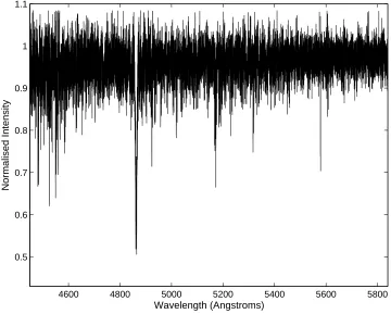
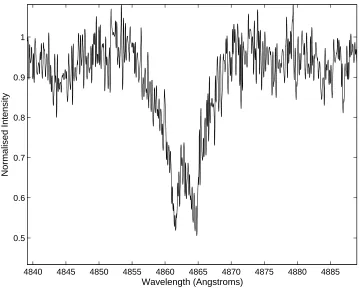
[image:47.595.127.487.408.697.2]

The observed spectra of V392 Car were taken over three months. The orders were ex-tracted by HRSP and the spectra were continuum fitted using a MATLAB script written by Duncan Wright (see appendix A). The continuum fitted orders were combined into one long spectrum using another MATLAB script from Duncan Wright (see appendix A). The process of combining the orders used non flat-fielded reduced images to get the mean at the cross-over regions and used these values to weight the flat-fielded reduced images which were then combined. Combining echelle orders gives a more informed cross correlation result as over the 2000˚A wavelength range there is a lot more information than with individual orders typically of the 50˚Arange. Figure 5.5 shows an example of a combined spectrum of V392 Car. The strong absorption line around 4860˚A is shown in Figure 5.6, it is the strongHβ line.

4600 4800 5000 5200 5400 5600 5800

0.5 0.6 0.7 0.8 0.9 1 1.1

Wavelength (Angstroms)

Normalised Intensity

Figure 5.5: The combined spectrum of V392 Car.

(48)

cor-36 CHAPTER 5. V392 CARINAE

4840 4845 4850 4855 4860 4865 4870 4875 4880 4885

0.5 0.6 0.7 0.8 0.9 1

Wavelength (Angstroms)

[image:48.595.100.459.123.412.2]

Normalised Intensity

Figure 5.6: The strong Hβ absorption line from fig 5.5.

rect for cosmic rays that were missed in the HRSP reduction. The long exposure times and poor signal to noise made the inbuilt HRSP cosmic ray extraction procedure less successful.

These spectra were then cross-correlated against a synthetic template spectrum (Tef f = 8750K, logg = 4.0), which was computed from ATLAS9 model atmospheres. The correlation is performed using the FFT technique in MATLAB. To prepare for the cross-correlation the combined spectra were scrunched to a constant logarithmic wavelength interval. The cross-correlation profiles produced defined peaks which were fitted with gaussians using FIGARO’s gauss program.

5.2.2 Radial Velocity Measurements

(49)

peaks were of gaussian form and were fitted with gaussians to determine the centroid of the peaks. FIGARO’s gaussian fitting packagegauss, provides an interactive fitting tool where the limits and position of the gaussian profile are specified. The resulting profile can then be modified in width, height and peak position, gauss then optimizes the gaussian given optional constraints.

The output measurement consists of the peak position, height and flux, along with the standard deviation of the gaussian profile (sigma) and the r.m.s. error on the fit. The CCFs were all plotted in velocity space and thus the measure of the peak gave direct radial velocities. The error estimate for all our measured radial velocities is 2kms−1

as explained in Section 3.4. The measured radial velocities were then corrected to air wavelengths using equation 3.6, and phased and separated into components in MATLAB.

−50 0 50 100 150 200 250

0.6 0.65 0.7 0.75 0.8 0.85 0.9 0.95 1 1.05 1.1

Velocity (km/s)

CCF normalised intensity

Figure 5.7: The cross-correlation function for V392 Car coming into an eclipse.

(50)

−50 0 50 100 150 200 250

0.6 0.65 0.7 0.75 0.8 0.85 0.9 0.95 1 1.05 1.1

Velocity (km/s)

[image:50.595.95.461.392.685.2]

CCF normalised intensity

Figure 5.8: The cross-correlation function of V392 Car near a time of maximum separation.

0 0.2 0.4 0.6 0.8 1 1.2 1.4 1.6 1.8 2

−100 −50 0 50 100 150

Phase

RV (km/s)

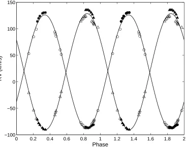
Figure 5.9: The Radial Velocity curves from both components of V392 Car including the

measurements from Debernardi and North (2001). Component one’s velocities are the tri-angles, circles are the velocities from component two, filled symbols are the radial velocities

(51)

5.3. ORBITAL ANALYSIS 39

5.3 Orbital Analysis

V392 Car is a SB2 type binary with eccentricity of zero. Therefore an orbital analysis from the measured radial velocities may be carried out using equation 3.7. The period of V392 Car was investigated with our measured radial velocities combined with the radial velocities from Debernardi and North (2001). The period used in Debernardi and North (2001) was not the best period for the velocity measurements. The best period was determined to beq = 3d_._1749749

±0.0000001. This period was used in PHOEBE to produce the model of best fit.

The spectroscopic orbital parametersγ,Kn,ansiniwere calculated from the fit of sine curves to the radial velocity curves. The fit was done in MATLAB using least-squares minimisation.

P 3d_.₁₄₉₇₄₉_±₀d_._0000001

e 0

γ1(kms−1) 19.057±0.130

γ2(kms−1) 18.787±0.129

γ(kms−1₎ ₁₈_.₉₂₂

±0.092

K1(kms−1) 109.635±0.173

K2(kms−1) 107.478±0.174

q = K2

K1 0.980±0.003

a1sini(R⊙) 6.882±0.011

a2sini(R⊙) 6.747±0.011

M1sin3i(M⊙) 1.667±0.005

[image:51.595.204.420.329.558.2]

M2sin3i(M⊙) 1.700±0.005

Table 5.1: The orbital elements of V392 Car.

5.4 Modeling with PHOEBE

V392 Car is a detached eclipsing binary. It’s light curve displays partial eclipses of similar depth. The HJD0, period and initial start points for the mass-ratio and temperatures

(52)

Primary Secondary

mass(M⊙) 1.915 1.862

radius(R⊙) 1.74 1.74

log(g) 4.24 4.23

[image:52.595.189.381.92.189.2]

a(R⊙) 7.103 6.825

Table 5.2: The absolute parameters of V392 Car.

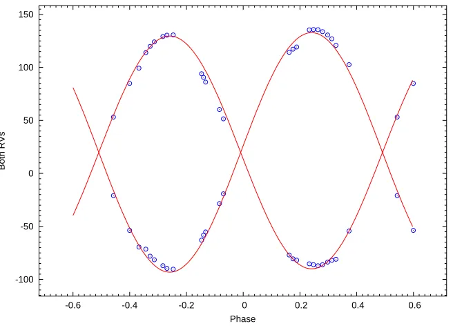
-100 -50 0 50 100 150

-0.6 -0.4 -0.2 0 0.2 0.4 0.6

Both RVs

Phase

Figure 5.10: The Radial Velocity curves from both components of V392 Car fitted with

the model generated in PHOEBE.

[image:52.595.120.448.256.492.2]

(53)

5.4. MODELING WITH PHOEBE 41

Parameter Solution

HJD0 2448000.55625

P 3d_._1749749

±0.0000001

q 0.951_±0.021

i 81.398_±0.195◦

Vγ(kms−1₎ ₁₉_.₇₉₂

±5.118

Semi₋majorAxis(R⊙) 14.000

T1( ◦

K) 8807_±100

T2( ◦

K) 8646_±97

Ω1 9.196±0.132

Ω2 8.856±0.156

g1 =g2 0.3

A1 0.909±0.733

A2 0.785±0.716

X1B 0.451_±1.25

X1Y 0.588_±1.07

X1V 1.018_±0.302

X2B 1.235_±0.184

X2Y 1.127_±0.375

X2V 1.064_±0.318

r1pole 0.121

r1point 0.122

r1side 0.121

r1back 0.122

r2pole 0.121

r2point 0.122

r2side 0.122

r2back 0.122

Σ(wr2₎ ₉_.₁₅

×10−4

σRV1(kms−1) 3.841

σRV2(kms−1) 4.933

Analysis of three close eclipsing binary systems: BP Velorum, V392 Carinae and V752 Centauri