Published online December 10, 2013 (http://www.sciencepublishinggroup.com/j/ijmsa) doi: 10.11648/j.ijmsa.20130206.17
Graphene in e
dge-carboxylated graphite
by ball milling
and analyses using finite element method
J. H. Lee
1, *, C. M. Shim
2, B. S. Lee
31
Dept. of Infrastructure Engineering, Chonbuk National University, Jeonju, South Korea 2
Dept. of Mechanical Engineering, Tohoku University, Tohoku, Japan 3
Dept. of Mathematics, University of Illinois, Urbana-Champaign, IL 61820, USA
Email address:
[email protected] (J. H. Lee), [email protected] (C. M. Shim), [email protected] (B. S. Lee)
To cite this article:
J. H. Lee, C. M. Shim, B. S. Lee. Graphene in Edge-Carboxylated Graphite by Ball Milling and Analyses Using Finite Element Method. International Journal of Materials Science and Applications. Vol. 2, No. 6, 2013, pp. 209-220. doi: 10.11648/j.ijmsa.20130206.17
Abstract:
Edge-carboxylated graphite (ECG) was produced by grinding pristine graphite in a planetary ball-mill machine. Transmission electron microscope was used to confirm the layers of graphene in ECG. The elemental analyses showed that the oxygen contents are different between ECG samples. The vibrational analysis of single- and five-layered graphene was conducted using finite element method within ANSYS. The vibrational behaviors of cantilevered and fixed graphene with one or five layerswere modeled using three-dimensional elastic beams of carbon bonds and point masses. The dynamic analysis was conducted using nonlinear elastic elements within LS-DYNA. The natural frequencies, strain and kinetic energy of the beam elements were calculated considering the van der Waals forces between the carbon atoms in the hexagonal lattice. The natural frequencies, strain and kinetic energy of the graphene sheets were estimated based on the geometrical type and the layered sheets with boundary conditions. In the dynamic analysis, the change in displacement over time appears larger along the x- and y-axes than along the z-axis, and the value of the displacement vector sum appears larger in the five-layer graphene than in the single-layer graphene.Keywords:
Edge-Carboxylated Graphite (ECG), Graphene, Van Der Waals Forces, Vibrational, Finite Element Method1. Introduction
Researchers worldwide have tried to estimate the mechanical properties of graphene in many ways including experimental, molecular dynamics (MD), and elastic continuum modeling approaches. Graphene is the basic structural unit of some carbon allotropes including graphite, carbon nanotubes and fullerenes [1]. It is believed to be composed of benzene rings stripped of their hydrogen atoms. The rolling-up of graphene along a given direction can produce a carbon nanotube. A zero-dimensional fullerene can also be obtained by wrapping-up graphene [2]. In 1940, it was theoretically established that graphene is the building block of graphite. In 2004, Geim et al. at Manchester University successfully identified single layers of graphene and other 2-D crystals [1, 4] in a simple tabletop experiment. These were previously considered to be thermodynamically unstable and unable to exist under ambient conditions [5].
Graphene can be prepared by four different methods [6]. The first is chemical vapor deposition (CVD) and epitaxial
growth, such as the decomposition of ethylene on nickel surfaces [3, 7]. The second is the micromechanical exfoliation of graphite, which is also known as the peel-off method by scotch tape [8]. The third method is epitaxial growth on electrically insulating surfaces, such as SiC, and the fourth is the solution-based reduction of graphene oxide [9].
SiO2 substrate [10-12].
Giannopoulos et al. [27] developed a finite element formulation that is appropriate for the computation of the Young’s and shear moduli of single-walled carbon nanotubes (SWCNTs). Zhang et al. [28] reviewed some basics in the use of continuum mechanics and molecular dynamics to characterize the deformation of single-walled carbon nanotubes (SWCNTs). Recently, several studies
[29-33] formulated the equations for an analytical solution using nonlocal elasticity theories. Ali Hemmasizadeh et al.
[34] developed an equivalent continuum model for a single-layered graphene sheet. This method integrates a molecular dynamics method as an exact numerical solution with theory of shells as an analytical method.
R. Ansari et al. [35] developed the vibrational characteristics of multi-layered graphene sheets with different boundary conditions embedded in an elastic medium for a nonlocal plate model that accounts for the small scale effects. Ragnar Larsson et al. [36] addressed the modeling of thin, monolayer graphene membranes, which have significant electrical and physical properties used for nano- or micro-devices, such as resonators and nanotransistors. The membrane is considered as a homogenized graphene monolayer on the macroscopic scale, and a continuum atomistic multiscale approach is exploited. Jia-Lin Tsai et al. [37] investigated the fracture behavior of a graphene sheet, containing a center crack, and characterized it based on atomistic simulation and continuum mechanics. Two failure modes, opening mode and sliding mode, were considered by applying remote tensile and shear loading, respectively, on the graphene sheet. S.K. Georgantzinos et al. [38] investigated the computation of the elastic mechanical properties of graphene sheets, nanoribbons and graphite flakes using spring-based finite element models. Interatomic bonded interactions as well as van der Waals forces between carbon atoms are simulated via the use of appropriate spring elements expressing corresponding potential energies provided by molecular theory.
The natural frequencies and mode shapes of the graphene layers in the edge-carboxylated graphite(ECG) under cantilevered and fixed boundary conditions was calculated in this study by applying a mass finite element model. An FEM modeling approach using ANSYS was implemented to achieve this result and to describe the graphene. Furthermore, FEM modeling for explicit dynamic analysis was approached using LS-DYNA.
2. Experimental Methods
Graphite power was purchased from Alfa Aesar (natural, 100 mesh, 99.9995 % metals basis, Lot#14735) and used as received. Dry ice was purchased from Fine Dryice Co., LTD, Korea. All other solvents were supplied by TaeMyong Scientific Co., LTD, Korea and used without further purification, unless otherwise specified. In a typical experiment, ball milling was carried out in a planetary
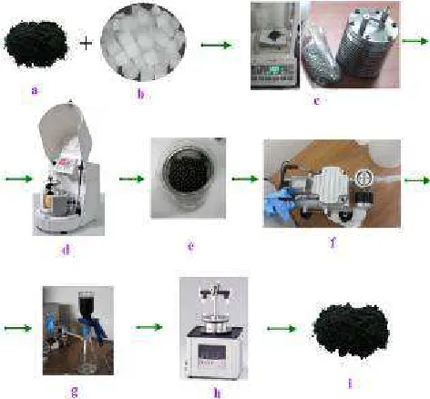
ball-mill machine (Pulverisette 6, Fritsch; Fig. 1d) in the presence of graphite (5.0 g, Fig. 1a), dry ice (100 g, Fig. 1b) and stainless steel balls (Fig. 1c).
Edge-carboxylation of graphite was prepared by ball milling of the pristine graphite in a planetary ball-mill machine in the presence of dry ice at 500 rpm. In a typical experiment, 5 g of the pristine graphite and 100 g of dry ice were placed into a stainless steel capsule containing stainless steel balls(300 ~ 320 g) of 5-mm diameter.
The capsule was then sealed and fixed in the planetary ball-mill machine, and agitated at 500 rpm for 48 h. The resultant product was further Soxhlet extracted with 1M aqueous HCl solution to completely acidify the carboxylates and to remove metallic impurities (Fig. 1g). Final product was freeze-dried by a freeze dryer(Fig. 1h) at −45°C under a reduced pressure for 48 h to yield 6.4 g of dark black powder(Fig. 1i) that the pristine graphite captured 1.4 g of CO2 during mechano-chemical cracking[13].
Fig 1. (a) Pristine graphite, (b) Dry ice, (c) Stainless steel capsule and balls, (d) Ball-mill machine, (e) Graphite prepared by ball milling with aqueous HCl solution, (f) Vacuum pump, (g) Vacuum filtering apparatus, (h) Freeze dryer, and (i) Final product ,Edge-carboxylated graphite (ECG).
The following explains the detail procedure for making ECG shown in Fig. 1.
1) Put graphite (5g) + dry ice (100g) + balls (300 ~ 320g) in the vessel and mix. Put graphite first and then the balls so that the graphite is not blown away.
2) Using a vacuum pump, remove the air inside the steel vessel. Good control is required when removing the air rapidly.
4) Open the vessel and filter the mixture of graphite and balls. Be mindful of the graphite powder blowing.
5) Put the resultant graphite mixture in 1 mol of HCl and leave for 48 hours. When mixing the graphite mixture with HCl, put 50mL of water, 25 mL of HCl and 200 mL of water successively. The concentration of HCl is around 38 %.
6) After 48 hours, filter the mixture with a vacuum filter. When filtering, divide the mixture's amount by around ten for divided filtering. Put distilled water into the divided mixtures and check the pH repeatedly until it becomes neutral. The filtering must not be done at once; if graphite is full on the filtering paper, it will take a great amount of time.
7) After filtering, freeze the mixture in a freezer, and then leave it in a freezing dryer for about one day.
Table 1. Elemental analysis of ECG samples after the ball milling for 48 hours
Sample C (%) H (%) N (%) O (%) S (%) C/O
Graphite[13] 99.64 BDL BDL 0.130 BDL 1021
ECG[13] 72.04 1.01 BDL 26.46 BDL 3.63
GO[13] 48.92 2.13 NA 45.45 NA 1.43
Jh-1 ECG 86.89 0.96 BDL 15.26 0.96 5.69
Jh-2 ECG 67.41 2.02 1.10 19.67 2.05 3.43
Jh-3 ECG 72.09 0.96 0 18.39 0 3.92
BDL = Below detection limit or not available. NA = Not applicable.
Table 1 shows the elemental analysis of ECG samples (Jh-1, Jh-2, Jh-3) after the ball milling for 48 hours. The detailed mechanism of carboxylation via mechano-chemical process by ball milling is presented elsewhere [13] and confirmed by various spectroscopic measurements.
Elemental analyses showed that the oxygen content has some differences between ECG samples after the ball milling for 48 hours. As shown in Table 1, the oxygen content of ECG samples(Jh-1, Jh-2, Jh-3) increased from 0.13 % to 15.6 %, 19.67 %, 18.39 % and 26.46 % [13]. In contrast, the carbon content of ECG samples decreased from 99.64 % to 86.89 %, 67.41 %, 72.09 % and 72.04 % [13]. The greater the oxygen content, the greater the graphene content is in the ECG samples. Elemental analyses showed that the oxygen content of ECG increased with an increase in the ball-milling times. The increase in the ball-milling time also caused a continuous decrease in the sample grain size until 48 h, when a steady state was reached, as seen in the high-resolution transmission electron microscope (HRTEM, JEOL JEM-2010) images in Fig. 2. Figs. 2a and b give typical HRTEM images of ECG made from the pristine graphite flake, showing nano-scale irregular particle grains with smooth surfaces. As proposed in Figs. 2c, d and e more homogenous but much smaller
ECG grains formed after ball milling for 48 h. The arrow shows layers of the graphene.
Figs. 1 and 2 show the HRTEM image of a typical multilayer graphene sheet on the lacey carbon-coated grid. Several folds can be seen in the MLG (Multi-layer graphene) sheets, which is typical in thin sheets of graphite. The MLG sheets had diameters generally between 500 and 2000 nm and were 1-10 graphene layers thick [14]. The weak contrast of the thin MLG sheet is apparent next to the strong contrast of the lacey carbon grid. The maximum number of layers is approximately 5, indicated by arrows. The corresponding HRTEM images are given in Fig. 3. Figs. 2c, d, e and Figs. 3c and d clearly show the presence of GNs. The ECG self-exfoliated into nanosheets in the dispersion used for the HRTEM sample preparation with wrinkle characteristics of flexible GNs.
Fig 2. HRTEM images obtained from randomly selected sample 1 ECGs at different magnifications: (a) 200 nm, (b) 100 nm, (c) 20 nm, (d) 10 nm, and (e) 5 nm. Maximum number of layers indicated by arrows is approximately 5.
Fig 3. HRTEM images obtained from randomly selected sample 2 ECGs at different magnifications: (a) 0.5µm, (b) 0.2µm, (c) 10 nm, and (d) 5 nm. Maximum number of layers indicated by arrows is approximately 5.
dispersion onto an HRTEM grid have a strong tendency to restack into overlapped aggregates[13]. Under higher magnification, the thin self-assembled ECG layer showed some edge distortion, as indicated by the arrow in Figs. 2c, d, e and Figs. 3c and d. As observed in HRTEM (Fig. 2, 3), most of the GN layers were typically less than five graphitic layers. These results clearly indicate that the pristine graphite flakes could have been directly exfoliated into few-layer GNs by ball milling in the presence of dry ice, followed by dispersion in polar solvents. From EA data (i.e., an oxygen content of 15.26 %, 19.67 %, 18.39 % and C/O = 5.69, 3.43, 3.92, Table 1) for ECG ball milled for 48h, it can be estimated that an average of one carboxylic acid group has been introduced onto every 11.38, 6.86 and 7.84 carbons along the distorted ECG edge if there is negligible carboxylation on the basal plane [13].
Therefore, the ball milling method, which requires neither hazardous chemicals nor tedious procedures, outperforms current methods for mass production of high-quality GNs at low cost.
3. Simulation of Molecular Bonds by
VDW
GNs were treated as a frame structure in which their bonds were beam members and carbon atoms were joints. To establish the linkage between the force constants in molecular mechanics and the beam element stiffness in structural mechanics, the energy equivalence concept proposed by Li et al.[18] was employed.
In general, the total steric potential energy of the force field in MD can be expressed as the sum of the energies of bonded and nonbonded interactions [19] as:
total r vdw
U
=Σ +Σ +Σ +Σ +Σ
U
U
θU
ϕU
ωU
(1)where Ur, Uθ, Uφ, Uω, and Uvdw are the energies for bond stretching, bond angle bending, dihedral angle torsion, out-of-plane torsion, and nonbonded van der Waals interactions, respectively.
The van der Waals force is an intermolecular force that arises from a fluctuating electromagnetic field resulting in instantaneous electrical and magnetic polarizations between atoms and molecules. The van der Waals force has been studied extensively [16, 20]. Yang et al. [22] have developed a non-uniform rational B-spline (NURBS) surface approach for van der Waals force computation. In a system of two carbon atom spherical particles 1 and 2 of radii r1 and r2[23] with a separation of d, the non-retarded van der Waals force between two spheres is provided by Chen et al.[15]:
(
)
(
)
(
)
1 2
2
1 2 1 2 1/ 4 2 1 2 1 2 1 2 1 2 12 / 3
1/ 2 1/ 4 /8 S
F A d r r
d r r r r+ d r r r r rr r r r r
= − + +
− + + + +
+
(2)
From (2), three geometric parameters, the separation
distance d and sphere radii r1 and r2, are required to calculate the van der Waals forces for sphere–sphere interaction. In this case, we adopt the same separation distance d =2.442 nm and fix the sphere radii as r1 = r2 = 0.07 nm and Hamaker constant A = 0.284e-19.
Chen et al.[15] also obtained closed-form solutions for sphere-half and sphere-sphere systems. Consider a system of two spheres 1 and 2 of radii r1 and r2, respectively, placed at a center-to-center separation distance of h. Here, d is the closest separation between the spheres. The van der Waals attractive force F(h) is given by:
( )
0( ) ( )
1F h =A F h +F h (3)
Where
( )
2 2 2 20 /3 1/ 1 3 1/ 2 4 21 2/ 1 3 21 2/ 2 4
F h=h − d d+ d d+ rr d d +rr d d (4)
(5)
From (5),
1 1 2, 2 1 2, 3 1 2, 4 1 2
d = − −h r r d = + −h r r d = + +h r r d = − +h r r and
( 1) 4 3
1 2
, ( 1)i [4 5( )] 20 ,
i i i i i i
e =d +c b = − + e e − h c+ − r r e
(
)
( )
1 3 2 2
1 2
( 1)i 4 5 4 20 20 (3 )
i i i i i i
g= − +e e − h c e+ + h h c+ + rr e h e− .
Israelachvili [17] reported that for interatomic van der Waals forces, (6) is the force for two atoms or small molecules, and (7) is the force for two spheres or macromolecules. C is the coefficient in the atom-atom pair potential :
7 6 /
F= − C r (6)
(
2)
[
]
2 1
1 2
6 ( )
F= −A d r r r +r (7)
Kalamkarov et al. [22] stated that the non-covalent interactions such as van der Waals forces, can be adequately described using the Lennard–Jones potential. The corresponding energy can be expressed by:
(
) (
12)
64 12 / /
LJ
V = ε− σ r + σ r (8)
(
) (
12)
6/ 4 / 12 / /
LJ LJ
F =dV dr= ε r− σ r +σ r (9)
where σ = 0.34 nm and ε = 0.0556 Kcal/mol.
Each van der Waals force in (3), (6), (7) and (9) is calculated as an equivalent value to the variable applied to the mode analysis of nanocones represented in (2). We adopt the same separation distance of h=2.582 nm. The van der Waals force calculated in (2) is equal to 812.993 N, and that calculated in (3) was -2.882e-08 N; (6) yielded -0.045e-75 N and (7) yielded -0.278e-24 N, and (9) yielded 4.49e-06 N. The values in (3), (6), (7) and (9) are ignored since they are too small, and the value in (2) is used.
4. Implementation of the Finite Element
Model
Based on the modeling concept described, the finite element model for single and five-layer graphene was implemented using commercial ANSYS software. First, we will briefly summarize the simulating element type used in ANSYS for the problem considered. The C–C bonds were simulated as BEAM188 beam elements, and the carbon atoms were simulated as MASS21 mass elements.
Fig 4. Finite element model of single and five-layer graphene.
Concentrated masses were used to model carbon atoms as point elements with up to six degrees of freedom, and translations in the nodal x, y, and z directions and rotations about the nodal x, y, and z axes. A different mass and rotary inertia could be assigned to each coordinate direction. The mass element was defined as a single node, concentrated mass components in the element coordinate directions, or rotary inertias about the element coordinate axes. The element coordinate system was initially parallel to the global Cartesian coordinate system or to the nodal coordinate system and rotated with the nodal coordinate rotations during the large deflection analysis. If the element required only one mass input, it was assumed to act in all appropriate coordinate directions. The mass element had no
effect on the static analysis solution unless acceleration or rotation was present [23]. Five-layer graphene was modeled with 0.35nm spacing from single-layer graphene along the z-direction. As an example, the established finite element models of single-layer graphene and five-layer graphene was shown in Fig. 4, respectively.
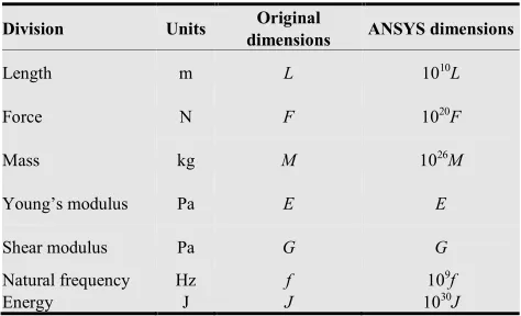
Before we input the data of the BEAM188 and MASS21 element properties, the dimensions of the parameters stated above were further adjusted to avoid possible flow errors during the ANSYS computation. Thus, the dimensions were adjusted as shown in Table 2 [24]. After adjustment, the numerical parts of the input data were prepared for the BEAM188 and MASS21 elements, as shown in Table 3[24].
Table 2. Adjusted dimensions for ANSYS.
Division Units Original
dimensions ANSYS dimensions
Length m L 1010L
Force N F 1020F
Mass kg M 1026M
Young’s modulus Pa E E
Shear modulus Pa G G
Natural frequency Energy
Hz J
f J
109f 1030J
Table 3. The input data prepared for the BEAM188 and MASS21 elements.
Division Units ANSYS dimensions Values
C-C bond diameter m D 0.1466
Poisson's ratio ν 0.3
Density kg/m3 ρ 2.3e3
Young’s modulus Pa E 5.448e12
Shear modulus Pa G 0.8701e12
Mass of carbon atom kg Mc 2.0
After ANSYS mode analysis, we found the node with the maximum strain and kinetic energies from modes 5, 10, 15 and 20 of each graphene sheet. Then, in order to determine the accurate displacement about the x-, y- and z- axes of the node, we conducted explicit dynamic analysis in LS-DYNA after the second FEM modeling.
5. Vibrational and Dynamic Analysis
5.1. Vibrational Analysis Using ANSYS
mass system. The generalized equation of motion is given as follows [23]:
[ ]
M{ }
uɺɺ +[ ]
C u{ }
ɺ +[ ]
K{ }
u =[ ]
F (10)where [M] is the mass matrix,
{ }
uɺɺ is the second time derivative of the displacement{ }
u (i.e., the acceleration),{ }
u
ɺ
is the velocity, [C] is a damping matrix, [K] is the stiffness matrix, and [F] is the force vector.Vibrational analysis was used for natural frequency and mode shape determination. For vibrational analysis, damping was generally ignored. The equation of motion for an undamped system, expressed in matrix notation, is given in (11):
[ ]
M u
{ }
ɺɺ
+
[ ]
K u
{ } { }
=
0
(11)Note that
[ ]
K , the structure stiffness matrix, may include pre-stress effects. For a linear system, free vibrations will be harmonic with the following form:{ } { }
cos
i iu
=
ϕ
ω
t
(12)where {φ}i , ωi , and t are the vectors representing the mode shape of the ith natural frequency, the ith natural circular frequency (radians per unit time), and time, respectively. Thus, (11) can be rewritten as:
[ ] [ ]
{ } { }
2
(
i)
0
i
M
K
ω
ϕ
−
+
=
(13)This equality is satisfied if either {φ}i = {0} or if the determinant of ([K] - ω2 [M]) is zero. The first option is trivial and is therefore not of interest. The second gives the following solution:
[ ]
2[ ]
0
K −ω M = (14)
This is an eigenvalue problem that can be solved for up to n values of ω2 and n eigenvectors {φ}i which satisfy
(19)
, where n is the number of DOFs. The eigenvalue andeigenvector extraction techniques are used in the Block Lanczos method. Rather than outputting the natural circular frequencies {ω}, the natural frequencies (f) are output as
/ 2
i i
f =ω π (15)
where fi, is the ith natural frequency (cycles per unit time). Normalization of each eigenvector {φ}i to the mass matrix is performed according to
{ }
ϕiT[ ]
M{ }
ϕi=0 (16)In the normalization, {φ}i is normalized such that its largest component is 1.0 (unity).
The natural frequency of a structure is related to its geometry, mass, and boundary conditions. For the graphene
sheets considered here, the mass was assumed to be that of each carbon atom, 2.0×10⁻²⁶ kg, and the rotational degrees of freedom of the atoms were neglected due to their extremely small diameter. In terms of the boundary conditions, one end of the graphene sheets was fixed, and the other was free as a cantilever type. These conditions were also true for the second explicit dynamic analysis.
5.2. Dynamic Analysis Using LS-DYNA
Consider the single degree of freedom damped system with forces acting on mass m for time integration. The equilibrium equations are obtained from d'Alembert’s principle as [23, 25]:
( )
I D S
f
+
f
+
f
=
p t
(17)where c is the damping coefficient, and k is the linear stiffness. For critical damping
c c
=
cr, the equations ofmotion for linear behavior lead to a linear ordinary differential equation:
( )
mu cu kuɺɺ+ +ɺ = p t , (18)
But, for the nonlinear case, the internal force varies as a nonlinear function of the displacement, leading to a nonlinear ordinary differential equation:
( )
S( )
mu cu f u
ɺɺ
+ +
ɺ
=
p t
(19)Analytical solutions of linear ordinary differential equations are available, so we instead consider the dynamic response of a linear system subjected to a harmonic loading. It is convenient to define some commonly used terms:
Harmonic loading: p t
( )
=p0sinωt, Circular frequency:/ k m
ω= for a single degree of freedom, Natural frequency: f =ω π2 =1 / ,T T= period , Damping ratio: ξ =c c/ cr =c/ 2mω , Damped vibration
frequency: 1 2
D
ω =ω −ξ , Applied load
frequency:β ω ω= / .
The dynamic response of a linear undamped system due to harmonic loading is:
(20)
for the initial conditions: u0 = initial displacement, uɺ0 = initial velocity, p0/k = static displacement, and
2
uses the explicit central difference time integration method [26] to integrate the equations of motion.
6. Numerical Results
6.1. Vibrational Analysis Results
The single and five-layer graphene with cantilevered and fixed type boundary conditions were modeled using 3-D beam and mass elements. The graphene sheets were produced by ball milling pristine graphite in the presence of dry ice. The numerical results of the graphene sheets are given in Tables 4 and 5 and in Figs. 5 and 6.
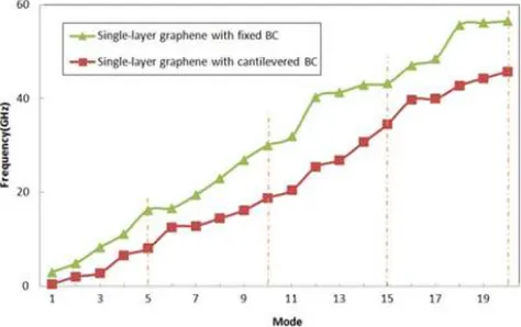
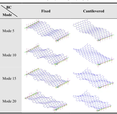
The deformed shapes of modes 5, 10, 15, and 20 for the single and five-layer graphene with the boundary conditions are illustrated in Tables 4 and 5. The variations in frequency versus the mode of vibration for the single and five-layer graphene was compared in Figs. 5 and 6. As shown, the frequency increased when the single-layer graphene, without respect to the boundary conditions.
As can be seen, the frequency did not significantly differ for the modes of five-layer graphene as for the boundary conditions; however, a regular pattern of variation was observed at higher vibrations such that the curves of variation for the graphene sheets with a cantilever increased at all points.
The results illustrated in Fig. 5 for the single-layer graphene display the same trend as that observed for the five-layer graphene in Fig. 6. It can be deduced from the figure that the natural frequency increases with the mode number, and the increase in the natural frequency of the single-layer graphene is approximately five times that of the five-layer graphene. The modes of deformation illustrated in the tables show that the five-layer graphene undergo bending as does the single-layer graphene with a different trend pattern.
From the comparison of the vibrational modes illustrated in Figs. 5 and 6 for the graphene sheets of different boundary conditions, it can be concluded that the modes are mainly the sum of the translation and rotation modes. These two modes are enlarged in the figures with greater mode number.
As indicated by Tables 4 and 5, the severity of deformation varied among the graphene sheets with different boundary conditions. It is also evident that the natural frequency of the single-layer graphene with cantilevered boundary condition shown in Fig. 5 was lower than those with fixed boundary condition. The natural frequency of the five-layer graphene with cantilevered boundary condition shown in Fig. 6 was lower than those with fixed boundary condition.
In the fifth mode in Tables 4 and 5, the deformed and initial graphene sheets overlap considerably so that the deformed sheet lies inside the initial sheet, whereas the deformed and initial graphene sheets for the tenth, fifteenth
and twentieth modes of deformation shown in Tables 4 and 5 overlap with some interference only at the free end of the graphene sheets. The other modes of deformation can be explained in a similar manner. Therefore, as in Figs. 5 and 6, the numerical results indicate that the graphene sheets underwent slight deformation and vibration as the number of graphene layers increased.
Fig 5.Variation in the natural frequency of the single-layer graphene with cantilevered and fixed boundary conditions.
Table 4. Mode shapes of the single-layer graphene.
BC Mode
Fixed Cantilevered
Mode 5
Mode 10
Mode 15
Mode 20
Table 5. Mode shapes of the five-layer graphene.
BC
Mode Fixed Cantilevered
Mode 5
Mode 10
Mode 15
Mode 20
The potential energy including the strain energy of elements is:
1 / 2
po e
E =
{ }
U
e T(
K
e
+
S
e)
{ }
U
e
(21)and the kinetic energy computed only for modal analyses is:
1 / 2
ki e
E =
{ }
{ }
T
e e e
U
M
U
ɺ
ɺ
(22)where
K
e
is the element stiffness matrix,
S
e is theelement stress stiffness matrix,
{ }
U
e is the element DOFFig 7. Strain energies for the single-layer grapheme ith cantilevered boundary condition.
vector,
{ }
U
ɺ
e is the time derivative of the element DOFvector, and
M
e
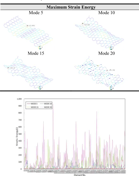
is the element mass matrix[23].Table 6 shows a comparison of the single-layer graphene with cantilevered boundary condition for maximum strain energies of modes 5, 10, 15, and 20. Table 7 shows a comparison of the single-layer graphene with fixed boundary condition for maximum strain energies. As can be observed in Table 6, for the cantilevered single-layer graphene, the maximum value of the strain energies was in element no. 299 at mode 20 (671.33 J, see Fig. 7), and the maximum value of the kinetic energies was in element no. 96 at mode 20 (929.20 J, see Fig. 8). As can be observed in Table 7, for the fixed single-layer graphene, the maximum value of the strain energies was in element no. 13 at mode 20 (1032.69 J, see Fig. 9), and the maximum value of the kinetic energies was in element no. 4 at mode 20 (2084.30 J, see Fig. 10).
For the cantilevered five-layer graphene, the maximum value of the strain energies was in the third layer at mode 20 (5.95 J, see Table 8), and for the fixed five-layer graphene, the maximum value of the strain energies was in the second layer at mode 20 (25.01 J, see Table 9).
Table 6. Maximum strain energies for the single-layer grapheme with cantilevered boundary condition.
Maximum Strain Energy
Mode 5 Mode 10
Mode 15 Mode 20
Fig 8. Kinetic energies for the single-layer graphene with cantilevered boundary condition.
Table 7. Maximum strain energies for the single-layer graphene ith fixed boundary condition.
Maximum Strain Energy
Mode 5 Mode 10
Mode 15 Mode 20
Fig 9. Strain energies for the single-layer graphene with fixed boundary condition.
Fig 10. Kinetic energies for the single-layer graphene with fixed boundary condition.
Table 8. Maximum strain energies for the five-layer graphene with cantilevered boundary condition.
Maximum Strain Energy
Mode 5 Mode 10
Mode 15 Mode 20
Table 9. Maximum strain energies for the five-layer graphene with fixed boundary condition.
Maximum Strain Energy
Mode 5 Mode 10
Mode 15 Mode 20
6.2. Dynamic analysis results
The second dynamic analysis results are shown in Figs. 11 and 12 for the single- layer graphene and Figs. 13 and 14 for the five-layer graphene. The explicit dynamic analysis in LS-DYNA after the second FEM modeling is conducted for 20 seconds.
The values of displacements and displacement vector sums along the x-, y- and z-directions at the chosen nodes are shown in each figure. In Figs. 11 and 12, the displacements along the x- and y-directions have somewhat large variations, but the displacement along the z-direction is essentially zero.
A similar phenomenon also appears in Figs. 13 and 14 for the five-layer graphene sheets. The single and five-layer graphene have larger variations in displacement as time passes. It is shown that the displacement variation is especially great in the y-direction. Overall, the values of a displacement vector sum, which is indicated as DMX in the figures, appears smaller in the single-layer graphene than in the five-layer graphene.
The increase along the x- and y-directions was regular at fewer displacements, but was irregular with more. The increases in the pattern of variation of the displacement for the fixed single and five-layer graphene were more regular at fewer displacements than that for the cantilevered single and five-layer graphene. This is closely related to the boundary conditions of the graphene sheets.
Fig 11. Displacements and displacement vector sum in node 3 of the single-layer graphene with cantilevered boundary condition.
Fig 12. Displacements and displacement vector sum in node 35 of the single-layer graphene with fixed boundary condition.
Fig 13. Displacements and displacement vector sum in node 304 of the five-layer graphene with cantilevered boundary condition.
Fig 14. Displacements and displacement vector sum in node 380 of the five-layer graphene with fixed boundary condition.
7. Conclusions
The vibrational and dynamic behavior of the single-layer graphene and those of the five-layer graphene with two different boundary conditions were studied using a finite element method comprised of beam and mass elements in a three-dimensional coordinate system. In order to explore the vibrational behavior, the influences of layered graphene sheets on the natural frequencies of the cantilevered and fixed boundary conditions were considered. The dynamic behavior was interpreted and analyzed by additional FEM modeling regardless of nodes selected in mode analysis.
Generally speaking, the computational results of the graphene sheets do not seem to be in good agreement with the existing data in the literature because of the difference of analysis methods.
The decrease in the number of layered sheets for graphene resulted in an increase in frequency. The decrease, however, was not severe for the first two modes of the single-layer graphene and for the first ten modes of the five-layer graphene. The modes of deformation illustrated in Tables 4 and 5 show that the single-layer graphene underwent more deformation with decreased number of atoms and bonds than did the five-layer graphene.
Therefore, the increase in the number of layered sheets for graphene can produce more structural equilibrium.
The results imply that the stable frequency of the graphene sheets is dependent on the boundary conditions and the number of layered sheets at all modes of vibration.
In the dynamic analysis, the displacement along the y-axis shows the greatest variation, and the value of the displacement vector sum appears larger with the five-layer graphene than with the single-layer graphene. This is thought to be related to mass.
Acknowledgments
This paper was supported by the research funds of Chonbuk National University, 2012.
References
[1] A.H. Castro Neto, F. Guinea, N.M.R. Peres, “Drawing conclusions from graphene,” Physics World 19, 2006, pp. 33-7.
[3] K. Kinghong, W.K.S. Chiu, “Growth of carbon nanotubes by open-air laser-induced chemical vapor deposition,” Carbon 43, 2005, pp. 437–446.
[4] P. Nemes-Incze, Z. Osváth, K. Kamarás, L.P. Biró, “Anomalies in thickness measurements of graphene and few layer graphite crystals by tapping mode atomic force microscopy,” Carbon 46, 2008, pp. 1435 –1442.
[5] L.D. Landau, E.M. Lifshitz, Statistical physics Part I, 3rd ed. Oxford, England Pergamon Press, 1980.
[6] S. Park, R.S. Ruoff, “Chemical methods for the production of graphenes,” Nature Nanotechnology l 4, 2009, pp. 217–224.
[7] D.R. Dreyer, S. Park, C.W. Bielawski, R.S. Ruoff, “The chemistry of graphene oxide,” Chem. Soc. Rev. 39, 2010, pp. 228–240.
[8] M. Izenberg, J.M. Blakely, “Carbon monolayer phase condensation on Ni(III),” Surf. Sci. 82, 1979, pp. 228-36.
[9] X. Lu, M. Yu, H. Huang, R.S. Rouff, “Tailoring graphite with the goal of achieving single sheets,” Nanotechnology 10, 1999, pp. 269-72.
[10] C. Berger, Z. Song, X. Li,X. Wu, N. Brown, C. Naud, D. Mayou, T. Li, J. Hass, A.N. Marchenkov, E.H. Conrad, P.N. First, W.A. de Heer, “Electronic confinement and coherence in patterned epitaxial graphene,” Science 312, 2006, pp. 1191-6.
[11] C.D. Reddy, S. Rajendran, K.M. Liew, “Equilibrium configuration and continuum elastic properties of finite sized graphene,” Nanotechnology 17, 2006, pp. 864-70.
[12] D.W. Boukhvalov, M.I. Katsnelson, A.I. Lichtenstein, “Hydrogen on graphene: electronic structure, total energy, structural distortions and magnetism from first-principles calculations,” Phy. Rev. B 77, 2008, 035427-1-7.
[13] In-Yup Jeon, Yeon-Ran Shin, Gyung-Joo Sohn, Hyun-Jung Choi, Seo-Yoon Bae, Javeed Mahmood, Sun-Min Jung, Jeong-Min Seo, Min-Jung Kim, Dong Wook Chang, Liming Dai, Jong-Beom Baek, “Edge-carboxylated graphene nanosheets via ball milling,” Proc. Nat. Acad. Sci. USA 109, 2012, pp. 5588-5593.
[14] J.H. Warner, F. Schäffel, M.H. Rümmeli, B. Büchner, “Examining the Edges of Multi-Layer Graphene Sheets,” Chem. Mater. 21, 2009, pp. 2418–2421.
[15] J. Chen, A. Anandarajah, “Van der Waals Attraction between Spherical Particles,” J. of Colloid Interface Science 180, 1996, pp. 519-523.
[16] J.N. Israelachvili, “The nature of van der waals forces,” Contemporary Physics 15 (2), 1974, pp. 159-178.
[17] J.N. Israelachvili, Van der Waals Forces between Particles and Surfaces, Intermolecular and Surface Forces (Third Edition) Ch.13, 2010, Academic Press.
[18] C. Li, T.W. Chou, “A structural mechanics approach for the analysis of carbon nanotubes,” Int. J. Solids Struct. 40, 2003, pp. 2487.
[19] M. Meo, M. Rossi, “Prediction of Young’s modulus of single wall carbon nanotubes by molecular-mechanics based finite element modelling,” Composites Science and Technology 66, 2006, pp. 1597–1605.
[20] S.W. Montgomery, M.A. Franchek, V.W. Goldschmidt, “Analytical Dispersion Force Calculations for Nontraditional Geometries,” J. of Colloid Interface Science 227 (2), 2000, pp. 567–584.
[21] P. Yang, X. Qian, “A general, accurate procedure for calculating molecular interaction force,” J. of Colloid and Interface Science 337, 2009, pp. 594–605.
[22] A.L. Kalamkarov, A.V. Georgiades, S.K. Rokkam, V.P. Veedu, M.N. Ghasemi-Nejhad, “Analytical and numerical techniques to predict carbon nanotubes properties,” Int. J. Solid Struct. 43, 2006, pp. 6832–54.
[23] J.H. Lee, B.S. Lee, F.T.K. Au, J. Zhang, Y. Zeng, “Vibrational and dynamic analysis of C60 and C30 fullerenes using FEM,” Comput. Mater. Sci. 56, 2012, pp. 131-140.
[24] J.H. Lee, B.S. Lee, “Modal analysis of carbon nanotubes and nanocones using FEM,” Comput. Mater. Sci. 51, 2012, pp. 30-42.
[25] J.O. Hallquist, LS-DYNA Theoretical Manual, Livermore Software Technology Corporation, 2006.
[26] Y. Liu, “ANSYS and LS-DYNA used for structural analysis,” Int. J. Computer Aided Engineering and Technology 1 1 , 2008, pp. 31-44.
[27] G.I. Giannopoulos, P.A. Kakavas, N.K. Anifantis, “Evaluation of the effective mechanical properties of single walled carbon nanotubes using a spring based finite element approach,” Comput. Mater. Sci. 41, 2008, pp. 561-569.
[28] L.C. Zhang, “On the mechanics of single-walled carbon nanotubes,” J. of Materials Processing Technology 209, 2009, pp. 4223–4228.
[29] E.Jomehzadeh, A.R. Saidi, “Decoupling the nonlocal elasticity equations for three dimensional vibration analysis of nano-plates,” Composite Structures 93, 2011, pp. 1015–1020.
[30] J.N. Reddy, “Nonlocal theories for bending, buckling and vibration of beams,” Int. J. of Engineering Science 45 ,2007, pp. 288–307.
[31] T. Murmu, S.C. Pradhan, “Small-scale effect on the vibration of nonuniform nanocantilever based on nonlocal elasticity theory,” Physica E 41, 2009, pp. 1451–1456.
[32] R. Ansari, H. Ramezannezhad, “Nonlocal Timoshenko beam model for the large-amplitude vibrations of embedded multiwalled carbon nanotubes including thermal effects,” Physica E 43, 2011, pp. 1171–1178.
[33] S. Narendar, D. Roy Mahapatra, S. Gopalakrishnan, “Prediction of nonlocal scaling parameter for armchair and zigzag single-walled carbon nanotubes based on molecular structural mechanics, nonlocal elasticity and wave propagation,” Int. J. of Engineering Science 49, 2011, pp. 509–522.
[34] Ali Hemmasizadeh, Mojtaba Mahzoon, Ehsan Hadi, Rasoul
Khandan, “A method for developing the equivalent
continuum model of a single layer graphene sheet,” Thin Solid Films 516, 2008, pp. 7636–7640.
[36] Ragnar Larsson, Kaveh Samadikhah, “Atomistic continuum modeling of graphene membranes,” Comput. Mater. Sci. 50, 2011, pp. 1744-53.
[37] Jia-Lin Tsai, Shi-Hua Tzeng, Yu-Jen Tzou, “Characterizing the fracture parameters of a graphene sheet using atomistic simulation and continuum mechanics,” Int. J. of Solids and Structures 47, 2010, pp. 503–509.