SCALABLE, DETERMINISTIC AND UPDATABLE FLOW PROCESSING FRAMEWORK TO ACCELERATE SOFTWARE DEFINED NETWORKING
By HAI SUN
A dissertation submitted in partial fulfillment of the requirements for the degree of
DOCTOR OF PHILOSOPHY
WASHINGTON STATE UNIVERSITY
School of Electrical Engineering and Computer Science MAY 2015
To the Faculty of Washington State University:
The members of the Committee appointed to examine the dissertation of HAI SUN find it satisfactory and recommend that it be accepted.
Min Sik Kim, Ph.D., Chair
Carl H. Hauser, Ph.D.
David E. Bakken, Ph.D.
ACKNOWLEDGEMENTS
First of all I would like to acknowledge my research adviser Dr. Min Sik Kim, who guided me to accomplish my graduation. His great patience and diligent mentoring throughout my PhD program encouraged and inspired me along the forward road. Only with the opportunity and resources he provided as well as his insightful opinions in research, I could accomplish the disser-tation.
I would like to thank Yan Sun for his tremendous help in every aspect of my research. His incisive intuition and insights in the networking area were really inspiring. I highly appreciate his time and discussion during the past years.
I acknowledge the other two Network Research Lab group members, Vic and Haiqin for their individual help to my graduate work.
It has been an honor to have Dr. Carl H. Hauser, Dr. David E. Bakken and Dr. Ananth Kalyanaraman in my Ph.D. research committee. I appreciate their time and effort before and during my dissertation work.
Eventually I would like to offer my most heartfelt appreciations to my parents and my wife Yanrong for their love throughout my life. Especially I am grateful to their inspiration, uncondi-tional support and encouragement during my dissertation work. I would like to thank my aunt and uncle for their care and help, and thank dear Kelsey and Jerry for every happy moment.
SCALABLE, DETERMINISTIC AND UPDATABLE FLOW PROCESSING FRAMEWORK TO ACCELERATE SOFTWARE DEFINED NETWORKING
Abstract by Hai Sun, Ph.D. Washington State University
May 2015
Chair: Min Sik Kim
To accomplish high-performance and granular traffic control across a great number of net-work devices, flow processing in an OpenFlow switch is of great importance for any Software Defined Networking (SDN) architecture. The fundamental challenge is to classify incoming pack-ets efficiently according to a pipeline of flow tables characterized by numerous fields and match types. So far current packet classification algorithms is not able to process a flow table with an arbi-trary number of fields and any match type due to several crucial drawbacks, especially scalability, incremental update and nondeterminism. To address the new challenge we propose an innovative decomposition algorithm.
Meanwhile we propose three different schemes to process flow tables with only exact match, prefix match and classic quintuple match. They are (1) a highly deterministic hashing scheme featured by efficient collision resolution, (2) a hierarchical hashing scheme featured by taking advantage of bitmap and hashing techniques, and (3) a divide-and-conquer scheme based on Ternary Content Addressable Memory (TCAM) hardware by addressing the range expansion problem. Together with the proposed decomposition algorithm, these four approaches cover all categories of match types and comprise a high-performance table lookup accelerator to boost flow processing in an OpenFlow switch.
As far as we know, our proposed decomposition scheme is the first efficient approach to addressing multidimensional match problem in an OpenFlow flow table with an arbitrary number of fields and any match type. And our proposed high-performance table lookup accelerator is the first comprehensive proposal to process the entire OpenFlow table pipeline by covering all categories of match types and any number of fields. The accelerator is available to be implemented and deployed in either software or hardware devices with respect to a variety of performance and cost circumstances.
TABLE OF CONTENTS Page ABSTRACT . . . iv LIST OF TABLES . . . x LIST OF FIGURES . . . xi CHAPTER 1 Introduction . . . 1
2 Highly Deterministic Hashing Scheme Using Bitmap Filter . . . 9
2.1 Background . . . 9
2.2 Related Work . . . 11
2.3 DOhashing andBHhashing . . . 12
2.3.1 DOhashing . . . 12 2.3.2 BHhashing . . . 17 2.4 Hierarchy Design . . . 19 2.4.1 Load Analysis . . . 21 2.4.2 Dimension Assignment . . . 23 2.4.3 Query . . . 24 2.5 Simulation . . . 26 2.5.1 Re-balance Influence . . . 27 2.5.2 Update Efficiency . . . 28
2.5.3 Memory Evaluation and Filter Comparison . . . 29
2.6 Summary . . . 30
3.1 Introduction to IP address lookup . . . 32
3.2 Background . . . 33
3.3 Scheme Details . . . 35
3.3.1 Observations and Ideas . . . 35
3.3.2 Two-Layer Hierarchy . . . 37
3.4 Preprocessing, Lookup and Update . . . 40
3.4.1 Preprocessing Algorithm . . . 40
3.4.2 Lookup Algorithm . . . 40
3.4.3 Update Algorithm . . . 42
3.5 Performance Evaluation . . . 43
3.5.1 Theoretical Analysis . . . 43
3.5.2 Evaluation using Real Routing Tables . . . 48
3.5.3 Discussion . . . 52
3.6 Summary . . . 54
4 TCAM-Based Classification Using Divide-and-Conquer for Range Expansion . . . 56
4.1 Introduction to Packet Classification . . . 56
4.1.1 Software-based Algorithms . . . 57
4.1.2 TCAM-based Algorithms . . . 58
4.2 Background . . . 60
4.3 DCS Design . . . 63
4.3.1 Problem Statement and Overview . . . 63
4.3.2 Start Point: Worst-Case Scenario . . . 68
4.3.3 Divide and Conquer . . . 69
4.3.5 Recursive DCS . . . 76
4.4 Evaluation . . . 83
4.4.1 Theoretical Analysis . . . 83
4.4.2 Evaluation using Synthetic Packet Classifiers . . . 85
4.5 Summary . . . 93
5 OpenFlow Accelerator: A Decomposition-based Hashing Approach for Flow Processing 94 5.1 Background . . . 94
5.2 Related Work . . . 97
5.3 Multidimensional Flow Processing . . . 100
5.3.1 Problem Statement . . . 100 5.3.2 Overview . . . 102 5.3.3 Preprocessing . . . 105 5.3.4 Query . . . 109 5.3.5 Update . . . 111 5.4 Evaluation . . . 113 5.4.1 Theoretical Comparison . . . 113
5.4.2 Implementation and Measurement . . . 115
5.5 Summary . . . 123
6 Flow Processing Accelerator . . . 124
6.1 Framework Overview . . . 124
6.2 Performance Evaluation and Analysis . . . 126
6.2.1 Search Time . . . 127
6.2.2 Memory Consumption . . . 128
6.2.4 Updatability . . . 130
6.2.5 Determinism . . . 131
7 Conclusion . . . 132
LIST OF TABLES
1.1 OpenFlow Required Field Table . . . 3
2.1 8-table Hierarchy . . . 23
2.2 Comparison Results . . . 29
3.1 An IPv4 Routing Table . . . 34
3.2 Search Time per IPv4 Packet (µs) . . . 51
4.1 A Simple Packet Classifier . . . 60
4.2 Comparison of Key Metrics for Range Encoding Schemes . . . 83
4.3 Range Statistics in Packet Classifiers . . . 86
4.4 Mask Contribution for Packet Classifiers . . . 92
5.1 A sample flow table . . . 95
LIST OF FIGURES
1.1 Flow Table Pipeline . . . 2
1.2 High-Performance Flow Processing Framework . . . 6
2.1 Three Bucket States . . . 13
2.2 Insert and Delete in aDOTable . . . 15
2.3 Bitmap Format, Insert and Delete in theBHTable . . . 19
2.4 Hash Table Hierarchy . . . 20
2.5 Query Example . . . 26
2.6 Rebalancing Consequence . . . 27
3.1 Searching Direction . . . 36
3.2 A Simple Example . . . 39
3.3 The Bitmap for 202.104.1.0/24 Entry . . . 39
3.4 Hash Table Access Model . . . 44
3.5 Memory Access Comparison between BSOL and our scheme . . . 45
3.6 WAMA comparison . . . 46
3.7 Prefix Distribution for IPv4 routing tables . . . 49
3.8 Prefix Distribution for IPv6 routing tables . . . 49
3.9 IPv4 Hash Entry Distribution . . . 50
3.10 IPv6 Hash Entry Distribution . . . 50
3.11 Memory Usage (MB) . . . 52
4.1 Range Expansion Example Using PE . . . 67
4.3 Worst-case Range Expansion Scenario . . . 68
4.4 DCS Range Partition and Encoding . . . 73
4.5 DCS Range Encoding and Key Encoding Example . . . 73
4.6 DCS Block Division on Two Ranges . . . 75
4.7 Recursive DCS Range Encoding . . . 77
4.8 Recursive DCS Example . . . 79
4.9 facESComparison on Source Range . . . 86
4.10 facESComparison on Destination Range . . . 87
4.11 facESComparison on Either Range . . . 88
4.12 full-facESComparison on both ranges . . . 89
4.13 facESComparison on Destination Range with RDCS . . . 91
5.1 Flow Table Pipeline . . . 95
5.2 Preprocess . . . 103
5.3 Query . . . 104
5.4 Processing Protocol Field . . . 106
5.5 Processing Prefix-Match Fields . . . 108
5.6 Rule Hash Table Construction . . . 109
5.7 Query Example . . . 110
5.8 Delete Example . . . 112
5.9 Search Time (µs) inLP MFj,HTFi andRHT . . . 116
5.10 WAMA comparison . . . 117
5.11 Memory Usage (MB) for 1k classifiers . . . 118
5.13 P LUpdate frequencies . . . 120
5.14 Search Time (µs) inLP MFj,HTFi andRHT with more fields . . . 122
6.1 Preprocessing Flow Tables . . . 124
6.2 Query in the Framework . . . 125
6.3 Main Memory Access . . . 127
CHAPTER ONE INTRODUCTION
As the number of users on computing networks grows and the number of applications available to them explodes, it results in more individual network conversations (flows) on the network at any time [4]. A flow is a stream of relevant packets that meet a collective matching criteria and share the same characteristics. A collection of flows is usually grouped into a flow table. Flow processing is the ability for a communications application to maintain active state (session) on each individual network conversation when all packets belonging to the state traverse the device for the entire duration. The state allows each packet to be treated the same way as defined in a flow table. Compared to packet processing which is regarded as stateless due to a basis of packet-by-packet processing without regard to flow or state information, flow processing requires the creation of sessions for individual flows.
There is an increasing interest in designing high-performance network algorithms, frame-works or devices to perform flow processing. Applications such as stateful access control, deep inspection and flow-based load balancing require efficient flow processing. Fundamental network operations inherent to such applications include packet classification in flow-level based on packet classifiers, flow state management for stateful analysis, and per-flow packet order-preserving for traditional switch architecture. Meanwhile maintaining the network state on all flows passing through a system is of great significance for Software Defined Networking (SDN). The disser-tation aims to accelerate flow processing in OpenFlow switches on which SDN architecture is established.
OpenFlow uses the concept of flows to identify network traffic based on predefined match rules that can be statically or dynamically programmed by the SDN control software [18]. In
Table 0 Table 1 Table n Execute Action Set Ingress port Action Set = 0 Packet + Ingress port + metadata Action Set Packet Action Set
Openflow Switch Pipeline
Packet In
Figure 1.1: Flow Table Pipeline
the SDN architecture, the control and data planes are decoupled, network intelligence and state are logically centralized, and the underlying network infrastructure is abstracted from the applica-tions [18]. As a consequence enterprises and carriers benefit from unprecedented programmability, automation, and network control. Highly scalable, flexible networks can thus be built to readily adapt to ever-changing business needs. OpenFlow is the first standard interface designed specifi-cally for SDN, providing high-performance and granular traffic control across a variety of network devices. The core component in an OpenFlow switch lies upon its flow tables. Each entry (flow) of a table is associated with an action to guide the switch how to process it. All the flow tables are grouped together to form a pipeline shown in Figure 1.1.
Figure 1.1 shows the flow table pipeline in an OpenFlow switch. A packet goes throughout a variety of flow tables, matches the highest-priority rule in each table and results in a correspond-ing action. Eventually a set of actions aggregated from individual actions is taken for the packet. According to [1], switch designers are free to implement the internals in any way convenient, pro-vided that correct match and instruction semantics are preserved. Meanwhile the pipeline exposed by an OpenFlow switch makes it possible to adapt a variety of flow classification mechanisms, software or hardware, for different flow tables according to practical performance requirements.
Table 1.1: OpenFlow Required Field Table
Required Field Description
IN PORT Ingress port
ETH DST Ethernet destination address
ETH SRC Ethernet source address
ETH TYPE Ethernet type of the OpenFlow packet payload IP PROTO IPv4 or IPv6 protocol number
IPV4 SRC IPv4 source address
IPV4 DST IPv4 destination address
IPV6 SRC IPv6 source address
IPV6 DST IPv6 destination address
TCP SRC TCP source port
TCP DST TCP destination port
UDP SRC UDP source port
UDP DST UDP destination port
are defined in OpenFlow specification 1.4.0 [1]. Table 1.1 refers to Table-11 in [1] and presents 13 required flow table fields. Several fields such as IN PORT or IP PROTO only contain either a specific value or an arbitrary bitmask. A handful of other fields such as IPV4 SRC or IPV6 DST may contain subnet mask or arbitrary bitmask. Totally 42 fields are defined in [1] and in the future OpenFlow specification more new fields may be defined. In practice many kinds of lookup tables widely used in popular networking applications may be and are actually used straightforwardly as flow tables, e.g. IP routing tables, packet classifiers such as firewall filters and Access Control Lists (ACLs), etc.
Thus far OpenFlow specification involves three match types: exact match, prefix match and wildcards. For example IP addresses using full-length mask (128-bit for IPv6 and 32-bit for IPv4) are exact-match fields. IP addresses using partial-length mask (e.g. /64 mask bits for IPv6 and /24
mask bits for IPv4) are prefix-match fields. Usually wildcards are also called ANY or “don’t care”, e.g. in the field of IPv4 or IPv6 protocol number (type). It is highly possible that ranges will be added to represent some field values in the future OpenFlow specification as range match is widely used in numerous high-speed networking scenarios, e.g. packet classification. Usually a wildcard field value can be expanded into a collection of prefixes or exact values and hence we only need to consider the other three match types in practical problems.
Given that an OpenFlow switch may contain a number of flow tables and any flow table may be any of the match type or a combination of match types, we need a variety of algorithms. For exact match, an efficient hashing scheme is a practical solution to store exact values; for prefix match, a high-performance IP address lookup (IP forwarding) algorithm is a good choice to conduct longest prefix match; if the set of match fields is the classic quintuple criteria, packet classification is the best approach to perform flow processing. Although exact match, prefix match and classic quintuple classification have been intensively studied as traditional research problems to accommodate high-speed networking applications, we still need to select appropriate algorithms in terms of performance and implementation cost.
For multidimensional match characterized by an arbitrary number of fields and any match type, it is tricky to seek a universal solution. Current packet classification mechanisms fail in three drawbacks: scalability, incremental update and nondeterminism.
1. Scaling to the number of fields. Although some packet classification algorithms scale well in IP length (32-bit IPv4 and 128-bit IPv6) and flow table size, they do not scale in the number of fields. For example, trie or decision-tree based packet classification algorithms such as HyperCuts [45] or HiCuts [20] are inefficient because long tree depth due to increasing cut-ting dimensions leads to more costly memory accesses and degrades query performance. So are TCAM-based solutions as TCAM (Ternary Content Addressable Memory) entry width
is extremely restricted owing to expensive production cost and hence fail to scale to the number of fields. Only decomposition mechanisms such as Recursive Flow Classification (RFC) [19] or Bit Vector (BV) [16] have such scalability.
2. Incremental Update. A sophisticated controller dynamically adds and removes entries from flow tables in an OpenFlow switch on behalf of multiple independent experiments conducted by researchers with different accounts and permission [36]. As a consequence incremental update is compulsory for any practical flow processing solution. Unfortunately current de-composition algorithms such as RFC are incapable of incremental update.
3. Determinism. Deterministic query is highly desired for any high-speed flow processing solu-tion to be implemented and deployed in advanced, special-purpose, high-performance hard-ware devices such as Network Processing Unit (NPU). However ordinary decomposition algorithms such as RFC are heuristic-based and lack necessary determinism. Especially when implemented in NPU in which multiple threads are to be coordinated to accelerate processing, the slowest thread determines the overall speed for a stack of classification tasks and non-deterministic property in such decomposition algorithms brings worse lookup per-formance.
Due to these drawbacks, undoubtedly processing a flow table with an arbitrary number of fields and any match type poses an entirely new challenge to current packet classification mecha-nisms because the new problem only recently emerges as a consequence of development of new SDN and OpenFlow technologies. To address the new problem, we propose an innovative decom-position algorithm to achieve scalability, incremental update and determinism.
Meanwhile the variety of match types within flow tables motivates us to design three other algorithms to handle exact-match, prefix-match and classic quintuple match. Altogether these four
Table of exact values Table of prefixes Table of classic 5-tuple entries IP lookup engine TCAM PC engine
Table with multiple
dimensions flow table pipeline
entry action Table entry
address mask action Table entry
src adr dst adr src port dst port type action Table entry
Hashing Engine Universal-Processing engine
any any ĂĂ action Table entry
Figure 1.2: High-Performance Flow Processing Framework
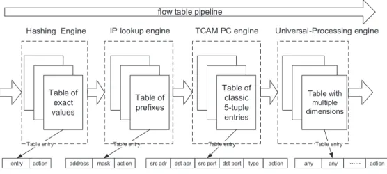
algorithms provide necessary balance between performance and implementation cost. A high-performance flow processing accelerator (framework) is thus proposed to process the pipeline of flow tables. The framework highlighted in Figure 1.2 is composed of four components (engines or modules): a hashing engine for exact-match only tables, an IP lookup engine for prefix-match only tables, a TCAM-based engine for classic quintuple tables, and a universal-processing engine for flow tables featured by multidimensional match with an arbitrary number of fields and any match type.
As shown in Figure 1.2 each framework component adopts a specific approach to process-ing a collection of flow tables.
1. Hashing engine using a highly deterministic hashing scheme [54] for exact-match only ta-bles. We propose two novel collision resolution mechanisms, Double Out hashing and Bidi-rectional Hop Hashing and establish a multiple-segment hash construction to facilitate de-terministic queries. Collision is restricted to only one segment and the length of a probe sequence in each segment is minimized to 1. In addition an important category of false
pos-itive is reduced to 0 due to exact bitmap filters. The use of a unique set of hash functions for filters and hash tables avoids unnecessary computation. The hashing scheme continues our previous work by utilizing hashing and bitmap for not only IP address lookup but also general-purpose high-speed packet processing.
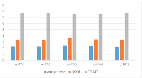
2. IP lookup engine using a hierarchical hashing scheme [52] for prefix-match tables. By tak-ing advantage of bitmap and hashtak-ing techniques effectively used in Tree Bitmap (TBMP) algorithm [14] and Binary hash Searching On prefix Length (BSOL) algorithm [66], our proposed hierarchical hashing scheme significantly improve IP lookup efficiency by remark-ably reducing the number of memory accesses, consuming less memory and enabling fast update.
3. TCAM-based engine characterized by a Divide-and-Conquer Scheme (DCS) [53] for classic quintuple tables. The scheme addresses the range expansion problem which sharply de-grades TCAM storage performance. It allows fast preprocessing, constant time searching, and dynamic incremental update.
Classic quintuple ACL classifiers can be straightforwardly used as flow tables in an Open-Flow switch. TCAM-based solutions benefit from deterministic, constant-time performance. Meanwhile only TCAM-based solution satisfies the high-speed packet-by-packet processing requirement in particular scenarios. [36] introduces such a scenario where a high-performance packet classification engine takes effect when the engine must be placed outside from an OpenFlow switch. From a broader perspective any hardware solution for flow processing is desirable if production cost is bearable.
4. Universal-processing engine using a decomposition approach [55] for flow tables featured by multidimensional match with an arbitrary number of fields and any match type. The
ap-proach performs individual search on each field and conducts a single query in a single hash table. We observe that single field searching is well studied and an efficient LPM method contributes to fast query in individual prefix-match fields without respect to the number of fields in a flow table. Furthermore we address the challenge of efficiently aggregating and combining the results of the single field searches. Our approach scales well to the field number and maintains low latency and incremental update.
Meanwhile these components are not independent. The hashing engine and IP lookup en-gine can be used in the universal-processing enen-gine. Except TCAM-based enen-gine, others can be implemented in either software or hardware, especially in NPU. In the next chapters we introduce each algorithm corresponding to each component in an individual chapter and lay out the frame-work with the overall performance evaluation and analysis. Eventually a conclusion is made in the last chapter.
CHAPTER TWO
HIGHLY DETERMINISTIC HASHING SCHEME USING BITMAP FILTER
2.1 Background
Hash tables are widely used in various network applications for high-speed packet process-ing due toO(1)primitive operations of query, insert and delete [9, 47]. However collisions occur frequently when the table occupancy (load) increases. Newly inserted elements that collide with existing elements are inserted into other buckets thereby leading to an increase in the length of the probe sequence or collision chain, which is followed during the query [31]. Elements at the tail of a long sequence require considerable more probing time than the elements close to the head. Owing to non-determinism caused by long probe sequences the query performance in real-time networking applications is vulnerable to adversarial traffic. In modern hardware devices, multiple threads are coordinated to accelerate hash operations and synchronization is compulsory to keep processing order. While synchronization ensures that requests are tackled in order they arrived, it also reduces overall performance to that of the slowest thread determines. As the number of non-deterministic threads increases, the slowest thread tends to turn much slower and the average query performance degrades tremendously.
Among a variety of hash collision resolution approaches, multiple-segment hashing bal-ances the bucket load by reducing the maximum number of keys in a bucket among all buckets. To avoid probing multiple buckets, on-chip summaries such as Bloom filters link keys in multiple buckets. Several multiple-segment hashing systems proposed in a string of papers [23, 30, 31, 47] remarkably improve deterministic hash operations and achieve good average performance. For instance Peacock hashing [31] limits the length of collision chains in the table segments to a small
constant. Peacock hashing and approaches [30, 47] adopt probabilistic, on-chip filters to reduce off-chip memory accesses and enable deterministic hashing performance. Nevertheless we un-cover critical drawbacks in these systems. Firstly collisions are still allowed in each segment; next the length of the probe sequence is not minimized; and probabilistic Bloom filters only create approximate summary and cannot eliminate an important category of false positive which invites costly off-chip memory accesses in a great number of high-speed networking applications; finally Bloom filters usually employ a distinct set of hash functions from those for table segments. The hash computation overhead for filter query is worthless to hash table access but never trivial when under heavy network traffic.
Bloom filters used in previous multiple-segment hashing systems do not discriminate be-tween two categories of false positive. The first category occurs when any request must match some element in one segment but the match result is wrongly reported in the other segment(s). In other words only when the element is exactly matched in the unique, correct segment, the first category of false positive never happens. The second category occurs when a request should not match any element but the matching result is wrongly reported in one or more segments. The first category is of great significance to high-speed network applications which do not need to handle the second category. For example, IP address lookup forwards packets using routing tables. In a routing table a rule with lowest priority usually matches any packet which does not match others. For another instance, rule sets used in packet classification algorithms usually contain a rule which matches any packet. Or there is always a miss-flow entry in an OpenFlow flow table with the same functionality. A Bloom filter can only reduce but never eliminate the first category. In a high-speed network device which processes millions of packets every second, tens of thousands of packets are mismatched even with a 1% false positive in a multiple-segment hashing system using Bloom filters, leading to costly off-chip memory access. The situation becomes worse as the volume of
network traffic increases.
In the dissertation we establish a multiple-segment hashing system using Double Out hash-ing (DOhashing) and Bidirectional Hop hashing (BHhashing). Our hashing construction, called the hierarchy, consists of the number ofnhash segments (tables) ordered by insert sequence. Each hash table acts as a collision buffer for the tables with higher order and uses a distinct hash func-tion to reduce collision probability. Collision is only allowed in the lowest-order table adopting BHhashing. Other tables useDOhashing to avoid collision with the aid of on-chip bitmap filters. Our scheme outperforms previous multiple-segment hashing schemes by:
• promoting deterministic query performance to facilitate network processing by restricting collision to only one hash table and minimizing the probe sequence to only 1 in each hash table;
• eliminating a significant category of false positive using innovative on-chip bitmap filters;
• avoiding unnecessary hash function computation for on-chip filter queries.
2.2 Related Work
A number of related work discussed various perspectives to improve hash performance for high-speed network applications. The importance of determinism for hardware performance was studied in [12, 31]. Demetriades et al. [12] resolves collision and guarantees deterministic IP lookup by dynamically migrating IP prefixes. Researchers [47, 59] attempt to ensure that a single bucket reference is used for each table lookup with high probability. Simple hash functions [28] are suggested for essentially the same performance as a truly random hash function which causes heavy computation overhead. The Hash Index Table [24] proposes a novel on-chip filter. Huang et al. [23]
reduce on-chip memory consumption by storing hashed bucket addresses into an intermediate index table but incur space overhead and delays due to indirect access. Our scheme is influenced by these work and will show determinism can be improved by better resolving collisions in each hash table. Our scheme uses simple hash functions and on-chip bitmap filters for exact summary and quick query.
Some researchers [9,12,25,27] argue multiple-segment hashing is among the best solutions to resolve collision. Our primary starting points are Fast Hash Table (FHT) [47] which summarizes the locations of items in a hash table that uses multiple hash functions, and Peacock hashing [31] that greatly reduces on-chip memory consumption compared to FHT while keeping determinism by limiting the length of the probe sequence in each table to a small constant. Both achieve a deterministic performance by providing multiple table locations before inserting any new element. To avoid multiple off-chip memory accesses they use probabilistic Bloom filters and hence enable deterministic hashing performance. We will show our scheme further improves determinism and eliminates drawbacks of Bloom filters.
2.3 DOhashing andBHhashing
2.3.1 DOhashing
We inventDOhashing for highly deterministic query. A Double Out hash table (DOtable)
Ti(1≤i≤n−1) is an array of buckets. Given an elementEits indexidx inTiis computed using
hi(E),Ti’s associated hash function. A bucket contains at most one element. Ti is associated with three auxiliary structures: a main bitmap filterBi, a collision table ColTi and a collision bitmap filter ColBi. Bi maintains an exact summary of Ti buckets and each Bi bit is associated with a specific Ti bucket. It is set if the bucket contains an element, or clear otherwise. ColTi keeps
Empty
Collision Occupied
D I
D
Bit clear in both Bi and ColBi Bi bit set and ColBi bit clear
Bi bit clear and ColBi bit set I D State 1 State 2 State 3 I
Figure 2.1: Three Bucket States
references to all the collided elements in Ti. A reference (j,index) to E indicatesE’s residing table Tj and corresponding index. A ColTi bucket is associated with a specific Ti bucket and keeps a linked list of references to collided elements in the Ti bucket. ColBi maintains an exact summary ofColTibuckets and eachColBibit is associated with a specificColTibucket. It is set if the list in the bucket is not empty, or clear otherwise.
A DO table Ti and its auxiliary structures have the same dimension. Furthermore a Ti bucket’s index is the same position to access its associatedBi bit,ColBibit, andColTibucket. As the only hash function forTi and its auxiliary structures,hi is used for index computation.
A bucket state reveals how primitive operations are performed in aDO table. Figure 2.1 demonstrates the state transfer among State 1 (Empty), State 2 (Occupied), and State 3 (Collision). A circle symbolizes a state and a directed arrow expresses a single primitive operation, e.g.Dfor a delete andIfor an insert attempt. A bucket state is marked by aBibit and aColBibit collectively, e.g. State 2 byBi bit set andColBibit clear.
State 1 stands for an empty bucket. When an element is inserted, State 1 is transferred to State 2. State 2 implies that an element resides in the bucket. After deleting it State 2 is transferred to State 1. When another element is indexed to a bucket in State 2, the collision occurs and State 2 is transferred to State 3. The existing element is deleted and both elements try the next lower-order
hash table. A State 3 bucket remains empty and rejects the insert attempt of any new element which has to try the next table. Thus no state transfer occurs in a State 3 bucket for any insert attempt. A delete in a State 3 bucket causes two outcomes. The first outcome does not incur state transfer but the second one does. We will illustrate them later. ADOtable disallows collision and restricts the length of a probe sequence to only 1.
The consequence of inserting an elementEtoTj relies on current bucket state.
• State 1: no collision and inserted.
• State 2: encounter collision. Remove the existing element and try both elements inTj+1.
• State 3: still collision and tryE inTj+1.
Algorithm 1 states the insert procedure. Re-balancing will be discussed in the delete pro-cedure. All collided elements which fail to be inserted to theDOtableTn−1 will tryTn. The insert procedure reveals that an element must reside in only one hash table. OnceE is inserted intoTi, its reference is added into eachColTj(1≤ j ≤ i−1) and theColTjbucket’s index is computed usinghj(E).
Figure 2.2 exhibits a simple insert and delete example using twoDOtables consisting of 8 and 6 buckets respectively. In Figure 2.2(a)T1containsE1 inb3 (index as subscript). T2is empty and not shown. New elementE2 collides withE1 inb3. Figure 2.2(b) demonstrates the collision outcome. ColT2andColB2 are not shown. SupposeE1 andE2 are inserted into different buckets
b5 andb0 inT2. So listL3 ofColT1 contains their references, (2,5)and(2,0)respectively. B1’s corresponding bit is clear andColB1’s bit in the same position is set whileB2’s corresponding bits are set.
Elements inT1can be deleted without involving any collision table. However if an element
Algorithm 1Insert Algorithm forDOTable
FuncDoubleOutInsert(E,i){i: table number ofTi} intidx =hi(E);{calculate index}
Bucketb=Ti.getBucket(idx);
ifbin State 1then Ti.insert(idx,E);
for allj from 1 toi−1 do
intnewIdx =hj(E);{recalculate index} ColTj.insert(newIdx,i,idx);{insert reference}
else
ifbin State 2then
Ec=Ti.remove(idx);{Ec: existing element} FuncDoubleOutInsert(Ec,i+ 1);{tryEcinTi+1} FuncDoubleOutInsert(E,i+ 1);{tryEinTi+1}
else
FuncDoubleOutInsert(E,i+ 1);{bin State 3}
T1 ColT1
T2
(c) after deleting E1, L3of ColT1contains only E2reference
T1 ColT1 (d) move E2to b3of T1 B1 B1 B2 b0 b1 b2 b3 b4 b5 b6 b7 1 0 0 0 0 0 0 0 1 0 0 0 0 0 0 0 0 1 0 0 0 0 ColB1 0 0 0 1 0 0 0 0 ColB1 0 0 0 1 0 0 0 0 T1 ColT1 E2
(a) try E2in T1and it collides with E1in b3 0 0 0 0 0 0 0 0 T1 ColT1 1 0 0 0 0 1 T2 (b) insert E1into b5of T2, E2in b6of T2 B1 B1 B2 2 , 5 3 , 2 0 0 0 0 0 0 0 0 b0 b1 b2 E1 b4 b5 b6 b7 b0 b1 b2 b3 b4 b5 b6 b7 ColB1 0 0 0 1 0 0 0 0 ColB1 E2 b1 b2 b3 b4 E1 b0 b1 b2 b3 b4 b5 b6 b7 b0 b1 b2 L3 b4 b5 b6 b7 2 , 0 b0 b1 b2 L3 b4 b5 b6 b7 E2 b1 b2 b3 b4 b5 b0 b1 b2 E2 b4 b5 b6 b7 0 0 0 1 0 0 0 0 b0 b1 b2 b3 b4 b5 b6 b7
tables from ColT1 to ColTj−1 and each list resides in the bucket with index of hj(E). As we discussed in Figure 2.1, two outcomes happen after a delete in a State 3 bucket. After removingE’s reference if any list contains at least two references, this is the first outcome and no state transfer occurs in any bucket. However if any list contains only one reference, the second outcome happens as shown in Figure 2.2(c) and (d). Return to the example and now deleteE1. Figure 2.2(c) displays its reference in L3 ofColT1 is also removed. SinceL3 ofColT1 contains only one reference of
E2, no collision exists inb3ofT1any more and under this circumstanceE2should be moved back. Figure 2.2(d) shows the result of movingE2 fromb0 ofT2 to b3 ofT1. Its reference is removed from ColT1. T2 is empty and not shown. B1’s associated bit with b3 of T1 is set and ColB1’s associated bit withL3ofColT1is cleared. The delete in one bucket, e.g. b5 ofT2, causes the state transfer at another bucket, e.g. b3 ofT1, from State 3 to State 2 in Figure 2.1.
Algorithm 2 states the delete procedure. Given an element E to be deleted, its current residing tableTiand its bucket indexb, the delete procedure proceeds as illustrated in Figure 2.2(c) and (d) if the collision list with the only reference after the deletion is detected. E’s reference in all its previous collision tables should be removed. Once it is removed, the detection of one-reference list in current collision table is performed. If current list contains only one reference, that indicates no collision for this reference. New insertion should be conducted. Therefore a simple deletion may lead to a great number of chaining reaction for insertion and deletion. It is not reasonable for frequent update.
Re-balancing is defined as a process to achieve load balance among hash tables by moving elements from low-order tables to high-order tables. Re-balancing takes place whenever a delete operation gives rise to a one-reference collision list which leads to more deletions and insertions. Through re-balancing an element is moved to the first hash table where it has no collision, e.g. moving E2 from T2 to T1 in Figure 2.2(d). Re-balancing also takes effect when one-reference
Algorithm 2Delete Algorithm forDOTable
FuncDoubleOutDelete(E,i,b){E: element to be deleted;i: EinTi;b: bucket index}
Ti.remove(b);{delete this element}
Bi.clearBit(b);{clear correspondingBi bit}
for allj from 1 toi−1 do
intnb=hj(E);{calculate new index} ColTj.delete(nb,i,b);{deleteE’s reference}
ifColTj[b].size= 1then
intni=getT N o(ColTj[b](0));{the only element inTni}
intnIndex=getIndex(ColTj[b](0));{this element’s index inTni}
nE =getElem(ni, nIndex);{retrieve this element} ColTj.delete(j,ni,nIndex);{delete this reference} FuncDoubleOutInsert(nE,ni);{insertnE inTni}
list is generated by discarding one element due to an insert in a State 2 bucket. Re-balancing is of extraordinary significance to maintain global load balance in the hash tables. Without it State 3 buckets in high-order tables cannot preserve new elements, leading to ever-increasing load in low-order tables and eventually high discard rate inTn.
2.3.2 BHhashing
We designBH hashing forTn (theBHtable) which allows one collision for each bucket. The first collided element in a bucket may be inserted in a backup bucket through bidirectional searching in a neighborhood area. The backup bucket is called next-hop and current bucket is called previous-hop. Their relation is expressed using a bitmap. An element is discarded if it is indexed to a bucket with next-hop or the bidirectional searching returns a non-empty bucket. The discard rate is the percentage of elements dropped inTn. IfTncontains more next-hops the discard rate increases. If an elementE in a bucket is deleted, the element in the bucket’s next-hop needs to be moved to the bucket. This substantially improvesTnload and diminishes the discard rate. In additionE’s references in all collision tables are removed.
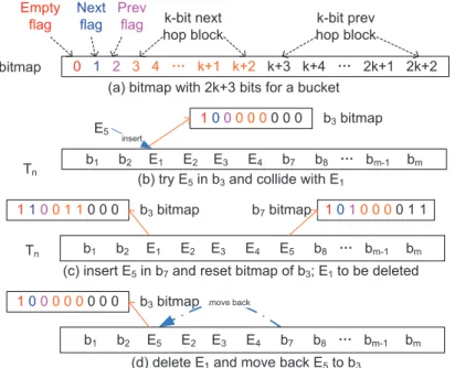
A binary bitmap is associated with a bucket to encode collision information. We choose the value ofk, a tunable parameter, to vary the bidirectional searching distance. Larger k values increase the opportunity for an element to find its next-hop in the bidirectional searching and hence reduce the discard rate in general. Figure 2.3(a) depicts a bitmap format with 2k+3 bits. From left the first bit indicates whether the bucket is empty. The second bit indicates whether the bucket has a next-hop. If it is set, the k-bit next hop block (index from 3 tok+2) encodes the relative distance to the next-hop in binary. The third bit indicates whether the bucket has prev-hop. If it is set, thek-bit prev-hop block (index fromk+3 to2k+2) encodes the relative distance to prev-hop. In practice the second bit and k-bit next-hop block (or the third bit and k-bit prev-hop block) act as the next pointer (or the previous pointer) in a double linked list.
The neighborhood of a bucket bp covers 2k buckets, forwardly from bp+1 to bp+2k−1 and
backwardly frombp−1tobp−2k−1. The bidirectional searching starts forwardly and then backwardly.
As soon as an empty bucket is found, the bidirectional searching terminates and returns the bucket. If no empty bucket is found, discard the element.
Figure 2.3 displays an example of insert and delete in theBH table. Assume k = 3. Tn contains four elements. b3 (index as subscript) containsE1 and has no next hop. The first bit ofb3 bitmap is set. b4, b5 andb6 contain E2, E3 and E4 respectively and their bitmaps are not shown. In Figure 2.3(b)E5is indexed tob3 and collides withE1. The bidirectional searching begins from
b4 and returnsb7 to whichE2 is inserted since buckets fromb4 tob6 are not empty. Figure 2.3(c) describes the connection betweenb3 andb7. The second bit inb3 bitmap is set for next-hop and
k-bit next-hop block encodes the distance 4 (011in binary). Likewise the first and third bits inb7 bitmap are set for non-empty and prev-hop indication, andk-bit prev-hop block encodes the same distance. In Figure 2.3(d)E1 is deleted. E5 inb3’s next hopb7is moved back tob3. Sob7is empty and its bitmap is not shown. Eventually only the first bit inb3bitmap is set to representE5.
0 1 2 3 4 Ă k+1 k+2 k+3 k+4 Ă 2k+1 2k+2 bitmap Empty flag Next flag Prev
flag k-bit next hop block
k-bit prev hop block
(a) bitmap with 2k+3 bits for a bucket
b1 b2 E1 E2 E3 E4 b7 b8 Ă bm-1 bm
Tn
insert
E5
(b) try E5in b3and collide with E1
1000 0 0 0 0 0 b3bitmap
b1 b2 E1 E2 E3 E4 E5 b8 Ă bm-1 bm
Tn
(c) insert E5in b7and reset bitmap of b3; E1to be deleted
1100 1 1 0 0 0 b3bitmap b7bitmap 1010 0 0 0 1 1
(d) delete E1and move back E5to b3
move back
b1 b2 E5 E2 E3 E4 b7 b8 Ă bm-1 bm
1000 0 0 0 0 0 b3bitmap
Figure 2.3: Bitmap Format, Insert and Delete in theBHTable
By choosing a reasonablek value, a cache line can contain an element and its next-hop. In consequence only one memory access is sufficient to query an element. This eradicates the drawback of cuckoo hashing [38] or linear hashing, i.e. the need to access sequences of unrelated locations on different cache lines.
2.4 Hierarchy Design
From what we have discussed above, multiple-segment hashing balances the bucket load by reducing the maximum number of keys in a bucket among all buckets. The use of on-chip summaries further reduces the number of probes in multiple buckets. Several multiple-segment hashing systems such as Peacock hashing and FHT have fairly good performance. Thus our pro-posed scheme is based on similar hierarchical structure with multiple hash segments. In our scheme DOhashing andBHhashing work collaboratively. All the hash tables except the last one employ
b0 b1 b2 b3 b4 b5 b6 ĂĂ 0 0 0 0 0 0 0 ĂĂ ColT1 ColB1 T1 B1 b0 b1 b2 b3 b4 b5 b6 ĂĂ 0 0 0 0 0 0 0 ĂĂ b0 b1 b2 b3 b4 ĂĂ 0 0 0 0 0 ĂĂ ColT2 ColB2 T2 B2 b0 b1 ĂĂ 0 0 ĂĂ ColTn-1 ColBn-1 Tn-1 Bn-1 b0 b1 b2 b3 b4 ĂĂ 0 0 0 0 0 ĂĂ b0 b1 ĂĂ 0 0 ĂĂ
Ă
Ă
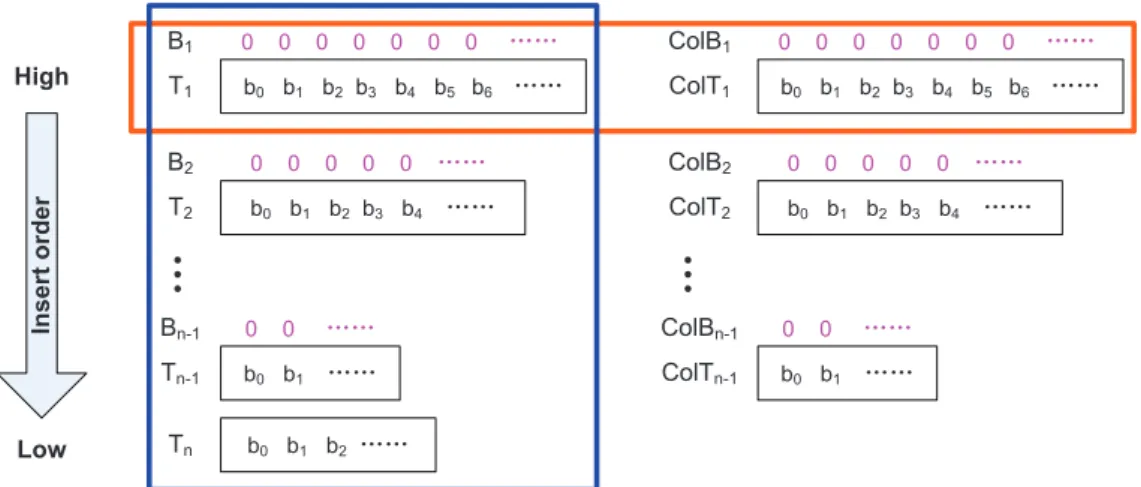
b0 b1 b2 ĂĂ Tn High Low In s e rt o rd e rFigure 2.4: Hash Table Hierarchy
DOhashing for the benefit of fast query using on-chip filters. Collision is disallowed in eachDO table, and the length of a probe sequence is limited to only 1 accordingly. The BH table adopts BH hashing, stores the collided elements in all theDO tables, and allows one collision for each bucket. Only one memory access is needed in theBHtable to look up two associated elements in a cache line.
Figure 2.4 depicts the hierarchy framework. The vertical block highlightsnnumber of hash tables. The insert order is the table sequence to insert an element andT1 is always the first choice to try an elementE. IfE collides inT1, tryT2. Continue to tryE in each lower-order table along the insert order until it is either inserted into a table without collision or discarded if it fails to be inserted in Tn. Thus each hash table except T1 acts as a collision buffer for higher-order tables. The horizontal block encircles T1 and its three auxiliary structures, also in everyDO table. Our scheme follows two fundamental principles.
1. Keep as few elements as possible inTn.
Principle 1 enablesDOtables to contain the majority of elements for the sake of fast query using on-chip filters. According to Principle 2 an element is inserted toTj(j >1) only if it collides in all the higher-order tables, i.e. fromT1toTj−1. A delete of an elementEfromTj (j >1) leads to removal ofE’s all references in the collision tables fromColT1toColTj−1. Principle 2 results in element movement due to re-balancing under one-reference list circumstance.
In terms of the framework and principles we need to determine three essential aspects in the hierarchy. Firstly is there an optimal load for a DO table and what is relation between load factor and discard rate in the BH table? Secondly what is an ideal number of hash tables in the hierarchy and how to assign table dimension given an input set? Finally how to query an element using filters and tables? Our purpose is to achieve balance between memory consumption, discard rate and query efficiency. In the remaining dissertationci denote the dimension of a hash table. m andmirepresent the numbers of elements in all hash tables andTi (theithtable) respectively.
2.4.1 Load Analysis
An element is discarded if indexed to aTnbucket with next-hop or the bidirectional search-ing returns a non-empty bucket. Therefore largerTnload gives rise to more next-hops and a larger discard rate. We discover that at 38% load the discard rate is about 1% and all the discarded ele-ments are only attribute to next-hop collision. The bidirectional searching always returning empty buckets even with a fairly smallkvalue, e.g. 2.
FormallySwrepresents the number of buckets in aDOtableTiunder Statew(1≤w≤3). So
3
∑
w=1
Sk = ci whereinci is Ti dimension. Suppose an element has an equal probability to be indexed in any bucket. Equation (2.1) counts the number of State 2 buckets inTi where ri is the
number of elements to be inserted. S2(ri) =ri× ( 1− 1 ci )ri−1 (2.1)
ρiis defined as the ratio of input elements to the number ofTibuckets and calculated by rci
i.
Equation (2.1) derives Equation (2.2) wheref(ρi), a function ofρi andci, signifiesTi’s load. The optimal value off(ρi)is proven in Lemma 1.
f(ρi) =ρi× ( 1− 1 ci )ρi×ci−1 (2.2)
Lemma 1.ρB =e−1atρi = 1whenci → ∞. eis base of natural logarithm.
Proof. To reach the peak value off(ρi), df(ρdρii) = 0. Equation (2.3) is derived from Equa-tion (2.2). (1− 1 ci ) ρi×ci−1 +ci×ρi×(1− 1 ci ) ρi×ci−1 ×ln(1− 1 ci ) = 0 (2.3)
Equation (2.4) is thus obtained from Equation (2.3).
ρi = − 1 ci×ln ( 1− c1 i ) (2.4) Now limci→∞ ( 1− c1 i )ci = e−1 when c
i → ∞and ρi = 1. Eventuallyf(ρi) reaches its peak value atρB in Equation (2.5) whereρB is defined as theρi value (100%) leading to optimal load. In conclusion when the dimension of a DO table equals the input size, its optimal load is
e−1,≈36.79%. f(1) = lim ci→∞ ( 1− 1 ci )ci−1 =e−1 (2.5)
2.4.2 Dimension Assignment
On basis of Equation (2.5) we propose a hierarchy to obtain optimal load in allDOtables. Given an input set with size m, c1 is set to be mto meet ρB = 1 andm1 = c1 ×ρB. SoT1 has a theoretical optimal load. The number of collided elements in T1 is c1 ×(1−ρB), used as the input toT2. Thereforec2 is set to bec1×(1−ρB)andm2 =c2×ρB. The remaining elements are used as the input toT3. Repeat the dimension assignment strategy until in some point assign the remaining elements tocn. Equation (2.6) summarizes the strategy.
ci =m×(1−ρB)i−1;mi =m×(1−ρB)i−1×ρB (2.6)
According to Principle 1 we use a tunable parameterβ to determine the upbound per-centage of elements assigned toTnand the parameter directly determines the total number of hash tables. If ci−mi
m < β we set cn. Recall that discard rate is around 1% at 38% Tn load. Thus
cn= cn−10.38−mn−1 and the number of buckets in all the hash tables is approximatelym×e. Table 2.1: 8-table Hierarchy
ci c1 c2 c3 c4 c5 c6 c7 c8 c= 8 ∑ i=1 ci Size 100000 63210 39954 25254 15962 10088 6376 10605 271449
Table 2.1 shows an 8-table hierarchy givenm = 100000,β = 5% andρB = 36.79%. c1 is exactlym. m1 =m×ρB or 36790. Usec1 −m1 as input toT2 andc2 = 63210. Continue until
c7−m7
m < β andc8 = c7−m7
0.38 , or 10954. Ifβ increases, the number of hash tables decreases. For example under 7% value ofβ, the number of hash tables is 7 and the last tableT7has a dimension
c7 of 17331. In case thatβ = 7%, the number is 6 withc6 = 27421. Though the number of hash tables varies along with differentβ, the optimal load is maintained in each DO and the hashing
performance is thus not affected. For the purpose of incremental update a smaller constant thanρB is more practical for real implementation because higherρBmore likely leads to larger drop rate if a more restricted drop rate is imposed.
2.4.3 Query
To query an elementE, each index idxi (1 ≤ i ≤ n−1) for aDOtableTi is calculated usinghi(E). Firstly all the bits at idxi position of main and collision filters are inspected in on-chip memory. Next a hash table access is taken in main memory only when the following two bit patterns are matched.
1. No positive response from main filters. EachBi bit is clear and eachColBibit is set. 2. At least one positive response from main filters. SupposeTj is the highest-order DOtable
whose associatedBj contributes a positive response. So eachBl (1≤l ≤j−1) bit is clear and theBj bit is set while eachColBlbit is set and theColBj bit is clear.
If pattern 1 fires, access a correspondingTnbucket and its next-hop if necessary. If pattern 2 fires, accessTj bucket inidxj. In case of other bit patterns no hash table is accessed asE does not match any element.
Algorithm 3 describes the query procedure. The first inspection is performed in both bitmaps. If two valid patterns are discovered, a memory access is conducted to either Tj or Tn. Otherwise, the query packet does not match any input element as its corresponding bit pattern is regarded as invalid. Function query() and queryN() make hash access intoTj andTngiven a target request and return the corresponding action.
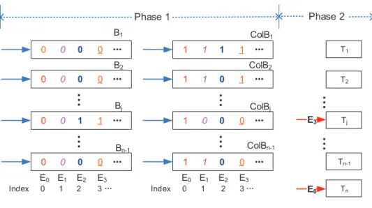
Figure 2.5 elaborates how to query four elements, E0 to E3, according to Algorithm 3. Suppose their indexes are 0, 1, 2 and 3 respectively in all the hash tables. Actually it is impossible
Algorithm 3Query Algorithm FuncQuery(E){E: given request}
action= empty;{the action}
bitarrayarrB= empty;{bit array for main bitmap} bitarrayarrColB = empty;{bit array for collision bitmap}
for allj from 1 ton−1 do
arrB[j] =Bj.getBit(E);
arrColB[j] =ColBj.getBit(E);
ifarrBandarrColB in pattern 1then action= query(Tn);{accessTn}
else
ifarrB andarrColB in pattern 2then action= query(Tj);{accessTj}
else
action= none;{invalid request} returnaction
for an element to have the same index in each hash table. We simply make the assumption for expression convenience in the example. Firstly all the filters are inspected. ForE0, the bits at index 0 are all clear in the main filters and all set in the collision filters. Therefore pattern 1 matches. For
E1, pattern 1 does not match since the bit at index 1 ofColBj is not clear. ForE2, pattern 2 does not match since the bit at index 2 ofColB1 is not clear. For E3, each Bl (1 ≤ l ≤ j −1) bit is clear and theBj bit is set while each ColBlbit is set and theColBj bit is clear. Therefore pattern 2 matches. Consequently E1 and E2 match no element. Next Tn is accessed to queryE0 using
hn(E0)andTj is accessed forE3.
Throughout query procedureDO hashing guarantees no collision in the majority of hash tables and BH hashing ensures a single cache-line access. Query is thus performed in a highly deterministic manner because only one hash access is needed for any query and the length of probe sequence in each table is minimized to 1. Additionally the first category of false positive is reduced to 0 and unnecessary hash function computation is avoided for filter queries. Actually
0 0 0 0 Ă Tn
Ă
0 0 0 0 Ă 0 0 1 1 ĂĂ
0 0 0 0 Ă 1 1 1 1 ĂĂ
1 1 0 1 Ă 1 0 0 0 ĂĂ
1 1 0 0 Ă T1 T2 Tj Tn-1Ă
Ă
E0 B1 B2 Bj Bn-1 ColB1 ColB2 ColBj ColBn-1 Phase 1 Phase 2 Index 0 1 2 3 Ă Index 0 1 2 3 Ă E3 E0 E1 E2 E3 E0 E1 E2 E3Figure 2.5: Query Example
queries in filters are independent and can be paralleled. Our scheme is highly qualified for hardware implementation accordingly.
2.5 Simulation
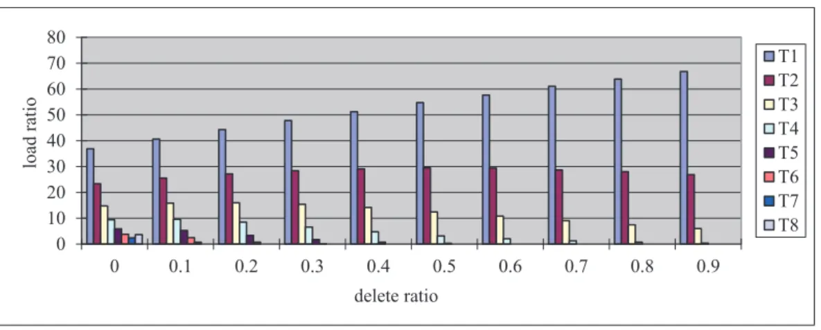
The simulation is performed in a commodity computer to evaluate several significant per-formance metrics including re-balancing influence, update efficiency and memory usage. The ad-vantages and disadad-vantages of the use of on-chip filters in our scheme are compared with FHT and Peacock hashing. All the experiments in the simulation are conducted upon the proposed 8-table hierarchy using input sets from 5 groups of real IP routing tables [2]. Each input set has 100,000 elements randomly chosen from a routing table after eliminating duplication and each experiment is repeated 10000 times per input set when we generate the matching packets against each input set. Through experiments we discover that the averageDOtable load is nearly optimal, consistent with theoretical analysis. In addition the first category of false positive is exactly 0. The bit pattern of each queried element exactly matches either pattern 1 or pattern 2.
0 10 20 30 40 50 60 70 80 0 0.1 0.2 0.3 0.4 0.5 0.6 0.7 0.8 0.9 loa d r a ti o delete ratio T1 T2 T3 T4 T5 T6 T7 T8
Figure 2.6: Rebalancing Consequence
We choose two groups of hash functions. The first group only uses CRC32 with differ-ent feed length for each hash table. The second group consists of eight various message digest functions such as SHA-256. The experimental results using the two groups show that there is no difference in two crucial performance metrics, the average lengths of the collision lists and the global distribution of elements in all the hash tables. Consequently the hash function choice is independent from the hash performance.
2.5.1 Re-balance Influence
We observe the re-balancing influence through the distribution of remaining elements after deleting a percentage of elements, randomly chosen from all the hash tables. The percentage varies from 0% to 90%. Distribution ratio is formulated as mi
m (1 ≤ i ≤ n) where mi is the number of elements in a table andmis the number in all the tables after re-balancing.
Figure 2.6 accounts for the re-balancing influence. Vertical axis and horizontal axis repre-sent the distribution ratio and the percentage of deleted elements. Each column points out a table’s distribution ratio. As the delete percentage increases, we observe three phenomena. Firstly the
dis-tribution ratios of low-order tables becomes 0 as a result of element movement towards high-order tables. For example only a few elements remain inT8after 10% percentage deletes. In tables from
T4 toT8distribution ratios decrease monotonically. SecondlyT1’s distribution ratio monotonically increases. Thirdly the distribution ratios ofT2 andT3 increase and then decrease. For example at delete percentages less than 50% elements moved from lower-order tables are more than elements deleted out of T2. ThusT2’s distribution ratio increases. Otherwise the ratio decreases as lower-order tables are almost empty and the outgoing elements overpasses the incoming elements inT2. These phenomena explain how re-balancing facilitates global load balance by moving elements to high-order tables. Re-balancing caused by a simple deletion is finished whenever all colliding elements find their suitable buckets.
2.5.2 Update Efficiency
Update involves bitmap filters, hash tables and collision tables. An insert attempt in aDO table may cause collision and hence an existing element is deleted from the table. The chaining reaction due to one insert may be propagated to lower-order hash tables. In the worst scenario
O(2n−1) elements may be deleted owing to an insert and more deletes occur in collision tables. Nevertheless the average update performance is much better in the simulation. Averagely only one element is deleted from the hash tables owing to an insert. Meanwhile averagely 5 insert and delete operations occur in collision tables per hash table insert. On the other hand a delete may involve element movement to high-order tables due to re-balancing. Though the worst delete case is difficult to analyze, average delete efficiency can be evaluated by the average number of moved elements per delete. Averagely 2 elements per delete are moved and 4 insert and delete operations occur in collision tables per hash table delete.
2 bits, one in a main filter and the other in a collision filter, represent an element while 10 bits represent an element in Bloom filters used by FHT and Peacock hashing. Thus a limited number of off-chip and extremely few on-chip memory accesses per update operation justifies the capability of incremental update in our scheme.
2.5.3 Memory Evaluation and Filter Comparison
A reference in a collision table occupies a few bytes in real data structures. By comparison a hash table element usually consists of dozens, or even hundreds, of variant bytes and hence hash tables consume the majority of main memory. In the proposed hierarchy the total amount of buckets is approximatelym×ewheremis the input size andeis base of natural logarithm. The main memory consumption in our scheme is moderate concerning less than three folds of input size, reasonable for deployment in network processors which nowadays are equipped with plenty of main memory.
Table 2.2: Comparison Results
Scheme 1stFP On-chip Mem Usage Filter Hash Function
FHT 1% 10×m separate
Peacock 1% m separate
Ours 0 2e×m identical
Table 2.2 compares our scheme with Peacock hashing [31] and FHT [47] in three on-chip filter metrics. 1stFP represents the first category of false positive, 0 in our scheme. The other two schemes use Bloom filter with nearly 1% false positive rate. There is no false negative in all schemes. Concerning the on-chip memory usage, to restrict the false positive to 1% a 10-bit, on-chip memory is used for each element and hence FHT uses10×mbits whereinmis the input size. Peacock hashing utilizesm bits because about 10% of elements are represented using filter
bits. In our scheme all filters use a total of 2e×m bits, e.g. less than 1MByte on-chip memory given an input size of one million. Our scheme employs a unique set of hash functions for all the filters and tables. In the other schemes the set of Bloom-filter hash functions varies from the set of hash functions for hash tables. Consequently our scheme eliminates the double hash computation overhead. Furthermore bitmap filter update is more efficient in our scheme as discussed before. In a high-speed network device, e.g. a core router, which processes billions of packets per second, millions of packets are mismatched even with a 1% false positive, leading to considerable off-chip memory access. As well the extra computational overhead for separate filter hash function can never be considered trivial. The situation becomes even worse as the volume of network traffic rapidly increases.
Though our scheme consumes more on-chip memory than Peacock hashing, the novel de-sign of exact summary using bitmap filters eliminates the first category of false positive and avoids unnecessary hash computation for filter query. The trade-off is particularly valuable for numerous high-speed network applications to accelerate packet processing. On-chip memory consumption is easily satisfied by modern hardware devices such as network processors. Despite false positives in the second category, only one memory access is needed in our scheme and hence high deterministic performance is maintained.
2.6 Summary
By means of novel collision resolution mechanisms high deterministic performance is achieved in our scheme. An important category of false positive is reduced to 0 and unnecessary computation for filter query is avoided. Through mathematical reasoning we propose a hierarchy with optimal load in each hash table and low discard rate. Simulation results adequately justify the efficiency of re-balancing and incremental update. The comparison to other schemes distinguishes
effective use of the exact-summary, bitmap filter in our scheme. In conclusion our scheme is highly qualified for hardware implementation to boost network processing. Future work intends to focus on rehashing to accommodate more frequent updates and multiple next hops in aBHtable bucket.
CHAPTER THREE
HIERARCHICAL HASHING SCHEME TO ACCELERATE LONGEST PREFIX MATCHING
3.1 Introduction to IP address lookup
Longest prefix match (LPM) techniques use similar packet classification algorithms and data structures such as hashing, tree, and trie to reduce computational complexity. They can be classified into two categories as well: software-based and CAM-based (hardware). Likewise, both are crucial for high-performance table lookup of exact-match or prefix-match types of flow tables in OpenFlow switches.
Hardware solutions, e.g. TCAM, can search contents in parallel to achieve constant time complexity. However, they still suffer from limited memory and high power consumption. Thus, only limited entries are suitable to perform in TCAM. By contrary software schemes benefit from low cost and flexibility.
• Trie-based algorithms. The original one-bit trie algorithm organizes the prefixes with the bits of prefixes to direct the branching [64]. However, since its worst-case memory access is so high that many other techniques have been integrated to reduce the height of trie (like Patricia, LC trie [37], LPFST [67] etc), but the usage of these techniques often leads to hard updating or memory expansion. TBMP [14] proposes a compressed trie data structures that have small memory requirements, fast lookup and update times by using two bitmaps per trie node. It keeps the trie node sizes small by separating out the next hop information into a separate results node that is accessed lazily at the end of the search and thus do the complete processing in one memory access per trie node. Although TBMP achieves good
performance, it still suffers from searching efficiency and performance degradation resulting from variable child-node storage.
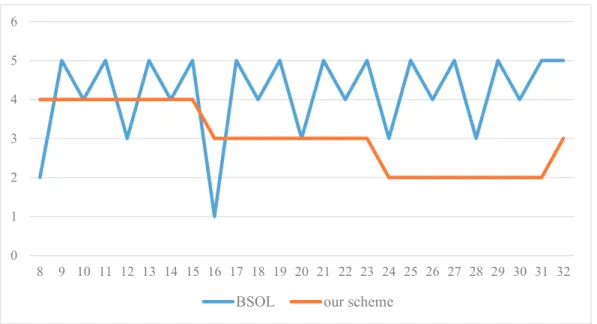
• Hash-based algorithms. Hash has an outstanding feature ofO(1) run-time, and many net-work processors have build-in hash units. Besides, lots of research net-works have proposed many hash approaches for IP lookup. In particular, the BSOL algorithm [66], which has the best theoretical performance of any sequential algorithm for the best-prefix matching problem, uses hash tables. The algorithm described in [35], uses parallel search of on-chip Bloom filters to identify which of a number of off-chip hash tables must be searched to find the best matching prefix for a given packet. In [66], prefixes are grouped according to their lengths and stored in a set of hash tables. A binary search on these tables is performed to find the matching prefixes of the destination IP address. Each search step probes a corresponding hash table to find a match. By storing extra information along with the member prefixes in hash tables, a match in a given table implies that the longest matching prefix is at least as long as the size of prefixes in the table, whereas a failure to match implies the longest matching prefix is shorter.
Only [7] prototypes layer-3 IP routing based on OpenFlow flow tables, actually routing tables. Our proposed work deals with flow tables not only in IP lookup with one dimensional prefix match or exact match using hierarchical hashing, but also multiple dimensional flow processing including packet classification, which will be introduced later.
3.2 Background
The rapid growing of Internet traffic demands routers to perform high-speed packet for-warding. Drastic increases in volume of traffic result in large routing tables and thus require faster
lookup. As a consequence Longest Prefix Matching (LPM) for IP Address lookup becomes a chal-lenging task, often the bottleneck in routers and efficient schemes to perform LPM in high-speed routers are needed.
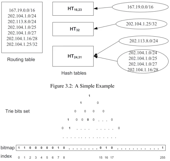
A routing table in a router stores variable-length IP address prefixes and corresponding out-going ports (next-hop). A prefix is an IP destination address with mask, such as 2001:0cb0:c202::/48 in IPv6 or 202.104.1.0/24 in IPv4. The mask is also called the prefix length. Two prefixes may have the same IP address and distinct masks. When a packet arrives, a router gets the destination address in its header, finds the prefix by means of LPM in the routing table, and forwards the packet according to the corresponding next-hop. Table 3.1 displays a simple IPv4 routing table with 7 entries.
Table 3.1: An IPv4 Routing Table
IP Address Mask Next-hop (Port)
167.19.0.0 16 2 202.104.1.0 24 1 202.113.8.0 24 3 202.104.1.0 25 4 202.104.1.0 27 2 202.104.1.16 28 3 202.104.1.25 32 1
Several metrics are essential to evaluate the performance of IP lookup algorithms. Lookup time or searching speed is the paramount metric, essentially determined by the number of memory accesses (worst and average) as memory access is the most time-consuming step in the lookup procedure [65]. Memory consumption is also important for routing tables can grow quite large and may contain as many as four hundred thousand prefix entries. In addition, update complexity, efficiency, scalability and ease of implementation are also important for actual deployment as well.