Identification of Radar Signals Based on Time-Frequency Agility using Short-Time Fourier Transform

(1)

Volume 1 Number 2 (2018): 1-8

Article citation: Ahmad, A. A., Saliu, A. S., Airoboman, A. E., Mahmud, U. M., & Abdullahi, S. L. (2018). Identification of Radar Signals Based on Time-Frequency Agility using Short-Time Fourier Transform. Journal of Advances in Science and Engineering, 1(2), 1-8. https://doi.org/10.37121/jase.v1i2.18

Journal of Advances in Science and Engineering

(JASE)

Identification of Radar Signals Based on Time-Frequency

Agility using Short-Time Fourier Transform

1*

_{Ahmad, A. A.,}

2

_{Saliu, A. S.,}

1

_{Airoboman, A. E.,}

2

_{Mahmud, U. M., &}

2

_{Abdullahi, S. L.}

1_{Department of Electrical and Electronic Engineering, Faculty of Engineering, Nigerian Defence Academy, Kaduna, Nigeria;}2_{National Space Research}

and Development Agency, Federal Ministry of Science and Technology, Abuja, Nigeria

*Corresponding author’s e-mail:aaashraf@nda.edu.ng

Abstract Keywords

With modern advances in radar technologies and increased complexity in aerial battle, there is need for knowledge acquisition on the abilities and operating characteristics of intercepted hostile systems. The required knowledge obtained through advanced signal processing is necessary for either real time-warning or in order to determine Electronic Order of Battle (EOB) of these systems. An algorithm was therefore developed in this paper based on a joint Time-Frequency Distribution (TFD) in order to identify the time-frequency agility of radar signals based on its changing pulse characteristics. The joint TFD used in this paper was the square magnitude of the Short-Time Fourier Transform (STFT), where power and frequency obtained at instants of time from its Time-Frequency Representation (TFR) was used to estimate the time and frequency parameters of the radar signals respectively. Identification was thereafter done through classification of the signals using a rule-based classifier formed from the estimated time and frequency parameters. The signals considered in this paper were the simple pulsed, pulse repetition interval modulated, frequency hopping and the agile pulsed radar signals, which represent cases of various forms of agility associated with modern radar technologies. Classification accuracy was verified using the Monte Carlo simulation performed at various ranges of Signal-to-Noise Ratios (SNRs) in the presence of noise modelled by the Additive White Gaussian Noise (AWGN). Results obtained showed identification accuracy of 99% irrespective of the signal at a minimum SNR of 0dB where signal and noise power were the same. The obtained minimum SNR at this classification accuracy showed that the developed algorithm can be deployed practically in the electronic warfare field for accurate agility classification of airborne radar signals. Received 28 June 2018; Revised 8 August 2018; Accepted 11 August 2018; Available online 14 August 2018.

Additive white Gaussian noise; Electronic order of battle; Short-time Fourier transform; Signal-to-noise ratio; Time-frequency distribution; Time-frequency representation.

1. Introduction

Electronic Warfare (EW) is the art (or science) of conserving the use of the electromagnetic spectrum for friendly use while denying its use to the enemy (Adamy, 2001). The field of Electronic Intelligence (ELINT) for which this paper finds its practical application, is a major aspect of the Electronic Support Measures (ESM) component of EW. ELINT is the process of analysing airborne radar signals through estimation and identifying its various signal parameters (Neri, 2006; Wiley, 2006). Radar uses radio waves to determine the range, altitude, direction or speed of objects such as ships, aircrafts, guided missiles, space crafts, motor vehicles, weather formations, and terrains (Wolff, 2009). Besides the carrier frequency, an airborne radar signal can be characterised by the Pulse Repetition Interval (PRI) and the pulse width (Elsworth, 2010).

One major problem associated with radar communication is limitations due to noise, therefore a good ELINT site is therefore, needed to recover information from radar signals located at far distances or beyond the radar’s allowed perspective of low SNR characteristics. Pulse modified radar signals such as the pulse

(2)

Ahmad et al./Journal of Advances in Science and Engineering. Volume 1 Number 2 (2018): 1-8

2 | P a g e I S S N : 2 6 3 6 - 6 0 7 X

compression and frequency hopping radar signals are used mostly by military to achieve Low Probability of Interception (LPI). These signals are usually of unique characteristics different from the non-militarized radar emitter signals, thus making them harder to detect or jam. This signifies the need for research into these problems of radar signal classification and identification for proper response or counteraction.

Recently, Li & Jiang(2014) proffered a new recognition method for LPI polyphase coded signals which included Frank, P1, P2, P3, and P4 code using time-frequency rate distribution. The simulation experiment results demonstrated that the proposed method has a high accurate recognition rate for various polyphase codes, even under low SNR. However, signals of interests were all members of only one modulation type of LPI signals. Ahmad & Sha’ameri (2015) presented Airborne Radar signal Type and Analysis and Classification (ARTAC) system that used the spectrogram to classify five different types of radar signals. The method achieved a classification accuracy of 90 percent at a good SNR of 6.2dB. However, the method developed was based on classifying radar signal types suitable for pre-analysis only. Stevens & Schuckers (2016) presented a comparison of two methods for the characterization of LPI frequency hopping signal of 4-components and 8-components type, whose goal were “to see and not to be seen”. The two methods were the spectrogram and the scalogram. Results obtained indicated that the scalogram outperformed the spectrogram by 11% in terms of detection. Despite achieving the aim of showing the superiority of the scalogram, only one type of LPI signal was considered involving frequency hopping. Erdogan et al. (2017) used a novel methodology of Cross Wigner Hough Transform (XWHT) for detection and parameter extraction of frequency modulated continuous waveforms (FMCW) signals. Simulation results show the chirp rate estimation performance of 99% at low SNR of -3dB and above. However, similar short coming is shared with previous work (Stevens & Schuckers, 2016). Cao et al. (2018) proposed a novel method for radar emitter identification using the Bispectrum Based Hierarchical Extreme Learning Machine (BS+H-ELM) on different LPI radar signals. Results obtained showed that this method outperform other extreme learning machine methods with recognition accuracy of over 90% at 1dB. However other sub-group of the LPI radar signals such as the polyphase shift keying ones were not considered.

It is evident from these reviewed literatures that several researches have been given significant attention in the field of ELINT on the development of algorithms for the analysis and classification of radar signals to determine their capabilities using time-frequency related techniques. Therefore this paper was aimed at developing an algorithm to determine the agility information content of intercepted four different airborne radar signals using the low computational complexity of Short-Time Fourier Transform (STFT). Instantaneous Power (IP) and Instantaneous Frequency (IF) were approximated from STFT to extract the time and frequency parameters Pulse Width (PW), Pulse Repetition Intervals (PRIs) and carrier frequencies) in order to classify these signals. Thereafter performance analysis was carried out through Probability of Correct Identification (POCI) obtainment using Monte Carlo simulation. This simulation was performed at various ranges of SNR in the presence of AWGN.

2. Brief Overview on Radar and Radar Signals

The word radar stands for radio detection and ranging, which indicates the basic purpose of radar is to detect and determine the location of a target. The detection and ranging are achieved with the aid of transmitter transmitting electromagnetic pulses on the principle of generating an electromagnetic pulse signal, transmits it through a medium and waits for an echo to return (Wolff, 2009). PW and PRI are two main time characteristics of a pulsed radar signal. The PW and PRI measured in seconds is the time the radar system takes to radiate each pulse and time between the beginnings of the pulses respectively. They are used to determine various forms of the radar range characteristics such as the range resolution and unambiguous range among other radar characteristics (Daniyan et al., 2015).The operating frequency of the radar is known as the carrier or centre frequency and its main responsibility is the transmitting of information within the PW duration (Skolnik, 2008).

A radar signal with constant time parameters all through and sinusoidal modulation of one carrier frequency is tagged as simple modulated radar signal. Recently, this signal was used in a radar signal estimation configuration (Tekanyi et al., 2017) and automatic radar waveform recognition system (Zhang et al., 2017). The PRI modulated radar signal is a form of PRI agility of different PRIs radar pulses used by advanced multifunction modern radar system for prevention of eclipsed received signal and protection against electronic counter measures (Wiley, 2006). Some of the current trends related to this type of signal are the examination of its impact on the overall blind speed of the pulsed Doppler - land based radar system (Sedivy, 2013) and its classification using smoothed instantaneous power (Ahmad et al., 2015).

One of the ways of achieving LPI is by using different carrier frequency for different pulses in the radar signal in order to reduce the probability of detection (Pace, 2009), that is frequency hopping. Recent trends involving the usage of this radar signal include MIMO radar ambiguity analysis of frequency hopping pulse

(3)

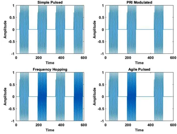
I S S N : 2 6 3 6 - 6 0 7 X 3 | P a g e waveforms (Sharma et al., 2014) and design of cost-efficient frequency hopping radar waveform for range and Doppler estimation (Nuss et al., 2016). Agile pulsed radar signal is a hybrid signal of PRI modulated signal and frequency hopping signal. The time-plot of these radar signals discussed is presented in Figure 1 based on a designed radar signals generation algorithm in this paper.

Figure 1. The time plots for airborne radar signals

Firstly, the plot presented in Figure 1 is for illustration and comparison purposes as PRI in the real world is much higher in order to obtain a longer unambiguous range (Skolnik, 2008). Each of the blue lines shown in Figure 1 depicts a sinusoidal modulation during the PW with its frequency depending on the desired signal. It is seen that for the simple pulsed radar signal of Figure 1; the sinusoid is similar (due to same colour shade) and the time between them is constant depicting a constant time and frequency parameters. As for the PRI modulated, the sinusoid is similar but the time between them is different indicating a constant frequency but changing PRI parameter. The sinusoid is different for the frequency hopping signal but time between them is constant and therefore indicating the opposite of the PRI modulated signal. The agile pulsed signal has different sinusoid and different time in between them indicating the changing time and frequency parameter. The traditional Fast Fourier Transform (FFT) can give the frequency parameters but not when they occur and how many times they occur for the duration of the observation. This is what led to the development of the time-frequency distribution (TFD) capable of obtaining the joint time-time-frequency representation (Boashash, 2016).

3. Methodology

Time-frequency distribution is a way of representing the energy distribution of a signal over the time-frequency domain. The short time Fourier transform (STFT) was used as the TFD in this paper due to its low computational complexity. It is the oldest TFD of the classical Fourier transform origin that uses sliding window to localise the content of the signal in the joint time frequency domain (Gabor, 1946). It is mathematically given in (1).

𝐹𝑧𝑤(t, f) = Ft→f{z(τ)w(τ − t)} (1)

where, 𝐹𝑧𝑤 is the STFT, Ft→f { . . } denotes taking Fourier transform of the expression in the bracket, w(τ) is the

sliding window time, z(τ) is the analytic version of the signal (s(τ)) and τ is the arbitral time parameter for the Fourier transformation. Time-frequency signal analysis requires the use of the analytic signal which will have

(4)

4 | P a g e I S S N : 2 6 3 6 - 6 0 7 X

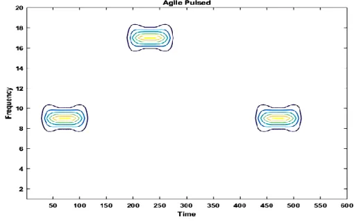
neither any aliasing effect nor frequency artefacts and can easily be obtained using Hilbert transform (Boashash, 1998). The square magnitude of the STFT was used for the analysis in order to reduce the effect of noise. A graphical interpretation of this STFT is given in Figure 2 for the agile pulsed radar signal presented in Figure 1. The agile pulsed is selected due to its varying time and frequency characteristics and hence would represent the other remaining signals.

Figure 2. Joint time-frequency plot of an agile pulsed radar signal

It is clearly seen from the contour plot of Figure 2 that changing time and frequency parameter for an agile pulsed radar signal was correctly captured by the STFT. The power from the STFT was obtained in Figure 2 from the internal line where higher power was recorded for lines closed to the centre. The other three remaining test signals were captured accurately by this STFT. In order to estimate time and frequency parameter respectively, the IP and IF were obtained from the TFR (such as that of Figure 2) through (2) and (3) respectively.

𝑃𝑖(𝑡) = max(𝐹𝑧𝑤(t, f)) , (2)

𝑓𝑖(𝑡) = max_𝑓 (𝐹𝑧𝑤(t, f)), (3)

where, 𝐹𝑧𝑤is the obtained STFT representation.

The IP and IF reduces the TFR of three dimensions of power, frequency and time to two dimensions of power and time for IP and frequency and time for IF for easier signal processing. The IP depicts the maximum power based on the search along the frequency axis while IF corresponds to the frequency location of this maximum power along this search. Hence the only difference between the equations (2) and (3) is ‘f’ below the max to indicate frequency location.

The time parameters; PW, 1st_{and 2}nd_{PRI (PRI}₁_{and PRI}₂_{) are gotten from IP estimation using a basic} algorithm formed from common loop statements based on a chosen threshold. Twelve and half percentile threshold was used in this work in order to cater for the unconventional signals of frequency hopping and agile pulsed. The frequency parameters; first and second carrier frequency (F1 and F2) were gotten from the IF simply by finding the average sample points on the frequency axis during the corresponding obtained PW time from the IP estimation.

4. Results and Discussion

For analysis of the received signals, it was assumed that the signal was de-interleaved and down converted to achieve a current standard sampling frequency of 100 MHz based on Agilent P-Series Power meters for radar signal surveillance (Agilent Technologies, 2014). For the frequency hopping signals, hopping of two frequencies was considered with each pulse containing different frequency while for the PRI modulated signal; PRI of two intervals and two positions were considered. The agile pulse considered was like a combination of the two signals as already stated. For performance analysis, the noise environment was modelled AWGN. This noise is very common and suitable for microwave communications environment like radar telecommunications where worst case scenario is assumed (Ziemer & Peterson, 2001).

(5)

I S S N : 2 6 3 6 - 6 0 7 X 5 | P a g e The classification performance was done through a Monte Carlo simulation setup whereby two loops involving signal-to-noise ratio (SNR) and iteration controls were used. A standard iteration of 100 loops for each SNR was used in this work while the formula used for the SNR (in decibel) is given in (4).

𝑆𝑁𝑅(𝑑𝐵) = 10 log𝑃𝑠

𝑃𝑛, (4)

where: 𝑃𝑠 is the signal power and 𝑃𝑛 is the noise power.

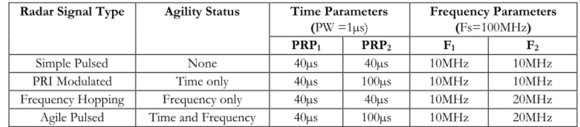
The table of parameters for the test radar signals used in this work is shown in Table 1. Table 1. Test airborne radar signals

Radar Signal Type Agility Status Time Parameters (PW =1µs)

Frequency Parameters (Fs=100MHz)

PRP1 PRP2 F1 F2

Simple Pulsed None 40µs 40µs 10MHz 10MHz

PRI Modulated Time only 40µs 100µs 10MHz 10MHz

Frequency Hopping Frequency only 40µs 40µs 10MHz 20MHz Agile Pulsed Time and Frequency 40µs 100µs 10MHz 20MHz

PW of 1µs from Table 1 was used due to lack of sophisticated intra pulse modulation (like linear frequency and phase shift keying modulations) (Wiley, 2006) while PRI of 40µs and 100µs corresponds to small and medium range of 6Km and 15Km respectively (Stimson, 1998). Carrier frequencies presented in Table 1 were selected within the Nyquist sampling theory (i.e. carrier frequencies must be less than or equal to half the sampling frequency to avoid aliasing) (Shenoi, 2006).

A rule-based classifier was designed based on the changing four parameter inputs (PRI1, PRI2, F1 and F2) in order to obtain correct classification accuracy with a 10% error allowance which gives an output based on five possible outcomes. Summary of this classifier is given in the Table 2.

Table 2. Classifier design

Parameter Limits Code No Radar Signal

Time Limit Frequency Limit

PRI1min≤ PRI2 ≤ PRI1max F1max ≤ F2 ≤ F1max 1 Simple Pulsed

PRI1max < PRI2 F1max ≤ F2 ≤ F1max 2 PRI Modulated

PRI1max ≤ PRI2 ≤ PRI1max F1max < F2 3 Frequency Hopping

PRI1max < PRI2 F1max< F2 4 Agile Pulsed

Else Else 5 Unknown Signal

where,

PRI1min= PRI1 – 0.1 ∗ PRI1 (5)

PRI1max= PRI1+ 0.1 ∗ PRI1 (6)

F1min= F1 – 0.1 ∗ F1 (7)

F1max= F1+ 0.1 ∗ F1 (8)

Equations (5) - (8) gives the mathematical definitions for the limits presented in Table 2 in line with the earlier mentioned 10% (0.1) error allowance. A radar signal must meet both the time and frequency parameter limits as defined in Table 2 to meet the classification requirements. The code no is the equivalent number representation of the radar signal in MATLAB due to the fact that MATLAB doesn’t recognize alphabet classifications based on this classifier construct. Hence, POCI of each signal was obtained after generation of test signals and addition of AWGN for SNR range of -18dB to 17dB.

The POCI is given by the formula in (9).

𝑃𝑂𝐶𝐼 (%) = 𝑁𝐶𝐶

𝑁𝑇𝐶 ∗ 100% (9)

where, 𝑁𝐶𝐶 is number of correct classifications and 𝑁𝑇𝐶 is the number of total classifications (equivalent to the

standard number of 100 iterations).

(6)

6 | P a g e I S S N : 2 6 3 6 - 6 0 7 X

Table 3. Monte Carlo Simulation Results for POCI

SNR (dB) Simple Pulsed PRI Modulated Frequency Hopping Agile Pulsed

-18 5 2 60 35 -17 1 10 51 56 -16 0 40 16 89 -15 3 44 25 93 -14 30 60 77 99 -13 43 46 94 99 -12 50 66 95 100 -11 48 69 100 100 -10 68 75 100 100 -9 64 69 100 100 -8 66 84 100 100 -7 68 83 100 100 -6 86 87 100 100 -5 89 96 100 100 -4 86 98 100 100 -3 94 99 100 100 -2 93 99 100 100 -1 98 100 100 100 0 99 100 100 100 1 99 100 100 100 2 100 100 100 100 3 100 100 100 100 4 100 100 100 100 5 100 100 100 100 6 100 100 100 100 7 100 100 100 100 8 100 100 100 100 9 100 100 100 100 10 100 100 100 100 11 100 100 100 100 12 100 100 100 100 13 100 100 100 100 14 100 100 100 100 15 100 100 100 100 16 100 100 100 100 17 100 100 100 100

The minimum SNR required for classification accuracy of 99% from Table 3 is 0dB, -2dB, -11dB, -13dB for simple pulsed, PRI modulated, frequency hopping and agile pulsed radar signals respectively. The difference in POCI can be attributed to the different time and frequency characteristics in each signal and limits set by the classifier in order to achieve correct classifications. Signals with upper and lower limits took higher SNR to achieve POCI of 99% even more so when these limits were present in both time and frequency parameters. As

(7)

I S S N : 2 6 3 6 - 6 0 7 X 7 | P a g e such agile pulsed radar signal achieved perfect identification accuracy at minimum SNR of -12dB while a difference of 14dB was observed for the worst case scenario for the simple pulsed radar signal to achieving similar feat. A graphical representation of Table 3 is shown in Figure 3 for further discussion and better result presentation.

Figure 3. Monte Carlo Simulation Results for POCI of Radar Signals

Two main points were further observed and deduced from Figure 3. Firstly, the slight zigzag nature of classification results before constant POCI; which is attributed to random characteristics of AWGN model. Secondly, the minimum SNR of 0dB for classification results is further ascertained for which POCI of 99% was obtained irrespective on the input signal within the scope of this work.

5. Conclusion

This paper described an agile analysis algorithm based on STFT for accurate classification of any intercepted airborne radar signal based on varying pulse characteristics. The signal may be of constant time and frequency parameters (simple pulsed), varying time parameter only (PRI modulated), varying frequency parameter only (frequency hopping) or varying time and frequency parameters (agile pulsed). Monte Carlo simulation set up for signal identification was carried out in the presence of AWGN within SNR range of -18dB to 17dB in order to determine the performance of the methodology designed and adopted in this paper. As a result of this simulation setup, a relationship was achieved between POCI and the SNR range.

It was established that the presence of upper or lower limits or both in the classification rules affected the POCI result. As such, identification of agile pulsed signal performed best with the presence of just lower limits in both time and frequency, followed by frequency hopping signal due to presence of both limits in its time with having just lower limit in frequency. The next was PRI modulated with the presence of lower limit in time but both limits in frequency with simple pulsed performing poorest due to having both limits in time and frequency. However, irrespective of intercepted radar signal, the results obtained in this paper indicated its correct identification at a good SNR range of equal to or greater than 0dB based on the designed algorithm.

It is therefore seen that the designed algorithm used in this paper may be deployed in the field of EW for aerial battle and electronic reconnaissance where intercepted/captured radar signal may be analysed to determine its pulse changing characteristics. These analyses will also provide further insight into the intention of the intercepted radar emitter where radar signals of constant time and frequency parameters are generally non-hostile while further investigation would have to be carried out for those of non-constant time and frequency parameters. The developed algorithm can also form an essential part of an electronic counter system capable of reducing the effectiveness of weapon guidance devices through counter effective measures such as jamming based on the correct signal identification.

(8)

8 | P a g e I S S N : 2 6 3 6 - 6 0 7 X

Conflict of Interests

The authors declare that there is no conflict of interests regarding the publication of this paper. References

Adamy, D. L. (2001). EW 101: A First Course in Electronic Warfare. Boston: Artech House.

Agilent Technologies, Inc. (2014). Agilent Radar Measurements: Application Note. USA: Agilent Technologies, p18.

Ahmad, A. A., & Sha’ameri, A. Z. (2015). Classification of Airborne Radar Signals based on Pulse Feature Estimation using Time-Frequency Analysis. Science & Technology Research Institute for Defence, p103.

Ahmad, A. A., Ayeni, J. B., & Kamal, S. M. (2015). Determination of the pulse repetition interval (PRI) agility of an incoming radar emitter signal using instantaneous power analysis. AFRICON, 2015, 1-4.

Boashash, B. (1988). Note on the use of the Wigner distribution for time-frequency signal analysis. IEEE Transactions on Acoustics, Speech, and Signal Processing, 36(9), 1518-1521.

Boashash, B. (2016). Time-frequency signal analysis and processing: a comprehensive reference, 2nd Ed. Oxford: Academic Press.

Cao, R., Cao, J., Mei, J. P., Yin, C., & Huang, X. (2018). Radar emitter identification with bispectrum and hierarchical extreme learning machine. Multimedia Tools and Applications, 1-18.

Daniyan, A., Ahmad, A. A., & Gabriel, D. O. (2015). Selection of window for inter-pulse analysis of simple pulsed radar signal using the short time Fourier transform. International Journal of Engineering & Technology, 4(4), 531.

Elsworth, A. T. (2010). Electronic warfare. New York: Nova Science Publishers.

Erdogan, A. Y., Gulum, T. O., Durak-Ata, L., Yildirim, T., & Pace, P. E. (2017). FMCW Signal Detection and Parameter Extraction by Cross Wigner–Hough Transform. IEEE Transactions on Aerospace and Electronic Systems, 53(1), 334-344.

Gabor, D. (1946). Theory of Communication. Journal of the Institution of Electrical Engineering part III, 93(26): 429-457.

Li, L., & Jiang, L., (2014). Recognition of polyphase coded signals using time-frequency rate distribution. In 2014 IEEE Workshop on Statistical Signal Processing (SSP), 484-487.

Neri, F. (2006). Introduction to electronic defense systems. North Carolina: SciTech Publishing.

Nuss, B., Fink, J., & Jondral, F. (2016). Cost efficient frequency hopping radar waveform for range and Doppler estimation. In 2016 17th IEEE International Radar Symposium (IRS), 1-4.

Pace, P. E. (2009). Detecting and classifying low probability of intercept radar. Boston: Artech House.

Sedivy, P. (2013). Radar PRF staggering and agility control maximizing overall blind speed. Conference onMicrowave Techniques (COMITE), 197-200.

Sharma, G. V. K., Srihari, P., & Rajeswari, K. R. (2014). MIMO radar ambiguity analysis of frequency hopping pulse waveforms. In 2014 IEEE Radar Conference, 1241-1246.

Shenoi, B. A. (2006). Introduction to Digital Signal Processing and Filter Design. New Jersey: John Wiley & Sons Inc. Skolnik, M. I. (2008). Radar handbook, 3rd_{Edition. New York: McGraw Hill Companies.}

Stevens, L., & Schuckers, S. A. (2016). Low Probability of Intercept Frequency Hopping Signal Characterization Comparison using the Spectrogram and the Scalogram. Global Journal of Research in Engineering, 16(2).

Stimson, G. W. (1998). Introduction to airborne radar. SciTech Pub

Tekanyi, A. M. S., Abubilal, K. A., Saliu, A. S., Yahaya, S. O., & Abubakar, H. A. (2017). Algorithm for the Estimation of Time and Frequency Parameters of a Simple Pulsed Radar Signal. ATBU Journal of Science, Technology and Education, 5(4), 30-41. Wiley, R. G. (2006). ELINT: The interception and analysis of radar signals. Boston: Artech House

Wolff, C. (2009). Radar Tutorial (Book 1): Radar Basics. Western Pommerania: Achatweg3

Zhang, J., Li, Y., & Yin, J. (2017). Modulation classification method for frequency modulation signals based on the time–frequency distribution and CNN. IET Radar, Sonar & Navigation. 12 (2), 244-249.

Ziemer, R. E., & Peterson, R. L. (2001). Introduction to Digital Communication. Prentice-Hall International, Upper Saddle River, New Jersey.