GATE Monte Carlo Simulations in a Cloud Computing Environment

(1)

UNLV Theses/Dissertations/Professional Papers/Capstones

8-1-2014

GATE Monte Carlo Simulations in a Cloud

Computing Environment

Blake Austin Rowedder

University of Nevada, Las Vegas, [email protected]

Follow this and additional works at:http://digitalscholarship.unlv.edu/thesesdissertations

Part of theComputer Sciences Commons,Digital Communications and Networking Commons, Medical Sciences Commons,Oncology Commons, and thePhysics Commons

This Thesis is brought to you for free and open access by Digital Scholarship@UNLV. It has been accepted for inclusion in UNLV Theses/ Dissertations/Professional Papers/Capstones by an authorized administrator of Digital Scholarship@UNLV. For more information, please contact [email protected].

Repository Citation

Rowedder, Blake Austin, "GATE Monte Carlo Simulations in a Cloud Computing Environment" (2014).UNLV Theses/Dissertations/ Professional Papers/Capstones.Paper 2212.

(2)

i

GATE MONTE CARLO SIMULATION IN A CLOUD

COMPUTING ENVIRONMENT

By

Blake Austin Rowedder

Bachelor of Science in Physics University of Minnesota – Twin Cities

2012

A thesis submitted in partial fulfillment of the requirements for the

Master of Science - Health Physics

Department of Health Physics and Diagnostic Sciences School of Allied Health Sciences

Division of Health Sciences The Graduate College

University of Nevada, Las Vegas August 2014

(3)

ii

(4)

ii

THE GRADUATE COLLEGE

We recommend the thesis prepared under our supervision by

Blake Austin Rowedder

entitled

Gate Monte Carlo Simulation in a Cloud Computing Environment

is approved in partial fulfillment of the requirements for the degree of

Master of Science - Health Physics

Department of Health Physics and Diagnostic Sciences

Yu Kuang, Ph.D., Committee Chair Bing Ma, Ph.D., Committee Member Gary Cerefice, Ph.D., Committee Member

Janet Dufek, Ph.D., Graduate College Representative

Kathryn Hausbeck Korgan, Ph.D., Interim Dean of the Graduate College

(5)

iii

ABSTRACT

The GEANT4-based GATE is a unique and powerful Monte Carlo (MC) platform, which provides a single code library allowing the simulation of specific medical physics applications, e.g. PET, SPECT, CT, radiotherapy, and hadron therapy. However, this rigorous yet flexible platform is used only sparingly in the clinic due to its lengthy calculation time. By accessing the powerful computational resources of a cloud computing environment, GATE’s runtime can be significantly reduced to clinically feasible levels without the sizable investment of a local high performance cluster. This study investigated a reliable and efficient execution of GATE MC simulations using a commercial cloud computing services. Amazon’s Elastic Compute Cloud was used to launch several nodes equipped with GATE. Job data was initially broken up on the local computer, then uploaded to the worker nodes on the cloud. The results were automatically downloaded and aggregated on the local computer for display and analysis. Five simulations were repeated for every cluster size between 1 and 20 nodes. Ultimately, increasing cluster size resulted in a decrease in calculation time that could be expressed with an inverse power model. Comparing the benchmark results to the published values and error margins indicated that the simulation results were not affected by the cluster size and thus that integrity of a calculation is preserved in a cloud computing environment. The runtime of a 53 minute long simulation was decreased to 3.11 minutes when run on a 20-node cluster. The ability to improve the speed of simulation suggests that fast MC simulations are viable

(6)

iv

for imaging and radiotherapy applications. With high power computing continuing to lower in price and accessibility, implementing Monte Carlo techniques with cloud computing for clinical applications will continue to become more attractive.

(7)

v

ACKNOWLEDGEMENTS

This work could not have been completed without the help and insight of several individuals. First of all, I would like to thank my advisor Dr. Kuang for his support and expertise. His direction and encouragement over the past two years allowed my thesis to move from an idea to a completed study. I would also like to thank Drs. Cerefice, Dufek, and Ma, my thesis examination committee members, for graciously sharing their time and help. I would also like to thank Drs. Hui Wang and Xia Li, whose guidance and patience played an integral part in me being able to complete this work.

(8)

vi

LIST OF TABLES

Table 1. PET output compared to expected benchmarked data ... 26

Table 2. Runtime for each cluster size of PET benchmark ... 27

Table 3. SPECT output compared to expected benchmark data ... 29

Table 4. Runtime for each cluster size of SPECT benchmark ... 30

Table 5: Runtime for each cluster size of gamma simulation ... 32

Table 6. Runtime for each cluster size of radiotherapy simulation ... 37

Table 7. Runtime for each cluster size of proton beam simulation ... 40

Table 8. PET Benchmark repeated on 1 node ... 44

Table 9. Time taken to run simulations under identical conditions ... 44

(11)

ix

LIST OF FIGURES

Figure 1. Workflow diagram of basic distributed computing ... 7

Figure 2. Workflow diagram ... 14

Figure 3. Generated image of PET scan simulation ... 17

Figure 4. SPECT simulation image ... 19

Figure 5. Sample image from the POPI patient CT ... 22

Figure 6. Graphical output of PET simulation on 15-node cluster ... 24

Figure 7. Decay curves for various cluster sizes ... 25

Figure 8. Graph of the relationship of cluster size and time of PET simulation ... 28

Figure 9. Graph of relationship between cluster size and time of SPECT simulation ... 30

Figure 10. Dose distribution output of the gamma beam ... 32

Figure 11. Graph of the relationship of cluster size and time of gamma simulation ... 33

Figure 12. Output for radiotherapy simulation on 1 node ... 35

Figure 13. Output for radiotherapy simulation on 2 nodes ... 36

Figure 16. Graph of the relationship of cluster size and time of radiotherapy simulation ... 38

Figure 17. Dose distribution on 2 node cluster ... 39

Figure 20. Graph of the relationship of cluster size and time of simulation ... 41

Figure 21. Total cluster runtime for PET benchmark ... 43

(12)

1

CHAPTER 1 INTRODUCTION

While Monte Carlo methods have existed roughly since the origin of computers, their computationally intensive characteristics have hindered their more widespread use in clinical radiotherapy dose calculations.1 Studies have shown Monte Carlo techniques can provide more accurate dose distribution predictions than other methods.2,3 However, Monte Carlo is used only sparingly in clinics, despite the fact that it offers a rigorous yet flexible tool for modeling the stochastic nature of radiation propagating through matter. The biggest barrier for wider use is that a Monte Carlo dose calculation carried out on a single processor has a clinically unacceptable runtime, ranging from hours to even days. This has rendered Monte Carlo methods largely infeasible for clinical dosimetry calculations in the past.

However, the rise of new cloud computing technologies has made high computational power available without investing in a personal computing cluster. This emerging technology alters the economics and feasibility of introducing Monte Carlo techniques in clinics because it alleviates the expense of computer purchase, storage, maintenance, and upgrades for a cluster.4 This research serves as a proof-of-concept of the performance of a distributed processing framework for radiation physics calculations in a cloud computing environment.

(13)

2

The potential of Monte Carlo calculations has captured the field of medical physics’ attention and is the subject of a great deal of research. Several studies have demonstrated its superior capabilities for dose calculations.5,6 Some have specifically focused on the GATE software.7,8 Others have explored the use of cloud computing for making dosimetric calculations for various Monte Carlo packages, and have also studied the cost structure of doing so.9,10,11

The GEANT4-based GATE is a unique and powerful Monte Carlo platform, which provides a single code library allowing the simulation of several specific medical physics applications, such as PET, SPECT, CT, internal and external radiotherapy, and hadron therapy.3,12,13 However, its lengthy runtime hinders its routine use in the clinic. Reducing its computing time is therefore of great importance. Thus, a commercial cloud compute service is well suited for GATE simulation, both in terms of cost and efficiency. Yet to date none have attempted to run GATE specifically in a commercial cloud computing environment.

This study acts as a proof-of-concept that GATE Monte Carlo simulations are viable in a commercial cloud computing environment. Five simulations representing different medical physics applications were run for a variety of cluster sizes and the achieved simulation speed-up and associated costs were recorded. The simulations were repeated for all cluster sizes ranging between one and twenty nodes. Across all five simulations, output was found to be independent of cluster size. For the first simulation, redundant calculations were performed to verify repeatability. While there was variation in runtime, this yielded virtually identical results, which further suggests the consistency and repeatability of running Monte Carlo in this manner. Any incidents of node failure or

(14)

3

abnormal results were recorded to examine reliability, which occurred a total of five times. Given that around 1050 nodes were initialized and used over the course of this study, this is a failure rate of roughly 0.48%. The decrease in runtime observed from increasing cluster size up to 20 nodes was established to be an inverse power relationship.

(15)

4

CHAPTER 2 BACKGROUND

2.1 Monte Carlo Method

2.1.1 Basics of Monte Carlo Method

Monte Carlo techniques differ from other computation algorithms in their use of random number sampling. Large sample sizes allow the stochastic nature of the random sampling to model the statistical fluctuations of reality. It is generally most useful in scenarios when it is impossible to obtain a closed-form expression or deterministic algorithm. This makes it well-suited for modeling the propagation of particles through matter and the dose it distributes, given its random nature. Imagine, for example, a photon traveling through tissue. It has a unique cross-section of its probability to interact by photoelectric or Compton scattering for each unit distance it travels through the tissue. Random sampling can dictate what, how, and where it interacts. The initial photon in this case is called a primary particle, and all of the electrons or photons it frees or creates from interactions are referred to as secondary particles. A Monte Carlo dose calculation will simulate the unique tracks of a large number of individual particles for a given medium geometry to simulate the deposition of energy within the medium. There are many parameters and assumptions that can be made in a Monte Carlo calculation based on the

(16)

5

desired time of the simulation and the level of accuracy needed. Simply increasing the number of primary particles will increase the accuracy of the results by mitigating the statistical fluctuations of random numbers, but the time of simulation will increase accordingly. Another method used to decrease computation demand is setting a cut-off energy. The calculation will stop following a particle after its energy falls below a certain energy, thus sparing it from carrying out several more low-energy interactions that will have negligible effects on dose.14

2.1.2 Geant4 and GATE

Geant4 (for GEometry ANd Tracking) is a Monte Carlo platform designed to model particles passing through and interacting with matter.15 While useful across many fields of physics, it was integrated into a Monte Carlo simulation toolkit designed by the OpenGate collaboration to create GATE (the Geant4 Application for Tomographic Emission) specifically for medical physics applications. As its acronym suggests, its initial release in 2004 was designed for modeling PET and SPECT. It has since expanded into GATE V6, with expanded flexibility allowing for modeling of nearly all relevant scenarios imaginable in the realm of medical physics.15_{Ultimately, GATE is a tailored user interface to support} the use of GEANT4 physics code for medical physics applications.

There are several other Monte Carlo platforms for dosimetry, such as MCNPX, FLUKA, TOPAS, and XVMC.16 GATE is unique in being the only platform allowing for radiotherapy, dosimetry, and imaging application in the same environment.16 This, along with its open-source status, make GATE an ideal platform for use both in a clinical setting and a research setting. Radiotherapy treatment planning requires calculating the

(17)

6

distribution of absorbed dose inside a patient. GATE is versatile enough to do this, regardless if it is a photon, electron, proton, or carbon beam or if it is delivered via pencil beam, broad beam, beam scanning, or brachytherapy. It can also handle the needs of diagnostic imaging applications, where Monte Carlo calculations can be useful for system design, evaluating detection probabilities, or measuring the absorbed dose to assess risk-benefit of a procedure like a CT, PET, or SPECT. The advent of on-board imaging and other techniques that intertwine imaging and therapy suggests the need for a Monte Carlo platform that can model both applications, and GATE fits this need well.

2.2 Distributed Computing

2.2.1 Basics of Distributed Computing

A solution to Monte Carlo’s lengthy runtime has been found in distributed computing. Distributed computing is a program model for processing large data sets in relatively small amounts of time. This is accomplished by using a large number of individual computers, referred to as nodes. These nodes are collectively referred to as a cluster if they are all on the same local network and use similar hardware. The intent of distributed computing is to divide the work into many small fragments, each of which is executed on any node in the cluster. A master node controls the process of dividing the work and aggregating the results. Distributed computing is not usable for every computational problem, but is most useful for situations where a large volume of computations needs to be completed, but the computations can be divided into parts that

(18)

7

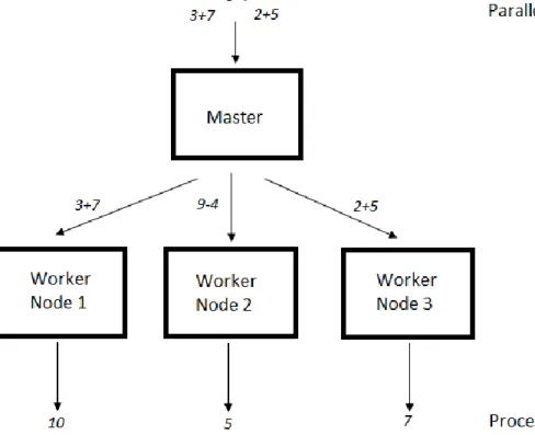
are all independently solvable. A diagram of this concept is shown in Figure 1, where a “parallelizable problem” consisting of a few math problems is divided into three parts on the master node and solved simultaneously on three worker nodes. The solutions are stored on their respective worker node until the entire problem is complete, and then sent back to the master node to be compiled. Monte Carlo simulations are well suited for distributed computing because the particle histories are completely independent of one another, thus no communication is needed between processes.9_{This means it is highly parallelizable} and calculations do not need to maintain data or timing synchronization during execution so it can easily be divided to many nodes. The solutions to these many particle histories are then compiled to estimate a dose depth distribution of the incident radiation.

(19)

8

While distributed computing is well suited for Monte Carlo methods, it needs large computing resources in order to have clinically acceptable run times. This requires an investment in a sizeable infrastructure of computers as well as the associated utility, upgrade, maintenance, and personnel costs. Keyes4 estimated the cost of a personal cluster to be $1000 per node plus roughly $200 per year per node for maintenance costs. Thus, the limiting factor for clinics in producing highly accurate Monte Carlo radiation dose calculations in reasonable time scales is mainly cost. Even ignoring personnel, utility, insurance, and housings costs of a personal cluster, Keyes estimated using AWS would cost 80% less over a 3 year time span.4

2.2.2 Cloud Computing

Cloud computing is ultimately the same concept as distributed computing, except instead of using a cluster of computers in close physical proximity to the user, a cluster of computers is accessed remotely via the internet. In academia or industry this method is frequently used as a method to access private off-site clusters, but in this study the focus is on commercial cloud computing. Providers of commercial cloud computing resources typically own warehouses full of publicly available nodes that can be accessed remotely with nothing more than a credit card and internet access. These providers offer online computing resources scalable to user’s needs using a pay-as-you-go hourly fashion that is competitively priced due to the economy of scale of their product. Since the computational resources can be scaled to meet daily fluctuations in demand, the user only pays for the computers they use while they use them, opposed to a local cluster that may be overclocked

(20)

9

during business hours and unused overnight. Additionally, the details of the network and hardware architecture are transparent to the user, making it easily accessible.

2.3 Significance of Cloud Computing with Monte Carlo

Even the most comprehensive deterministic dose calculation algorithms produce errors under certain situations, such as air-tissue inhomogeneity.7 A testament of the reliability of Monte Carlo is found in the fact that it is often used as the benchmark when comparing and testing these algorithms. Unfortunately it used infrequently in actual clinics because of its high computational demand. A clinic cannot allow for one of their treatment planning machines to be tied up for hours on a single calculation. Alternatively, they don’t have the space and finances to justify implementing their own local cluster of computers.4 Cloud computing offers an alternative way for clinics to run Monte Carlo simulations without tying up their own computers all day, or making the sizable investment in a personal cluster. As high speed computing becomes cheaper and more readily available, it becomes more and more attractive to use Monte Carlo itself to carry out routine dose measurements in a clinical setting.

It is worth discussing the implications of this research beyond a clinical setting. As any researcher is well aware, funding and resources cause most limitations in what research can be carried out. Even as free software, running simulations with GATE is limited to

(21)

10

those with access to high-power computers. Amazon’s EC2 offers unprecedented ease of access to powerful computing resources. The only requirement for use are internet access and a credit card. This opens the door for researchers to do a variety of simulations research without needing access to a local cluster.

(22)

11

CHAPTER 3 METHODS AND MATERIALS

3.1 GATE V6.1 and Jobsplitter

For this study, the local computer used a Ubuntu operating system version 10.04.3 LTS and the cloud computers used Ubuntu 10.10 version.17_{Each was installed with GATE} V6, which is the newest version of the GATE software and is available free from the OpenGATE Collaboration website.3 This version contains the commands Job Splitter and File Merger that make it usable in a cluster environment. A simulation in GATE is contained in one or more job files known as macros. These describe the geometry of the phantom, detectors, source or anything else in the ‘world’, as well as declaring which physics processes to simulate and what information to store or visualize. Usually a simulation is described in a main macro that references several other smaller macros describing materials, phantom geometry, etc. The Job Splitter function takes a given main macro and all the smaller macros it references, combines it into one macro file, and divides the work into any number of macros to send to individual nodes. Each macro file it creates is self-contained, so only one file needs to be sent to each node without all of the peripheral files that the original main macro references. This allows for breaking up a single job into several smaller, self-contained job files to send to the individual nodes. The File Merger command essentially performs the opposite function of Job Splitter; it takes the individual outputs of all the smaller macro jobs and compiles it into a single results file. These

(23)

12

commands were used to prepare jobs to be completed in the cloud, and to aggregate the results.

3.2 Amazon Web Services and Elastic Compute Cloud

One of the various web-based resources offered by Amazon Web Services (AWS) is Elastic Compute Cloud (EC2).18 EC2 allows users to create and connect to a computer of their specification on command, which is referred to as an instance. EC2 has a variety of different nodes available based on the needs of users. The hourly rates for each node varies based on the combination of processor, memory, and RAM desired. The C1.medium instance is a moderately powerful computer that is optimized for highly computational work without sacrificing affordability. For the sake of consistency, this is the only instance type that was used to collect data for this experiment. It uses an Intel Xeon E5506 processor with 2.13 GHz clock speed, has 1.7 MB of memory, and costs $0.145 per hour. Amazon rates its processors in terms of EC2 Compute Units, which they state is roughly equivalent to a 1.0-1.2 2007 Opteron processor.18 Each virtual machine has an operating system loaded onto it with user configured software using an Amazon Machine Image (AMI). AMI’s are chosen from Amazon’s pre-configured set. Once an instance is running, it has a unique IP and domain and is effectively its own unique computer, hence the name virtual machine.

(24)

13

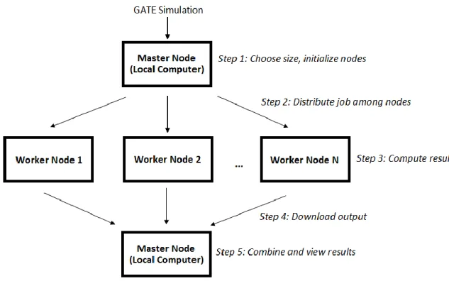
A virtual cluster is built by requesting multiple virtual nodes. The size of the cluster can be scaled on demand based on the magnitude of calculations needed. The cluster workflow in this study is unique in that the local computer also acts as the master node. The local computer performs the Job Splitter and File Merger tasks, but no actual calculations are carried out on it. The user requests N nodes to carry out the calculation, and the worker nodes are initialized on the cloud. Then the calculation parameters are established and the work is distributed into N self-contained job files on the local computer. For example, on a 5 node cluster a 100 particle calculation would be broken into 20 particle runs. Each of these files is uploaded to its respective node and the command to begin the Monte Carlo calculation is sent to each simultaneously. After the dose calculations are complete, the dose files are downloaded to the local computer and combined into a single output file, which is then ready to be viewed. A program to automate the process of dividing up the GATE job and distributing it to N nodes was developed in Python using the BOTO library. BOTO is a python library specifically designed to interface with Amazon Web Services.19

Each of these individual simulations was run several times under varying conditions. The number of nodes in the cluster was varied from 1 to 20 for repeated trials of the same simulation in order to establish the relationship between number of nodes and time of simulation. Additionally, the output was compared to verify that the integrity of the results is not affected by the number of nodes. The relationship between cluster size and price for a simulation was also investigated.

Python commands from the BOTO library are used to initialize each node. Then the job file is split into self-contained partial jobs that are transferred to the worker nodes

(25)

14

with an SSH connection. Each node would automatically boot GATE, load the environmental variables, and run the job upon receiving commands from the master node. After finishing the calculations, the worker node would push their files to the local computer and aggregate the partial files into a single file. Code was developed to automate the entirety of this process for the ease of the end user. This required an AMI with GATE fully installed and boot script opening and configuring it upon initialization. It additionally requires a Python program run on the local computer to automate the process of initializing the cluster, connecting to the master node, sending the job data, and getting the results. Automation allows for faster data collection and for arbitrarily large cluster sizes without

increasing workload on the user. Figure 2 depicts a diagram of the workflow of this entire process.

(26)

15

Amazon’s EC2 has a 20 node limit for simultaneously running on-demand instances from a single user. Preliminary data suggested that a cluster size upper limit of 20 would be sufficient to establish its relationship with run time. Thus, the effects of cluster sizes larger than 20 nodes were not explored.

Two repeats were carried out for 1, 3, 5, 15, and 20 node cluster sizes for the first simulation, the PET Benchmark, to assure that the results are repeatable. Given that this is primarily a proof-of-concept study, a more rigorous examination of repeatability was not carried out. In subsequent simulations, only 1 repeat cluster size was carried out unless the results appear erroneous. This was carried out for each simulation to confirm there were no simulation-specific problems with repeatability. As for reliability, it is worth noting that Amazon’s virtual instances do at times fail. This is unavoidable from the user end so wariness was used when collecting data. Any uncharacteristic results warranted investigation and repeat runs.

3.4 The Simulations

In order to obtain a robust assessment of GATE’s performance in a cloud computing environment, five different simulations were run. Each simulation was repeated for every cluster size from 1 to 20. There were two facets to the data collected from each run. The runtime required for the cluster to finish was recorded, and the resulting output of the simulation was saved. For the purpose of this study, runtime only includes the actual time taken by the GATE simulation. It is important to note that it does not include the time

(27)

16

taken to upload the initial job information to the cloud or to download the results onto the local machine. Since trials were not always carried out under the same conditions of internet speed and connection, this was deemed to add too high of a variable and fluctuation to the total runtime. Since the time taken to upload and download information to the cloud is an important part to consider when assessing the feasibility of cloud computing, the estimated time increase and its ramifications are still explored in the discussion. GATE is packaged with a PET and SPECT Benchmark. Upon configuring GATE with a system, it is recommended to run these benchmark simulations and compare the output to the known results to verify that it is installed correctly. Given that these simulations were designed as benchmarks and have readily available output data for comparison, they are excellent choices for inclusion in this research.20 Their inclusion allowed for a statistical comparison of their numerical results on various cluster sizes to the well documented benchmark results expected. The other three simulations chosen were a basic gamma beam, a linac photon beam, and a proton beam incident on a CT image. These simulations had mostly visual and graphical outputs and no well-known benchmark data to compare it to. Thus, no formal statistical analysis was carried out to ensure consistent results. Overall, these five simulations cover a broad spectrum of clinical scenarios to illustrate the versatility of GATE.

3.4.1 PET Benchmark

The PET benchmark simulation is packaged with the GATE software to be run after installation in order to verify that it is installed correctly. This means that standard data is available for comparison to test the integrity of running GATE in a cloud computing

(28)

17

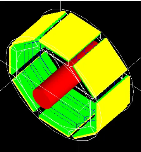
environment. This simulation models a whole-body scanner that is described in a macro file named camera.mac. It does not model any existing system, but instead models an ideal scanner with eight detector heads.20 Figure 3 shows an image generated by this simulation in GATE to demonstrate the geometry.

Figure 3. Generated image of PET scan simulation

The patient phantom is a cylinder of water 70 cm long and has a radius of 10 cm as shown in red in Figure 3. The phantom contains two 68 cm long sources with 0.5 mm radii. One source consists of O-15 and the other F-18. Both are given an initial activity of 100 kBq. The eight heads form an octagonal cylinder, and each contains a dual layer of bismuth germanium oxide (BGO) crystals and lutetium oxyorthosilicate (LSO). The sides

(29)

18

of the detector have lead plates shielding them, and the front has three axial collimators of tungsten, shown in Figure 3 as blue outlines. The heads only process gammas detected with energy between 350 and 650 keV. When two gammas are detected within 120 nanoseconds of each other, it is defined as a coincidence. Coincidence events are ultimately the only output that is recorded and saved. To prevent needless inflation of runtime, x-rays and secondary electrons are not tracked. The simulated time of acquisition is 4 minutes, and after 2 minutes the gantry rotates the detector heads 22.5 degrees.

3.4.2 SPECT Benchmark

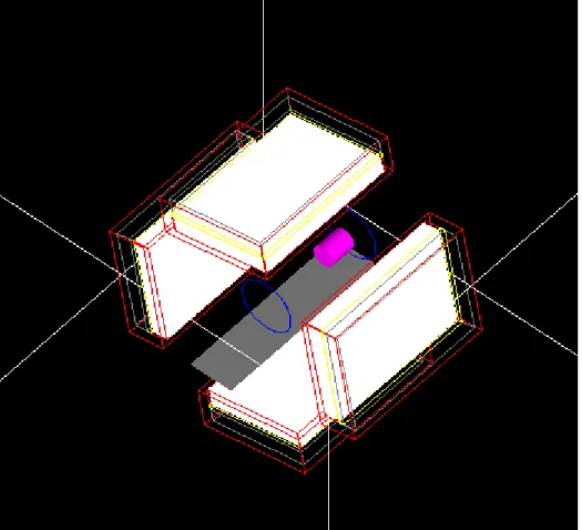
This benchmark simulates a SPECT procedure modeling a moving radioactive source.20 Much like the previous simulation, the gamma camera that is modeled does not correlate to any existing system but is rather an ideal simulated camera. An image generated with GATE depicting the system is shown in Figure 4.

(30)

19

Figure 4. Generated image of SPECT scan simulation

The SPECT scanner consists of four identical detector heads at 90 degree angles, each with 2 cm thick of lead shielding and 1 cm thick of NaI crystal. The NaI crystal is outlined yellow in Figure 4, and the magenta cylinder is a phantom of water 20 cm long and with a 2.5 cm radius. It contains a source cylinder filled with Tc-99m with a 1 cm radius and 5 cm long. The activity is set at 300 kBq. It also simulates the table, which is modeled to be 3 cm wide, 0.6 cm deep, and 34 cm long and shown in gray in Figure 4. The table, and thus source, translate in the Z plane at 0.04 cm per second. Since Tc-99m emits at 140 keV, only low energy electromagnetic interactions were processed. Furthermore,

(31)

20

secondary electrons were not tracked and x-rays were only tracked until their energy fell below the threshold of 20 keV. This allows for a sped up simulation without noticeably effecting results. It simulates a collection time of 600 seconds, with each head carrying out 16 projections. During this process the heads rotate in a circular manner at a speed of 0.15 degrees per second.

3.4.3 Gamma Beam Simulation

The Gamma Beam example is included as a sample simulation in GATE V6.1.21 It consists of a 5 meter cube of air, with a 40 cm cube water phantom within it. The cut-off energy is 0.1 keV. Incident on the water phantom is a circular 18 MeV gamma beam. Although the example originally simulates 2 million primary particles, it was increased to 20 million for this study. This increases the simulation runtime, which allows for a better time curve between cluster size and simulation time to be examined.

3.4.4 Radiotherapy Example

Version 6 of GATE added tools for radiation therapy applications. Several simulation frameworks are packaged with the GATE V6.1 installation to illustrate examples of its use for various photon and proton applications. From these, a radiotherapy example was chosen titled Novice_5.21_{This simulation was used due to its intuitive nature} and easy customizability. It simulates a proton beam in a water box with a Pencil Beam Scanning source. The water phantom is 40 cm x 40 cm in the transverse plane, and is only 1 nm thick. The pencil beam traces a pattern in the water box that originally spells out “GATE.” For a flair of school spirit, it was modified to spell out “UNLV.” While the original macro file simulates 10,000 primary particles, this number was increased to 1

(32)

21

million particles in order to enhance the counting statistics and reach an appreciably high run time for the simulation.

3.4.5 Proton beam on CT Image

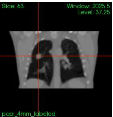
The final example used is the most complex and is available from the OpenGATE website.12 This simulation generates a 3D dose distribution of a proton spot beam incident on the CT image of a human chest. Unlike the other examples, which render a virtual representation of the simulation geometry, this simulation uses actual CT image data as input in generating the dose distribution. The CT image used in this case is called the POPI-model, which is an open source sample Thorax model from a real patient made available online for researchers.22 The CT has a clearly visible tumor in the right lung that can be used as the target for sample simulations such as this one, which is seen in the crosshairs in Figure 5. The image was downloaded as a DICOM image from their website and displayed using an image viewing and manipulating program called VV.23 VV is a cross platform and open-source medical image viewer. It was used to convert the image file from DICOM format to Analyze file format. This creates an .img file and .hdr header file that is compatible with GATE. This image is inserted into the macro file with a GATE command. In order to convert between HU and materials, a Density Table and Materials Table were downloaded from the open-source OpenGate Collaboration site.12 The proton beam simulated has a disk shape with a 6 mm diameter of 250 MeV energy.

(33)

22

(34)

23

CHAPTER 4 RESULTS

Each of the five simulations was repeated for all cluster sizes ranging from 1 to 20, and the time of simulation for each one recorded. In addition, the output of each run was saved. The PET and SPECT results were compared to the published benchmark data to verify compatibility and repeatability among all node sizes. Given the accuracy of the benchmark data and the fact that the others don’t have published results to compare them to, a side-by-side visual comparison was used to verify the consistency of the remaining three simulations.

(35)

24

Figure 6. Graphical output of PET Simulation on 15-node cluster

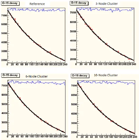
Figure 6 shows an example of the resulting output of a PET benchmark simulation. The results of each cluster size were compared and cross referenced with the expected values to verify that they were consistent with expected results. Figure 7 compares the decay vs time plot for 4 different node sizes as evidence of their consistencies. Given the stochastic nature of Monte Carlo simulations, the results are not expected to be identical. However, the counting statistics are high enough that the degree of variability should be low, and a glance of the side-by-side graphs in Figure 7 certainly suggests this.

(36)

25

Figure 7. Decay curves for various cluster sizes. F-18 activity is in blue and O-15 activity is in red. The O-15 decay curve fit is in black.

While the graphs give a good visual indication that the results are consistent, analyzing the numerical results allows for this to be proven statistically. The expected results of the PET Benchmark are published and available online to allow users to evaluate that their build of GATE is operating correctly.24 The values are found from averaging several repeat trials on different computer systems. The 4 main baseline values are random coincidences, unscattered coincidences, scattered coincidences, and O-15 lifetime. As seen in Table 1, the results closely matched the expectations of the benchmark across all cluster sizes, indicating that the cloud computing environment is not affecting the end result. The

(37)

26

following table summarizes this data, showing that all calculated values are within 1% of the expected, as mandated in the validation installation instructions.24_{There was one} exception to this while collecting data: the calculated half-life of Oxygen-15 for the 5-node cluster originally had 1.3% error. The simulation was run two additional times on a 5-node cluster, and the results were within 1%. This is the trial shown in the table. The initial run was considered an anomaly. The cause of this error was not determined, but was likely a node failure, an error in GATE itself, or simply random fluctuation.

These results give confidence that the size of the cluster does not affect the results of the simulation. Next, the relationship of cluster size and runtime of simulation was examined. Table 2 shows the runtime for each cluster size.

Table 1. PET output compared to expected benchmark data Cluster Size Random Coincidence % Error Unscattered Coincidence % Error Scattered Coincidence % Error O-15 Lifetime % Error Benchmark 23536 - 312725 - 370116 - 122.24 0.086 1 23499 0.157 312906 0.058 371144 0.278 122.26 0.020 2 23495 0.175 314235 0.483 370356 0.065 122.15 0.070 3 23439 0.411 311842 0.282 368864 0.338 122.27 0.024 4 23568 0.136 312828 0.033 370840 0.195 122.13 0.093 5 23527 0.036 311977 0.239 370859 0.201 122.15 0.072

(38)

27

Table 2. Runtime for each cluster size of PET benchmark

Nodes Time (min) Nodes Time (min) 1 204.47 11 16.52 2 83.76 12 13.16 3 59.58 13 12.67 4 41.80 14 12.21 5 31.95 15 10.70 6 28.10 16 10.17 7 27.51 17 9.86 8 23.47 18 9.03 9 20.01 19 8.74 10 16.30 20 7.79

These results show a falloff in computation time. A relationship between cluster size and simulation time was established, as seen in the Figure 8. Increasing the number of nodes in the cluster resulted in a decrease in calculation time that can be expressed with an exponential model. As one would expect, as the cluster size increased, there was a diminishing return in adding additional nodes.

6 23339 0.837 313173 0.143 370282 0.045 122.16 0.063 7 23674 0.585 314482 0.562 369567 0.148 122.28 0.029 8 23459 0.327 312851 0.040 370933 0.221 122.28 0.037 9 23571 0.150 313475 0.240 370226 0.030 122.17 0.055 10 23745 0.886 313608 0.282 369724 0.106 122.12 0.096 11 23528 0.036 312596 0.041 368112 0.541 122.24 0.003 12 23445 0.385 312895 0.054 369523 0.160 122.27 0.022 13 23587 0.217 313265 0.173 370116 0.000 122.38 0.113 14 23580 0.186 311262 0.468 370719 0.163 122.08 0.133 15 23556 0.086 312612 0.036 370093 0.006 122.33 0.073 16 23548 0.053 312247 0.153 370233 0.031 122.08 0.127 17 23563 0.114 312198 0.169 370177 0.016 122.37 0.109 18 23615 0.338 312276 0.144 370989 0.236 122.14 0.080 19 23586 0.214 314120 0.446 369812 0.082 122.32 0.063 20 23532 0.016 313554 0.265 370067 0.013 122.22 0.015

(39)

28

Figure 8. Graph of the relationship of cluster size and time of PET simulation

4.2 SPECT Benchmark

The output for the SPECT benchmark consisted solely of numerical values. The original benchmark had a relatively short runtime of around 40 minutes on a single node. Thus, the activity was increased from 30 kBq to 300 kBq. This increased the runtime on a single node to about 400 minutes, which allowed for a better look at simulation speedup from distributed computing. Unfortunately, this meant that some of the numerical results could no longer compared to the benchmark, such as detected counts or number of emitted particles. However, several other values were not affected by this because they are relative values. Thus, these are the output results used to assure the accuracy of the SPECT results.24 As seen in Table 3, this includes phantom scatter, table scatter, collimator scatter,

y = 189.58x-1.05 R² = 0.9952 0 50 100 150 200 250 0 2 4 6 8 10 12 14 16 18 20 Ti me in MInu tes Number of Nodes

(40)

29

and crystal scatter. Each of these values represents the percentage of photons whose last scattered event occurred in that specific medium.

Table 3. SPECT output compared to expected benchmark data Cluster Size Phantom Scatter % Error Table Scatter % Error Collimator Scatter % Error Crystal Scatter % Error Benchmark 53.300 0.0533 3.00 0.003 0.340 0.00986 6.70 0.0134 1 53.227 0.136 2.996 0.141 0.327 3.760 6.721 0.317 2 53.354 0.102 3.003 0.091 0.336 1.116 6.693 0.102 3 53.299 0.001 2.996 0.140 0.352 3.590 6.695 0.076 4 53.371 0.133 2.997 0.097 0.355 4.530 6.703 0.041 5 53.281 0.037 2.996 0.143 0.350 2.890 6.695 0.077 6 53.253 0.087 3.002 0.075 0.338 0.721 6.723 0.346 7 53.222 0.147 2.995 0.182 0.340 0.136 6.699 0.018 8 53.357 0.106 3.000 0.009 0.322 5.382 6.682 0.274 9 53.264 0.068 2.998 0.080 0.339 0.386 6.698 0.030 10 53.259 0.076 2.998 0.062 0.345 1.398 6.700 0.006 11 53.340 0.075 2.997 0.101 0.329 3.222 6.694 0.088 12 53.261 0.072 2.995 0.176 0.344 1.067 6.707 0.103 13 53.221 0.149 3.001 0.027 0.348 2.296 6.712 0.178 14 53.403 0.194 3.002 0.059 0.338 0.538 6.720 0.298 15 53.305 0.010 2.999 0.044 0.340 0.062 6.713 0.187 16 53.290 0.019 3.000 0.002 0.341 0.151 6.708 0.121 17 53.366 0.123 3.002 0.053 0.342 0.610 6.710 0.149 18 53.337 0.069 3.004 0.145 0.344 1.083 6.698 0.028 19 53.299 0.003 2.995 0.169 0.323 4.916 6.702 0.031 20 53.237 0.118 3.000 0.004 0.333 2.084 6.698 0.024

As the percent error in Table 3 shows, the error in each run of the simulation is much lower than the cut-off point of 1 percent. The exception to this is the collimator scatter. This value varies wildly due to its small scatter ratio and has a 2.4% standard deviation.20 This is likely due to the increase in activity from 30 kBq to 300 kBq. Not only did it increase the runtime but also increased the precision of the results. Table 4 shows

(41)

30

the runtime of this simulation on each cluster size. The runtime was 401.50 minutes on 1 node, and decreased to 16.48 minutes on 20 nodes.

Table 4. Runtime for each cluster size of SPECT benchmark

Nodes Time (min) Nodes Time (min)

1 401.50 11 31.24 2 199.20 12 28.48 3 133.30 13 26.19 4 87.60 14 24.22 5 71.98 15 22.49 6 59.96 16 21.51 7 50.78 17 19.71 8 42.36 18 18.54 9 38.80 19 17.39 10 34.67 20 16.48

Figure 9 shows a plot of the data in Table 4 along with an equation modeling the relationship. As predicted, it exhibits the same inverse power relationship as the others.

Figure 9. Graph of relationship between cluster size and time of SPECT simulation

y = 407.46x-1.07 R² = 0.9993 0 50 100 150 200 250 300 350 400 450 0 2 4 6 8 10 12 14 16 18 20 Ti me in Minu tes Number of Nodes

(42)

31

4.3 Gamma Beam Simulation

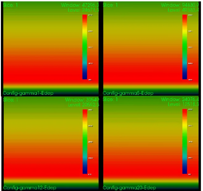
The output of the Gamma Beam Simulation shows the dose distribution of the incident beam of 18 MeV gamma beams on the water phantom. Examples of its output are shown for 1, 5, 12, and 20 node clusters in Figure 10. The gamma rays are incident on the phantom from the bottom of the picture. The build-up region can clearly be seen, followed by the depth of maximum dose and the falloff region. Results were identical across all cluster sizes. Thus, the cluster does not affect the integrity of result. The runtimes of the radiotherapy benchmark are shown below. The time of simulation was decreased from 243.85 minutes on 1 node down to 12.27 minutes on 20 nodes.

(43)

32

This decrease follows the same power relationship as the PET benchmark, only with different coefficients. Thus, as the cluster size increases there is a diminishing return on the investment of additional nodes. This can be seen in Table 5 and Figure 11.

Figure 10. Dose distribution output of the gamma beam. Top left is on 1 node, top right is 5 nodes, bottom left is 12 nodes, and bottom right is 20 nodes.

(44)

33

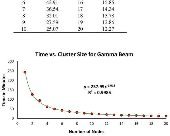
Table 5: Runtime for each cluster size of gamma simulation

1 243.85 11 23.10 2 126.30 12 20.73 3 94.57 13 18.95 4 61.85 14 17.49 5 49.97 15 16.77 6 42.91 16 15.85 7 36.54 17 14.34 8 32.01 18 13.78 9 27.59 19 12.86 10 25.07 20 12.27

Figure 11. Graph of the relationship of cluster size and time of gamma simulation

4.4 Radiotherapy Example

This example was successfully repeated on all cluster sizes from 1 node to 20 nodes. Across all cluster sizes the output appeared to be almost identical, with only a small level

y = 257.99x-1.013 R² = 0.9985 0 50 100 150 200 250 300 0 2 4 6 8 10 12 14 16 18 20 Ti me in Minu tes Number of Nodes

(45)

34

of visible variability as expected by Monte Carlo’s inherent randomness. Four examples of outputs are shown in Figures 12-15 for 1, 2, 5, and 15 node clusters respectively.

(46)

35

(47)

36

Figure 13. Output for Radiotherapy simulation on 2 nodes

(48)

37

Figure 15. Output for Radiotherapy simulation on 15 nodes

The following table shows the time of simulation for each cluster size. The time of simulation was sped up from 252.92 minutes on 1 node to 12.60 minutes on 20 nodes.

Table 6. Runtime for each cluster size of radiotherapy simulation

Node Time (min) Node Time (min)

1 252.92 11 22.01 2 119.10 12 20.43 3 85.86 13 19.21 4 61.30 14 17.80 5 52.33 15 16.71 6 41.96 16 14.78 7 36.30 17 14.20 8 32.10 18 13.64 9 26.96 19 12.97 10 24.61 20 12.60

(49)

38

This simulation follows a similar power-law speed-up as the others. The equation modeling this is shown in Figure 16.

Figure 16. Graph of the relationship of cluster size and time of radiotherapy simulation

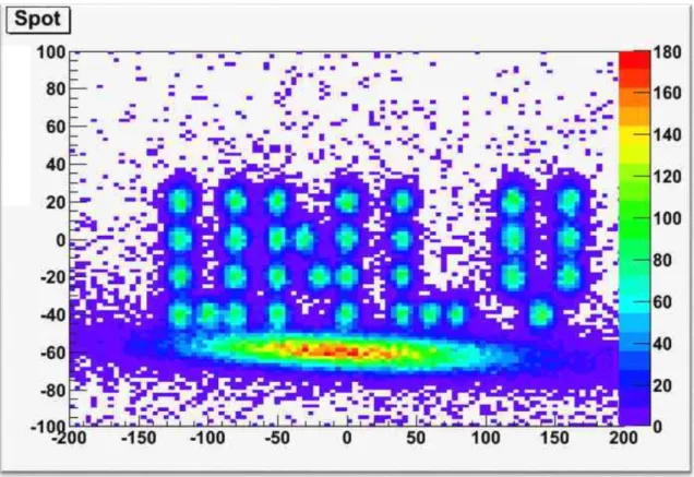
4.5 Proton Beam on CT Image

The simulation successfully imposed a dose calculation on the CT image, as shown in the figure below. It acts to serve as a proof-of-concept only, given that the treatment plan itself would be very poor at tissue sparing if actually used to treat the patient. The proton beam is incident from the transverse plane, as seen in Figure 17-19.

y = 252.58x

-1.008

R² = 0.999

0 50 100 150 200 250 300 0 2 4 6 8 10 12 14 16 18 20 Ti me in Minu tes Number of Nodes

(50)

39

Figure 17. Dose Distribution on 2 Node Cluster

(51)

40

Figure 19. Dose Distribution on 18 Node Cluster

VV allows for image viewing from different parts of the CT and different angles. Putting the output from all of the different cluster sizes into similar geometry showed that the output was roughly consistent among them. Examining the relationship of cluster size and time shows that that runtime of this simulation was decreased from 53 minutes on 1 machine to just 3.11 minutes on 20 machines. The results are shown in the below table.

Table 7. Runtime for each cluster size of proton beam simulation

1 53.00 11 5.15 2 27.25 12 4.67 3 18.83 13 4.51 4 13.63 14 4.18 5 11.53 15 4.02 6 9.48 16 3.74 7 8.49 17 3.53 8 7.21 18 3.25 9 6.32 19 3.20

(52)

41

10 5.62 20 3.11

This exhibits the same power-law decrease as the other simulations. It was plotted and a line of best fit found, as seen in Figure 20. As expected, it exhibits the same inverse power relationship as the others.

Figure 20. Graph of the relationship of cluster size and time of simulation

CHAPTER 5 DISCUSSION

Overall these are satisfying results; GATE simulations were successfully run in a commercial cloud computing environment while returning stable results. However, there

y = 52.892x-0.959 R² = 0.9991 0 10 20 30 40 50 60 0 2 4 6 8 10 12 14 16 18 20 Ti me in Minu tes Number of Nodes

(53)

42

were some inconsistencies that warranted additional examination. Assuming that a cluster has identical computers working at identical efficiency, one would expect a job taking X amount of time on one machine to take no less than X/N amount of time when distributed on N number of machines. This would be the theoretical limit for a truly parallel task, and in reality the time taken per node would be expected to be slightly more than X/N. However, in a few of these simulations the opposite was observed. The decrease in time actually exceeded that expected by an inverse power relationship. This implies that the assumption that the computers are identical and working at identical efficiency is not valid in this case. This could be due to inconsistent specs on the computers accessed from Amazon, changes in node compute speed based on workload, or quirks at the operational level in GATE functionality. The phenomena was not evident on all simulations, but was most prominent on the PET and SPECT Benchmarks. A thorough literature search did not uncover documentation of this phenomena for others, although in general there is scarce literature on GATE in a distributed environment. Figure 21 illustrates this phenomena by multiplying the runtime of each cluster size by the number of nodes in the cluster and graphing it. Ideally this would yield a straight flat line, or potentially a slight increase as cluster size increases.

(54)

43

Figure 21. Total cluster runtime for PET Benchmark

The runtime on a single node seemed to be the biggest outlier. By omitting this point from the graph in Figure 8 and remodeling the equation, the estimated time for a

one node cluster is 180 minutes. This can be seen in Figure 22.

Figure 22. Time vs. cluster size for PET Benchmark without outlier

To further examine this outlier, 4 repeat trials were carried out on one node, as shown in Table 8. Since repeat runs had different seeds, small variations in time is

y = 180x-1.028 R² = 0.9932 0 10 20 30 40 50 60 70 80 90 100 0 2 4 6 8 10 12 14 16 18 20 Ti me in MInu tes Number of Nodes

(55)

44

expected for the Monte Carlo simulation. However, if the calculation is repeated starting with the same random seed, then the exact same calculation is carried out and identical results should be expected. To test this, the fourth repeat was given the same random seed as the third. While the results were identical, the runtime varied by 7 minutes. This suggests that GATE software and/or EC2 is volatile in nature.

Table 8. PET Benchmark repeated on 1 node

Trial Seed Time

(mins)

1 Random 202 2 Random 216

3 Same 207

4 Same 214

Redundant simulations were carried out for other cluster sizes of the PET Benchmark in order to study the variation in time for repeat runs. Repeat runs were carried out for 1, 3, 5, 15, and 20 node cluster sizes. The time taken for the repeat runs is shown in Table 9 next to the time of the original runs. Variation in time was never more than a minute for cluster sizes larger than one.

Table 9. Time taken to run simulations under identical conditions

Nodes Run 1 Time (mins) Run 2 Time (mins) Run 3 Time (mins) 1 204.46 203.85 207.22 3 59.58 59.52 58.80 5 31.95 31.23 31.50 15 10.70 10.53 11.13 20 7.79 7.34 7.86

(56)

45

Amazon Web Services charges an hourly rate to use a given node, which is rounded up to the nearest hour. For the C1.medium nodes used in this study, the fee was $0.145/hr. Thus the total cost of running a simulation was determined by summing up the product of each node with its run time and $0.145/hr. Since for each node the run time is rounded up to the nearest hour, this causes an inflation of price for larger cluster sizes. This can be seen in the Table 10, which displays the cost to run the PET Benchmark simulation for each cluster size.

Table 10. Cost of cluster for PET Benchmark

No. of Nodes Cost ($) No. of Nodes Cost ($)

1 0.580 11 1.595 2 0.580 12 1.740 3 0.580 13 1.885 4 0.580 14 2.030 5 0.725 15 2.175 6 0.870 16 2.320 7 1.015 17 2.465 8 1.160 18 2.610 9 1.305 19 2.755 10 1.450 20 2.900

For a 15-node cluster, even though each individual node is only running for 15 minutes it is charged as a full hour. Thus, about 45 minutes of un-used time is paid for on each node. This could be a problem when running individual simulations, as costs add up. For each additional node added to the cluster, the speedup diminishes but the increase in cost remains the same. This means there is an optimal cluster size for a given simulation depending on the required speed and available funds. Past this point, the speed-up of

(57)

46

adding new nodes is offset by the increased price. Fortunately, this quirk in cost is only an issue when running single simulations on Amazon Web Services. In a hospital setting with a heavy load, instead of shutting down the cluster after a simulation is complete, the next simulation could immediately begin on the same cluster. This way there isn't un-used computer time that is paid for. Additionally, a different payment structure with AWS could be chosen. For this study, the pay-by-use hourly system was used. It is also possible to “rent” nodes for long-term use. Then they are owned for months or years and are always reserved for the user, and sit idle when not being used. This means that when they are needed, no waiting or slowdown from other AWS users will be experienced, which is something Amazon warns can happen using on-demand hourly use of nodes. If this is the case, when requests are sent to initialize nodes on EC2, a message is returned stating that none are currently available and an estimated wait time is given. This was never experienced over the course of this study. However, users are not explicitly warned of general slowdown in service due to high demand, so there was no obvious way to track if this occurred in this study. This could be a cause of the runtime outliers seen in the data. Ultimately this highlights a definite drawback of commercial cloud computing as a solution in that there are unknown and uncontrollable variables. Amazon puts great effort in making the technically complicated EC2 convenient and simple for the end-user, but this comes at the cost of knowing every detail of process.

Consistency is another important matter that would need to be addressed before hospital implementation. Amazon warns users that occasional node failures can happen, and during periods of high demand there can be wait-times before your cluster will initialize. As mentioned earlier, wait times and slowdowns were never experienced in this

(58)

47

study. However, occasional node failure did occur. A total of 5 times were detected where a node would either completely shut down or return incomplete results. In each case, a new node was launched and the same work sent to it. The results from the rest of the cluster would have to wait for the new node to finish before results could be combined. Despite the wait time it caused, this solution worked each of the five times a node failure was experienced.

Quality of internet access was not a controlled variable in this study. Internet speed was periodically measured using the online SpeedTest offered by Ookla.25 It ranged from the moderately quick download speed of 44.4 Mbps to a very poor 8.1 Mbps. Upload speed ranged from 35.4 Mbps to 6.1 Mbps. To avoid the extra variability the upload and download times would add to runtime, they were not included in the recorded time of simulations. However, given that upload and download speed is a relevant concern when discussing cloud computing, their effects on this study were still observed. The PET simulation required for only macro files to be uploaded, with a size on the order of 9 KB. However, the resulting root file was roughly 1.2 GB. Under optimal internet speed, the download took under a minute. In sub-optimal settings, it took up to 5 minutes. The SPECT simulation also required a macro file, but in addition needed to send a materials table to each node, which was only a few KBs in size. Both the Radiotherapy example and Gamma Beam example had a few materials tables uploaded in addition to their macro files, adding up to a rough total of 20 KBs. Thus even under the poorest internet connections experienced during this study, it never took more than 20 seconds to upload all necessary files to the cloud. They both had output files that were smaller than those of PET and SPECT, but still roughly 0.5 GBs. The simulation of a proton beam incident on a patient

(59)

48

was unique in that instead of just a macro file declaring the simulation geometry, an actual CT image was uploaded and used in the simulation. This meant that there was an upload file of non-negligible size as well. This most accurately reflects the scenarios encountered in a clinical setting, where patient CT data is needed in order to calculate dose distributions. The sum of all the files uploaded for this simulation was roughly 30 MB, taking anywhere between 10 seconds and a minute to upload, depending on internet speed. Overall this indicates that cloud computing of GATE is possible even with poor internet connections, but with an increased overall runtime as a penalty. Ideally, a high speed internet connection would be available at all times. This would be something any clinic interested in implementing cloud computing would want to address.

In order to implement cloud computing in a hospital, there are other issues that would need to be mitigated that were out of the scope of this proof-of-concept study. One such issue is being compliant with the Health Insurance Portability and Accountability Act of 1996 (HIPAA). Being HIPAA compliant is something hospitals are increasingly careful about, especially in an era of digital data. Opposed to having a local computing cluster, using cloud computing requires patient data leaving the hospital and being processed online. Even under very secure circumstances, this is something hospitals may be reluctant to practice. Amazon has recently announced they are working on making accessible nodes that are HIPAA compliant for use by government and hospitals that will be available in the future.26 The hospital would still need to take several steps on their end to meet HIPAA guidelines as well, such as encrypting data and separating patient information from the CT images that would need to be sent to the cloud.

(60)

49

If this work were to be continued, there are other variables that could be examined more thoroughly. Since this was primarily a proof-of-concept study, repeat trials were not rigorously performed. More redundant simulations could be carried out to get a better look at repeatability and reliability. Additionally, only the C1.medium instance was used to collect data, but there are several other instance types available. Running clusters on other instance sizes could give insight on the optimal computer specs and cost efficiency for running GATE in a cloud environment. Another future project would be to put together a graphic user interface to increase the ease of use. This would involve streamlining and automating every step of the process by combining the code created for this study with the pre-existing libraries and modules it builds off of. This would allow for a single user-friendly interface that could be downloaded by other GATE users for cloud computing so they can avoid the difficult and time-consuming process of implementing it themselves. Other future work would involve enhancing the program to be able to detect errors and node failures automatically. This would save the user from the burden of detecting errors themselves and would ideally catch errors that the user may miss. The program could also relaunch a node to replace any failures automatically so time isn’t lost doing so manually after a simulation is complete.

(61)

50

CHAPTER 6 CONCLUSION

A cloud computing framework was successfully created to run GATE Monte Carlo simulations for medical physics applications. Five different simulations were modeled, and each repeated for cluster sizes varying from 1 to 20. For each of them, the integrity of results was independent of cluster size. In addition, the relationship of cluster size and simulation runtime was found to be an inverse power relationship. While there were quirks in the consistency of runtime, EC2 was a nonvolatile environment in which to generate consistent results. Only 5 node failures were experienced over the entire course of the study, which translates to roughly 0.48%.

Overall this is a promising look into the future of the role of cloud computing in radiation treatment planning and medical physics in general. This work strongly suggests that clinically implemented Monte Carlo calculations can be sped up significantly and still be economically feasible. Meanwhile, GATE and other Monte Carlo codes continue to become more efficient and user-friendly. In addition, the economy of scale of Amazon’s expanding market has allowed them to lower prices for their EC2 service over time. As prices and availability of online computing resources continue to improve, it will look like a reasonable alternative to a local computer cluster. This leads one to conclude that clinical

(62)

51

implementation of Monte Carlo as the ‘gold standard’ of dose calculation will only become more attractive with time.

(63)

52

References:

[1] Rogers, D. W. (2006). Fifty years of Monte Carlo simulations for medical physics. Physics in Medicine and Biology, 51, 287-301.

[2] Bush, K., Gagne, I. M., Zavgorodni, S., Ansbacher, W., & Beckham, W. (2011). Dosimetric validation of Acuros XB with Monte Carlo methods for photon dose calculations. Medical Physics, 38, 2208-2221.

[3] Jan, S., Benoit, D., Becheva, E., Carlier, T., Cassol, F., Descourt, P., . . . Buvat, I. (2011). GATE V6: a major enhancement of the GATE simulation platform enabling modelling of CT and radiotherapy. Physics in Medicine and Biology, 56, 881-901. [4] Keyes, R. W., Romano, C., Arnold, D., & Luan, S. (2010). Radiation therapy

calculations using an on-demand virtual cluster via cloud computing. Medical Physics, http://arxiv.org/abs/1009.5282

[5] DeMarco, J. J., Solberg, T. D., & Chetty, I. (1999). Monte Carlo methods for dose calculation and treatment planning: a revolution for radiotherapy. Administrative Radiology Journal, 18, 24-27.

[6] Spezi, E., & Lewis, G. (2008). An overview of Monte Carlo treatment planning for radiotherapy. Radiation Protection Dosimetry, 131, 123-129.

[7] Kan, M. W., Cheung, J. Y., Leung, L. H., Lau, B. M., & Yu, P. K. (2011). The accuracy of dose calculations by anisotropic analytical algorithms for stereotactic radiotherapy in nasopharyngeal carcinoma. Physics in Medicine and Biology, 56, 397-413.

[8] Papadimitroulas, P., Loudos, G., Nikiforidis, G. C., & Kagadis, G. C. (2012). A dose point kernel database using GATE Monte Carlo simulation toolkit for nuclear

medicine applications: comparison with other Monte Carlo codes. Medical Physics, 39, 5238-5247.

[9] Pratx, G., & Xing, L. (2011). Monte Carlo simulation of photon migration in a cloud computing environment with MapReduce. Journal of Biomedical Optics, 16,

125003.

[10] Wang, H., Ma, Y., Pratx, G., & Xing, L. (2011). Toward real-time Monte Carlo simulation using a commercial cloud computing infrastructure. Physics in Medicine and Biology, 56, 175-181

[11] Na, Y. H., Suh, T. S., Kapp, D. S., & Xing, L. (2013). Toward a web-based real-time radiation treatment planning system in a cloud computing environment. Physics in Medicine and Biology, 58, 6525-6540.

[12] Sarrut, D., Pop, S., & Glatard, T. (2011). GateRT Practical Exercises. Retrieved from http://wiki.opengatecollaboration.org/index.php/GateRT-PracticalExercices-2011.