R E S E A R C H
Open Access
One-bit compressive sampling via
0
minimization
Lixin Shen
1,2*and Bruce W. Suter
2Abstract
The problem of 1-bit compressive sampling is addressed in this paper. We introduce an optimization model for reconstruction of sparse signals from 1-bit measurements. The model targets a solution that has the least0-norm
among all signals satisfying consistency constraints stemming from the 1-bit measurements. An algorithm for solving the model is developed. Convergence analysis of the algorithm is presented. Our approach is to obtain a sequence of optimization problems by successively approximating the0-norm and to solve resulting problems by exploiting the
proximity operator. We examine the performance of our proposed algorithm and compare it with the renormalized fixed point iteration (RFPI) (Boufounos and Baraniuk, 1-bit compressive sensing, 2008; Movahed et al., A robust RFPI-based 1-bit compressive sensing reconstruction algorithm, 2012), the generalized approximate message passing (GAMP) (Kamilov et al., IEEE Signal Process. Lett. 19(10):607–610, 2012), the linear programming (LP) (Plan and
Vershynin, Commun. Pure Appl. Math. 66:1275–1297, 2013), and the binary iterative hard thresholding (BIHT) (Jacques et al., IEEE Trans. Inf. Theory 59:2082–2102, 2013) state-of-the-art algorithms for 1-bit compressive sampling
reconstruction.
Keywords: 1-bit compressive sensing,1minimization,0minimization, Proximity operator
1 Introduction
Compressive sampling is a recent advance in signal acqui-sition [1, 2]. It provides a method to reconstruct a sparse signalx∈Rnfrom linear measurements
y=x, (1)
whereis a givenm×nmeasurement matrix withm<n and y ∈ Rm is the measurement vector acquired. The
objective of compressive sampling is to deliver an approx-imation toxfromyand. It has been demonstrated that the sparse signalxcan be recovered exactly fromyifhas Gaussian i.i.d. entries and satisfies the restricted isometry property [2]. Moreover, this sparse signal can be identi-fied as a vector that has the smallest0-norm among all vectors yielding the same measurement vectoryunder the measurement matrix.
However, the success of the reconstruction of this sparse signal is based on the assumption that the measurements have infinite bit precision. In realistic settings, the mea-surements are never exact and must be discretized prior
*Correspondence: [email protected]
1Department of Mathematics, Syracuse University, Syracuse, NY 13244, USA 2Air Force Research Laboratory. AFRL/RITB, Rome, NY 13441-4505, USA
to further signal analysis. In practice, these measurements are quantized, a mapping from a continuous real value to a discrete value over some finite range. As usual, quanti-zation inevitably introduces errors in measurements. The problem of estimating a sparse signal from a set of quan-tized measurements has been addressed in recent litera-ture. Surprisingly, it has been demonstrated theoretically and numerically that 1-bit per measurement is enough to retain information for sparse signal reconstruction. As pointed out in [3, 4], quantization to 1-bit measurements is appealing in practical applications. First, 1-bit quan-tizers are extremely inexpensive hardware devices that test values above or below zeros, enabling simple, effi-cient, and fast quantization. Second, 1-bit quantizers are robust to a number of non-linear distortions applied to measurements. Third, 1-bit quantizers do not suffer from dynamic range issues. Due to these attractive properties of 1-bit quantizers, in this paper, we will develop efficient algorithms for reconstruction of sparse signals from 1-bit measurements.
The 1-bit compressive sampling framework originally introduced in [3] is briefly described as follows. Formally, it can be written as
y=A(x):=sign(x), (2)
where the function sign(·) denotes the sign of the vari-able, element-wise, and zero values are assigned to be+1. Thus, the measurement operatorA, called a 1-bit scalar quantizer, is a mapping from Rn to the Boolean cube
{−1, 1}m. Note that the scale of the signal has been lost
during the quantization process. We search for a sparse signalxin the unit ball ofRmsuch that the sparse signal x is consistent with our knowledge about the signal and measurement process, i.e.,A(x)=A(x).
The problem of reconstructing a sparse signal from its 1-bit measurements is generally non-convex, and there-fore it is a challenge to develop an algorithm that can find a desired solution. Nevertheless, since this problem was introduced in [3] in 2008, there are several algorithms that have been developed for attacking it [3, 5–7]. Among those existing 1-bit compressive sampling algorithms, the binary iterative hard thresholding (BIHT) [4] exhibits its superior performance in both reconstruction error and as well as consistency via numerical simulations over the algorithms in [3, 5]. When there are a lot of sign flips in the measurements, a method based on adaptive outlier pur-suit for 1-bit compressive sampling was proposed in [7–9]. By formulating 1-bit compressive sampling problem in Bayesian terms, a generalized approximate message pass-ing (GAMP) [10] was developed to the problem of recon-struction from 1-bit measurements. The algorithms in [4, 7] require the sparsity of the desired signal to be given in advance. This requirement, however, is hardly satisfied in practice. By keeping only the sign of the measurements, the magnitude of the signal is lost. The models associated with the aforementioned algorithms seek sparse vectorsx satisfying consistency constraints (2) in the unit sphere. As a result, these models are essentially non-convex and non-smooth. In [6], a convex minimization problem is for-mulated for reconstruction of sparse signals from 1-bit measurements and is solved by linear programming. The details of the above algorithms will be briefly reviewed in the next section.
In this paper, we introduce a new 0 minimization model over a convex set determined by consistency con-straints for 1-bit compressive sampling recovery and develop an algorithm for solving the proposed model. Our model does not require prior knowledge on the sparsity of the signal. Our approach for dealing with our proposed model is to obtain a sequence of optimization problems by successively approximating the 0-norm and to solve resulting problems by exploiting the proximity operator [11]. Convergence analysis of our algorithm is presented.
This paper is organized as follows. In Section 2, we review and comment current 1-bit compressive sampling models and then introduce our own model by assimilat-ing advantages of existassimilat-ing models. Heuristics for solvassimilat-ing
the proposed model are discussed in Section 3. Conver-gence analysis of the algorithm for the model is studied in Section 4. A numerical implementable algorithm for the model is presented in Section 5. The performance of our algorithm is demonstrated and compared with the BIHT, RFPI, LP, and GAMP in Section 6. We present our conclusion in Section 7.
2 Models for one-bit compressive sampling In this section, we begin with reviewing existing models for reconstruction of sparse signals from 1-bit measure-ments. After analyzing these models, we propose our own model that assimilates the advantages of the existing ones. Using matrix notation, the 1-bit measurements in (2) can be equivalently expressed as
Yx≥0, (3)
whereY := diag(y)is anm×mdiagonal matrix whose ith diagonal element is theith entry ofy. The expression Yx ≥ 0 in (3) means that all entries of the vectorYx are no less than 0. Hence, we can treat the 1-bit mea-surements as sign constraints that should be enforced in the construction of the signalx of interest. In what fol-lows, Eq. (3) is referred to as sign constraint or consistency condition, interchangeably.
The optimization model for reconstruction of a sparse signal from 1-bit measurements in [3] is
minx1 s.t. Yx≥0 and x2=1, (4)
where · 1and · 2denote the1-norm and the2 -norm of a vector, respectively. In model (4), the1-norm objective function is used to favor sparse solutions, the sign constraintYx≥0 is used to impose the consistency between the 1-bit measurements and the solution, and the constraintx2=1 ensures a nontrivial solution lying on the unit2sphere.
Instead of solving model (4) directly, a relaxed version of model (4)
min
λx1+ m
i=1
h((Yx)i)
s.t. x2=1 (5)
was proposed in [3]. By employing a variation of the fixed point continuation algorithm in [12], an algorithm, which is called renormalized fixed point iteration (RFPI), was developed for solving model (5) efficiently. Here,λis a reg-ularization parameter andhis chosen to be the one-sided 1(or2) function, defined atz∈Ras follows
h(z):=
|z| or 12z2, ifz<0;
We remark that the one-sided2function was adopted in [3] due to its convexity and smoothness properties that are required by a fixed point continuation algorithm.
In [5], a restricted-step-shrinkage algorithm was pro-posed for solving model (4). This algorithm is similar in sprit to trust-region methods for nonconvex optimiza-tion on the unit sphere and has a provable convergence guarantees.
Binary iterative hard thresholding (BIHT) algorithms were recently introduced for reconstruction of sparse signals from 1-bit measurements in [4]. The BIHT algo-rithms are developed for solving the following constrained optimization model
min
m
i=1
h((Yx)i) s.t. x0≤s and x2=1,
(7)
where h is defined by Eq. (6), s is a positive integer, and the 0-norm x0 counts the number of non-zero entries inx. Minimizing the objective function of model (7) enforces the consistency condition (3). The BIHT algo-rithms for model (7) are a simple modification of the itera-tive thresholding algorithm proposed in [13]. It was shown numerically that the BIHT algorithms perform signifi-cantly better than the other aforementioned algorithms in [3, 5] in terms of both reconstruction error as well as consistency. Numerical experiments in [4] further show that the BIHT algorithm with hbeing the one-sided 1 function performs better in low noise scenarios while the BIHT algorithm withhbeing the one-sided2 function performs better in high noise scenarios. For the measure-ments having noise (i.e., sign flips), a robust method for recovering signals from 1-bit measurements using adap-tive outlier pursuit was proposed in [7], noise-adapadap-tive renormalized fixed point iterative (NARFPI) was intro-duced in [8], and noise-adaptive restricted step shrinkage (NARSS) was developed in [9].
The algorithms reviewed above for 1-bit compressive sampling are developed for optimization problems having convex objective functions and non-convex constraints. In [6], a convex optimization program for reconstruction of sparse signals from 1-bit measurements was introduced as follows:
minx1 s.t. Yx≥0 and x1=p, (8)
wherepis any fixed positive number. The first constraint Yx ≥ 0 requires that a solution to model (8) should be consistent with the 1-bit measurements. If a vectorx satisfies the first constraint, so isaxfor all 0 < a < 1. Hence, an algorithm for minimizing the1-norm by only requiring consistency with the measurements will yield the solutionxbeing zero. The second constraintx1= p is then used to prevent model (8) from returning a
zero solution, thus resolves the amplitude ambiguity. By taking the first constraint into consideration, we know that x1 = y,x; therefore, the second constraint becomesy,x =p. This confirms that both objective function and constraints of model (8) are convex. It was further pointed out in [6] that model (8) can be cast as a linear program. The corresponding algorithm is referred to as LP. As comparing model (8) with model (4), both the constraintx2 = 1 in model (4) and the constraint
x1=pin model (8), the only difference between both models, enforce a non-trivial solution. However, as we have already seen, model (8) with the constraintx1= pcan be solved by a computationally tractable algorithm.
Let us further comment on models (7) and (8). First, the sparsity constraint in model (7) is impractical since the sparsity of the underlying signal is unknown in gen-eral. Therefore, instead of imposing this sparse constraint, we consider to minimize an optimization model having the 0-norm as its objective function. Second, although model (8) can be tackled by efficient linear programming solvers and the solution of model (8) preserves the effec-tive sparsity of the underlying signal (see [6]), the solu-tion is not necessarily sparse in general as shown in our numerical experiments (see Section 6). Motivated by the aforementioned models and the associated algorithms, we plan in this paper to reconstruct sparse signals from 1-bit measurements via solving the following constrained optimization model
minx0 s.t. Yx≥0 and x1=p, (9)
wherepis again an arbitrary positive number. This model has the 0-norm as its objective function and inequal-ity Yx ≥ 0 and equality x1 = p as its convex constraints.
We remark that the actual value ofpis not important as long as it is positive. More precisely, suppose thatS and
S are two sets collecting all solutions of model (9) with p = 1 andp = p > 0, respectively. If x ∈ S, that is, Yx ≥ 0 andx1 = 1, then, by denotingx := p x, it can be verified that x 0 = x0, Yx ≥ 0, and
x 1=p . That indicatesx ∈S . Therefore, we have thatp S ⊂ S . Conversely, we can show thatS ⊂ p S by reverting above steps. Hence,p S =S . Without loss of generality, the positive numberpis always assumed to be 1 in the rest part of the paper.
We compare model (7) and our proposed model (9) in the following result.
x
x2 as its solution ifx0 ≤ s; otherwise, model (7) can
not have a solution satisfying the consistency constraint if
x0>s.
Proof. Since the vectorxis a solution to model (9), then xsatisfies the consistency constraintYx≥ 0. Hence, it, together with definition ofhin (6), implies that
m model (7) do not satisfy the consistency constraint. Sup-pose this statement isfalse. That is, there exists a solution of model (7), sayx, such thatYx ≥ 0,x0 ≤ s, and turns out thatxis not a solution of model (9). This contra-dicts our assumption on the vectorx. This completes the proof of the result.
From Proposition 1, we can see that the sparsitysfor model (7) is critical. If s is set too large, a solution to model (7) may not be the sparsest solution satisfying the consistency constraint; ifsis set too small, solutions to model (7) cannot satisfy the consistency constraint. In contrast, our model (9) does not require the sparsity constraint used in model (7) and delivers the sparsest solution satisfying the consistency constraint. Therefore, these properties make our model more attractive for 1-bit compressive sampling than the BIHT.
To close this section, we recall an algorithm in [10] for the recovery of signals based on generalized approx-imate message passing (GAMP). This algorithm exploits the prior statistical information on the signal for esti-mating the minimum-mean-squared error solution from 1-bit measurements. The performance of GAMP will be included in our numerical section.
3 An algorithm for 1-bit compressive sampling In this section, we will develop algorithms for the pro-posed model (9). We first reformulate model (9) as an unconstrained optimization problem via the indicator function of a closed convex set in Rm+1. It turns out that the objective function of this unconstrained opti-mization problem is the sum of the 0-norm and the indicator function composing with a matrix associated with the 1-bit measurements. Instead of directly solving the unconstrained optimization problem, we use some smooth concave functions to approximate the 0-norm
and then linearize the concave functions. The result-ing model can be viewed as an optimization problem of minimizing a weighted1-norm over the closed con-vex set. The solution of this resulting model is served as a new point at which the concave functions will be linearized. This process is repeatedly performed until a certain stopping criterion is met. Several concrete exam-ples for approximating the0-norm are provided at the end of this section.
We begin with introducing our notation and recall-ing some background from convex analysis. For the d -dimensional Euclidean space Rd, the class of all lower semicontinuous convex functionsf : Rd → (−∞,+∞]
Next, we reformulate model (9) as an unconstrained optimization problem. To this end, from them×nmatrix and them-dimensional vectoryin Eq. (2), we define an (m+1)×nmatrix
respectively. Then, a vectorxsatisfies the two constraints of model (9) if and only if the vectorBxlies in the setC. Hence, model (9) can be rewritten as
min{x0+ιC(Bx):x∈Rn}. (12)
Problem (12) is known to be NP-complete due to the non-convexity of the 0-norm. Thus, there is a need for an algorithm that can pick the sparsest vectorxsatisfying the relationBx ∈ C. To attack this0-norm optimization problem, a common approach that appeared in recent lit-erature is to approximate the0-norm by its computation-ally feasible approximations. In the context of compressed sensing, we review several popular choices for defining the 0-norm as the limit of a sequence. More precisely, for a positive number ∈(0, 1), we consider separable concave functions of the form
where f : R+ → Ris strictly increasing, concave, and twice continuously differentiable such that
lim
→0+F (x)= x0, for all x∈R
The parameter plays a role of determining the quality of the approximationF (x)tox0. Since the functionf is concave and smooth onR+:=[ 0,∞), it can be majorized by a simple function formed by its first-order Taylor series expansion at a arbitrary point. WriteF (x,v) := F (v)+ is the absolute value of the corresponding element ofu. Clearly, whenvis close enough tox,F (x,v)the expres-sion on the right-hand side of (15) provides a reasonable approximation to the one on its left-hand side. Therefore, it is considered as a computationally feasible approxima-tion to the 0-norm of x. With such an approximation, a simplified problem is solved and its solution is used to formulate another simplified problem which is closer to the ideal problem (12). This process is then repeated until the solutions to the simplified problems become sta-tionary or meet a termination criteria. This procedure is summarized in Algorithm 1.
Algorithm 1(Iterative scheme for model (12))
Initialization: choose ∈(0, 1)and letx(0)∈Rnbe an
untila given stopping criteria is met
The termsF (|x(k)|)and∇F (|x(k)|),|x(k)|that appear
in the optimization problem in Algorithm 1 can be ignored because they are irrelevant to the optimization problem. Hence, the expression forx(k+1)in Algorithm 1 can be simplified as
x(k+1)∈argmin∇F (|x(k)|),|x| +ιC(Bx):x∈Rn.
(16)
Since f is strictly concave and increasing on R+, f is positive on R+. Hence, ∇F (|x(k)|),|x| = tive function of the above optimization problem is convex. Details for finding a solution to the problem will be pre-sented in the next section.
In the rest of this section, we list two possible choices of the functions in (13), namely, the Mangasarian function in
[14] and the Log-Det function in [15]. Many other choices can be found from [16–21] and the references therein.
The Mangasarian function is given as follows:
F (x)=
wherex ∈ Rn. This function is used to approximate the 0-norm to obtain minimum-support solutions (that is, solutions with as many components equal to zero as pos-sible). The usefulness of the Mangasarian function was demonstrated in finding sparse solutions of underdeter-mined linear systems (see [22]).
The Log-Det function is defined as
F (x)= named as the Log-Det heuristic and used for minimizing the rank of a positive semidefinite matrix over a convex set in [15]. Constant terms can be ignored since they will not affect the solution of the optimization problem (16). Hence, the Log-Det function in (18) can be replaced by
F (x)= n
i=1
log(|xi| + ). (19)
We point it out that the Mangasarian function is bounded by 1; therefore, it is non-coercive while the Log-Det function is coercive. This makes a difference in convergence analysis of the associated Algorithm 1 that will be presented in the next section. In what follows, the functionF is the Mangasarian function or the Log-Det function. We specify it only when it is noted.
4 Convergence analysis
In this section, we shall give convergence analysis for Algorithm 1. We begin with presenting the following result.
Theorem 2.Given ∈ (0, 1), x(0) ∈ Rn, and the setC defined by (11), let the sequence{x(k):k∈N}be generated by Algorithm 1, whereNis the set of all natural numbers. Then the following three statements hold:
(i) The sequence{F (x(k)):k∈N}converges whenF is corresponding to the Mangasarian function (17) or the Log-Det function (19);
(ii) The sequence{x(k):k∈N}is bounded whenF is the Log-Det function;
Proof. We first prove item (i). The key step for proving it is to show that the sequence{F (x(k)):k∈N}is decreas-ing and bounded below. The boundedness of the sequence is due to the fact that F (0) ≤ F (x(k)). From Step 1 of Algorithm 1 or Eq. (16), one can immediately have that
ιC(Bx(k+1))=0 ing and bounded below. Item (i) follows immediately.
WhenF is chosen as the Log-Det function, the coer-civeness of F together with item (i) implies that the sequence{x(k) :k∈N}must be bounded, that is, item (ii)
where v is some point in the line segment linking the points|x(k+1)|and|x(k)|and∇2F (v)is the Hessian matrix ofF at the pointv.
By (20), the first term on the right hand of Eq. (21) is less thanF (x(k)). By Eq. (19),∇2F (v)forvlying in the first octant of Rn is a diagonal matrix and is equal to −1
Mangasarian or the Log-Det function. Hence, the matrix ∇2F (v)is negative definite. Since the sequence{x(k):k∈
N}is bounded, there exists a constantρ >0 such that (w(k))∇2F (v)w(k)≤ −ρw(k)22.
Putting all above results together into (21), we have that
F (x(k+1))≤F (x(k))−ρ 2
|x(k+1)| − |x(k)|2 2.
Summing the above inequality fromk = 1 to+∞and using item (i) we get the proof of item (iii).
From item (iii) of Theorem 2, we have
|x(k+1)| − |x(k)|
2→0 ask→ ∞.
To further study properties of the sequence{x(k) : k ∈
N}generated by Algorithm 1, the matrix Bis required to have the range space property (RSP) which is originally introduced in [23]. With this property and motivated by the work in [23], we prove that Algorithm 1 can yield a sparse solution for model (12).
Prior to presenting the definition of the RSP, we intro-duce the notation to be used throughout the rest of this paper. Given a setS⊂ {1, 2,. . .,n}, the symbol|S|denotes the cardinality ofS, andSc:= {1, 2,. . .,n}\Sis the comple-ment ofS. Recall that for a vectoru, by abuse of notation, we also use|u|to denote the vector whose elements are the absolute values of the corresponding elements ofu. For a given matrix A having n columns, a vector u in Rn, and a setS ⊂ {1, 2,. . .,n}, we use the notation A
S
to denote the submatrix extracted fromA with column indices inSanduS the subvector extracted fromuwith
component indices inS.
Definition 3(Range space property (RSP)).Let A be an m×n matrix. Its transpose A is said to satisfy the range space property (RSP)of order K with a constantρ > 0if for all sets S⊆ {1,. . .,n}with|S| ≥K and for allξ in the range space of Athe following inequality holds
ξSc1≤ρξS1.
The range space property states that the range of the matrixAcontains no vectors where some entries have a significantly larger magnitude with respect to the oth-ers. We remark that if the transpose of anm×nmatrix Ahas the RSP of order K with a constant ρ > 0, then for every non-empty setS ⊆ {1,. . .,n}, the transpose of the matrix AS, denoted by AS, has the RSP of orderK
with constantρas well. We further remark that there is a relationship (see Proposition 3.6 in [23]) between the RSP and the restricted isometry property (RIP) and null space property (NSP) ofAwhich have been widely used in the compressive sensing literature. For example, if we have a matrix satisfying the NSP or RIP, we may construct a matrix satisfying the RSP. Unfortunately, similar to the RIP and the NSP, the RSP is hard to verify in practice.
The next result shows that if the transpose of the matrix Bin Algorithm 1 possesses the RSP, then Algorithm 1 can lead to a sparse solution for model (12). To this end, we define a mappingσ : Rd → Rd such that theith com-ponent of the vectorσ(u)is theith largest component of |u|.
Proposition 4. Let B be the(m+1)×n matrix be defined by (10) and let{x(k) : k ∈ N}be the sequence generated by Algorithm 1. Assume that the matrix Bhas the RSP of order K withρ >0satisfying(1+ρ)K <n. Suppose that the sequence{x(k) : k ∈ N}is bounded. Then,(σ(x(k)))
n the nth largest component of x(k)converges to 0.
Proof. Suppose this proposition isfalse. Then there exist a constantγ > 0 and a subsequence{x(kj) : j∈ N}such that(σ(x(kj)))
n ≥2γ > 0 for allj∈ N. From item (iii) of
(σ(x(kj+1))) for all sufficient largej. In what follows, we assume that the integerjis large enough such that the above inequalities in (23) hold.
Since the vector x(kj+1) is obtained through step 1 of Algorithm 1, i.e., Eq. (16), then by Fermat’s rule and the chain rule of subdifferential, we have that
0=diag(y(kj))∂ ·
1(diag(y(kj))x(kj+1))+Bb(kj+1),
whereb(kj+1)∈∂ι
C(Bx(kj+1)). By (23), we get
∂ · 1(diag(y(kj))x(kj+1))= {sgn(x(kj+1))},
where sgn(·)denotes the sign of the variable element-wise. Thus
y(kj)= |ξ(kj+1)|,
whereξ(kj+1)=Bb(kj+1)is in the range ofB.
Let S be the set of indices corresponding to the K smallest components of|ξ(kj+1)|. Hence,
However, by the definition ofσ, we have that
n−K
These inequalities together with the condition (1 + ρ)K<nlead to
which contradicts to (24). This completes the proof of the proposition.
From Proposition 4, we conclude that a sparse solution is guaranteed via Algorithm 1 if the transpose ofB satis-fies the RSP. Next, we answer how sparse this solution will be. To this end, we introduce some notation and develop a technical lemma. For a vector x ∈ Rd, we denote by (10), let F be the Log-Det function defined by (19), and let
{x(k) : k ∈ N}be the sequence generated by Algorithm 1. Assume that the matrix Bhas the RSP of order K with
ρ > 0 satisfying(1+ρ)K < n. If there existμ > ρ n to the optimization problem (16), then by Fermat’s rule and the chain rule of subdifferential we have that
However, since i0 is not in the set Iμ(x(k)) and B
satisfies the RSP, we have that
|(Bb(k+1))i0| ≤
i∈/Iμ(x(k))
|(Bb(k+1))i|
≤ ρ
i∈Iμ(x(k))
|(Bb(k+1))i| ≤ρW∗,
which contradicts to (25). Hence, we have thatx(i0k+1)=0 and|τ(x(k+1))|<n. By replacingkbyk+1 and repeat-ing this process, we can obtainx(i0k+) = 0 for all∈ N. Therefore,x0 < nfor allk > k. This process can be also applied to other components satisfyingx(ik+1) = 0. Thus there exists ak∈Nsuch thatτ(x(k))⊆τ(x(k))for allk≥k.
With Lemma 5, the next result shows that when the transpose ofBsatisfies the RSP, there exists a cluster point of the sequence generated by Algorithm 1 that is sparse and satisfies the consistency condition.
Theorem 6. Let B be the(m+1)×n matrix defined by (10), let F be the Log-Det function defined by (19), and let{x(k) : k ∈ N}be the sequence generated by Algorithm 1. Assume that the matrix Bhas the RSP of order K with
ρ > 0 satisfying(1+ρ)K < n. Then, there is a subse-quence{x(kj):j∈N}that converges to a(1+ρ)K-sparse solution, that is(σ(x(kj)))
(1+ρ)K+1→0as j→ +∞and
→0.
Proof. Suppose the theorem is false. Then, there exist μ∗, for any 0< ∗ < μ∗
ρn, there exist a ∈ (0, ∗)andk
such that(σ(x(k)))(1+ρ)K+1≥μ∗for allk≥k. It implies that for allk≥k
|Iμ∗(x(k))| ≥ (1+ρ)K+1> (1+ρ)K>K. (26)
By Lemma 5, there exist ak≥ksuch thatx(k) 0<n andτ(x(k+1)) ⊆ τ(x(k))for allk ≥k. LetS = τ(x(k)).
Thusx(Skc) = 0 for allk ≥k. Therefore, the optimization problem (16) for updating x(k+1) can be reduced to the following one
xkS+1∈arg min{(∇F (|x(k)|))S,u+ι((BS)u):u∈R|S|}.
(27)
If |τ(x(k))| > |Iμ∗(x(k))|, from (26), we have (1 + ρ)K<|S|. Thus, from Lemma 5 andBS having RSP with the same parameters, there exist a k > k such that
τ(x(k)) < τ(x(k))for allk≥k. Therefore, by induction,
there must exist ak˜such that for allk≥ ˜k
τ(x(k))=Iμ∗(x(k)), τ(xk)⊆τ(x(k˜)).
It means that for allk≥ ˜k, all the nonzero components ofx(k)are bounded below byμ∗. Therefore, for anyk≥ ˜k, the updating Eq. (16) is reduced by (27) withS=Iμ∗(x(k)).
From Lemma 4, we get [σ(x(k))]
|S|→0 which contradicts with|xk|S|| ≥μ∗. Therefore, we get this theorem.
5 An implementation of Algorithm 1
In this section, we describe in detail an implementation of Algorithm 1 and show how to select the parameters of the associated algorithm.
Solving problem (16) is the main issue for Algorithm 1. A general model related to (16) is
min{x1+ϕ(Bx):x∈Rn}, (28)
where is a diagonal matrix with positive diagonal ele-ments andϕ is in0(Rm+1). In particular, if we choose
= ∇F (|x(k)|)andϕ=ι
C, wherex(k)is a vector inRn,
is a positive number,Cis given by (11), andF is a function given by (13), then model (28) reduces to the optimization problem in Algorithm 1.
We solve model (28) by using recently developed first-order primal-dual algorithm (see, e.g., [24–26]). To present this algorithm, we need two concepts in con-vex analysis, namely, the proximity operator and conju-gate function. The proximity operator was introduced in [27]. For a function f ∈ 0(Rd), the proximity oper-ator of f with parameter λ, denoted by proxλf, is a mapping from Rd to itself, defined for a given point x∈Rdby
proxλf(x):=argmin
1
2λu−x 2
2+f(u):u∈Rd
.
The conjugate off ∈0(Rd)is the functionf∗∈0(Rd) defined atz∈Rdby
f∗(z):=sup{x,z −f(x):x∈Rd}.
Algorithm 2PD subroutine (the first-order primal-dual algorithm for solving (28))
Input: the(m+1)×nmatrixBdefined by (10); two positive numbersαandβsatisfying the relationαβ <
1
B2; the n×n diagonal matrix with all diagonal
elements positive; and the functionϕ∈0(Rn). Initialization: i = 0 and an initial guess (u(−1),u(0),x(0))∈Rm+1×Rm+1×Rn
repeat(i≥0)
Step 1: Computex(i+1):
x(i+1)=proxα·1◦
x(i)−αB(2u(i)−u(i−1))
Step 2: Computeu(i+1):
u(i+1)=proxβϕ∗(u(i)+βBx(i+1))
Step 3: Seti:=i+1.
untila given stopping criteria is met and the corre-sponding vectorsu(i),u(i+1), andx(i+1)are denoted by ucur,unew, andxnew, respectively.
Output: (ucur,unew,xnew) =
PD(α,β,B,,ϕ,u(−1),u(0),x(0))
Theorem 7.Let B be an(m+1)×n matrix defined by (10), letCbe the set given by (11), letαandβbe two positive numbers, and let L be a positive such that L≥ B2, where
Bis the largest singular value of B. If
αβL<1,
then for any arbitrary initial vector(x−1,x0,u0) ∈ Rn×
Rn × Rm+1, the sequence {xk : k ∈ N} generated by Algorithm 2 converges to a solution of model (28).
The proof of Theorem 7 follows immediately from Theorem 1 in [24] or Theorem 3.5 in [25]. We skip its proof here.
Both proximity operators proxα·1◦ and proxβϕ∗
should be computed easily and efficiently in order to make the iterative scheme in Algorithm 2 numerically efficient. Indeed, the proximity operator proxα·1◦is given atz∈
Rnas follows: forj=1, 2,. . .,n
proxα·1◦(z)j=max|zj| −αγj, 0·sign(zj), (29)
whereγjis thejth diagonal element of. Using the
well-known Moreau decomposition (see, e.g., [27, 28])
proxβϕ∗=I−βprox1
βϕ◦
1
βI , (30)
we can compute the proximity operator proxβϕ∗ via
prox1
βϕ which depends on a particular form of the func-tionϕ. As our purpose is to develop algorithms for the
optimization problem in Algorithm 1, we need to com-pute the proximity operator ofι∗C which is given in the following.
Lemma 8. IfCis the set given by (11) andβis a positive number, then for z∈Rm+1, we have that
proxβι∗
C(z)=(z1−(z1)+,. . .,zm−(zm)+,zm+1−β),
(31)
where(s)+is s if s≥0and 0 otherwise.
Proof.We first give an explicit form for the proximity operator prox1
βιC. Note that ιC =
1
βιC forβ > 0 and
ιC(z)=ι{1}(zm+1)+im=1ι[0,∞)(zi), forz∈Rm+1. Hence,
we have that
prox1
βιC(z)=((z1)+,(z2)+,. . .,(zm)+, 1), (32)
where(s)+issifs≥ 0 and 0 otherwise. Here we use the facts that proxι
[0,+∞)(s)=(s)+and proxι{1}(s)= 1 for any
s∈R.
By the Moreau decomposition (30), we have that proxβι∗
C(z) = z − βproxβ1ιC(
1
βz). This together with
Eq. (32) yields (31).
Next, we comment on the diagonal matrix in
model (28). When the functionϕin model (28) is chosen to beιC, then the relation aϕ = ϕ holds for any
posi-tive numbera. Hence, by rescaling the diagonal matrix in model (28) with any positive number, the solutions of model (28) are not altered. Therefore, we can assume that the largest diagonal entry ofis always equal to one.
In applications of Theorem 7 as in Algorithm 2, we should make the product ofαandβas close to 1/B2as possible. In our numerical simulations, we always set
α= β0.999
B2. (33)
In such a way,β is essentially the only parameter that needs to be determined.
Prior to computingαfor a givenβby Eq. (33), we need to know the norm of the matrix B. When min{m,n} is small, the norm of the matrixBcan be computed directly. When min{m,n} is large, an upper bound of the norm of the matrixBis estimated in terms of the size ofBas follows.
Proposition 9. Let be an m× n matrix with i.i.d. standard Gaussian entries and y be an m-dimensional vector with its component being+1 or−1. We define an
(m+1)×n matrix B fromand y via Eq. (10). Then,
Moreover,
B ≤√m+1(√n+√m+t)
holds with probability at least1−2e−t2/2for all t≥0. Proof. By the structure of the matrixBin (10), we know that
Therefore, we just need to compute the norms on the right-hand side of the above inequality. Denote byIm the m × m identity matrix and 1m the vector with all its
components being 1. Then,
which is a special arrow-head matrix and hasm+1 as its largest eigenvalue (see [29]). Hence,
diag(y) y
=√m+1.
Furthermore, by using random matrix theory for the
matrix, we know thatE{} ≤√n+√mand ≤
√
n+√m+twith probability at least 1−2e−t2/2for all t ≥ 0 (see, e.g., [30]). This completes the proof of this proposition.
Let us compute the norm of B numerically for 100 randomly generated matrices and vectors y for the pair (m,n) with three different choices (500, 1000), (1000, 1000), and(1500, 1000), respectively. Correspond-ing to these choices, the mean values ofBare about 815, 1276, and 1711 while the upper bounds of the expected values ofBby Proposition 9 are about 1208, 2001, and 2726, respectively. We can see that the norm ofBvaries with its size and turns to be a big number when the value of min{m,n} is relatively large. As a consequence, the parameterαorβmust be very small relative to the other by Eq. (33). Therefore, in what follows, the used matrixB in model (28) is considered to have been rescaled in the following way:
when the norm ofBcan be computed easily or not. The complete procedure for model (12) and how the PD subroutine is employed are summarized in Algorithm 3.
Algorithm 3(Iterative scheme for model (12))
Input: the(m+1)×nmatrixBformed by anm×n matrixand anm-dimensional vectoryvia (10); the setCgiven by (11); ∈(0, 1), andτ >0;αmaxand min be two real numbers; the maximum iteration number kmax.
Initialization: normalizing B according to (34); being the n × n identity matrix; an initial guess (uold0,ucur0,x(0)) ∈ Rm+1× Rm+1×Rn; and initial
Step 2: Update as the scaled matrix
diag(∇F (x(k+1))) such that the largest diagonal
In this section, we demonstrate the performance of Algo-rithm 3 for 1-bit compressive sampling reconstruction in terms of accuracy and consistency and compare it with the BIHT, RFPI, LP, and GAMP.
(a)
(b)
refers to the number of nonzero coefficients that are “misidentified,” i.e., coefficients that are determined to be nonzero when they should be zero. The last two metrics measure how well each algorithm finds the signal sup-port, meaning the locations of the nonzero coefficients. A higher value of SNR indicates a better reconstructed signal. The smaller the values of the rest three metrics are the better the reconstructed signals will be. The accu-racy of all test algorithms is measured by the average of values of these four metrics over 100 trials unless oth-erwise noted. For all figures in this section, results by the BIHT, RFPI, LP, GAMP, and Algorithm 3 with the Mangasarian function (17) and the Log-Det function (19) are marked by the symbols “,” “,” “,” “,” “◦,” and “,” respectively.
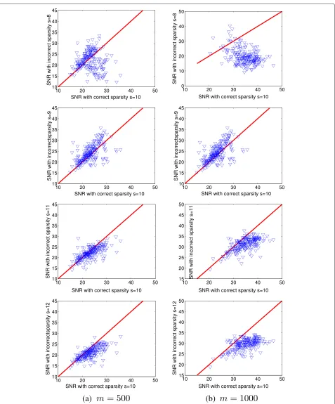
6.1 Effects of using inaccurate sparsity on the BIHT The BIHT requires knowing the sparsity of the underly-ing signals. This requirement is, however, not known in practical applications. In this subsection, we demonstrate through numerical experiments that the mismatched sparsity for a signal will degenerate the performance of the BIHT.
To this end, we fix n = 1000 and s = 10 and con-sider two cases ofmbeing 500 and 1000. For each case, we vary the sparsity input for the BIHT from 8 to 12 in which 10 is the only right choice. Therefore, there are total ten configurations. For each configuration, we record the SNR values of the reconstructed signals by the BIHT.
Figure 1 depicts the SNR values of the experiments. The plots in the left column of Fig. 1 are for the case
(a)
(b)
(c)
(d)
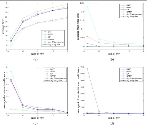
Fig. 2Algorithm comparison with configuration 1 for fixedn=1000 ands=10.aaverage SNR vsm/n;baverage Hamming error vsm/n;c
m = 500 while the plots in the right column are for the case m = 1000. The marks in each plot represent the pairs of the SNR values with the correct sparsity input (i.e.,s = 10) and with a mismatched sparsity input (i.e., s = 8, s = 9, s = 11, or s = 12 corresponding to the row 1, 2, 3, or 4). A mark below the red line indi-cates that the BIHT with the correct sparsity input works better than the one with an incorrect sparsity input. A mark that is far away from the red line indicates the BIHT with the correct sparsity input works much bet-ter than the one with an incorrect sparsity input or vice versa. Except the second plot in the left column, we can see that the BIHT with the correct sparsity input performs better than the one with an inaccurate spar-sity input. In particular, when an underestimated sparspar-sity
input to the BIHT is used, the performance of the BIHT will be significantly reduced (see the plots in the first two columns of Fig. 1). When an overestimated spar-sity input to the BIHT is used, majority of the marks are under the red lines and are relatively closer to the red lines than those from the BIHT with underestimated sparsity input. We further report that the average SNR values for the sparsity input s = 8, 9, 10, 11, and 12 form = 500 are 21.89, 24.18, 23.25, 22.10, and 21.00dB, respectively. Similarly, for m = 1000, the average SNR values for the sparsity input s = 8, 9, 10, 11, and 12 are 19.77dB, 26.37dB, 34.74dB, 31.12dB, and 29.46dB, respectively. In summary, we conclude that a proper cho-sen sparsity constraint is critical for the success of the BIHT.
(a)
(b)
(c)
(d)
6.2 Performance of Algorithm 3
Prior to applying Algorithm 3 for 1-bit compressive sam-pling problem, parameterskmax, τ, αmax, min, α, and in Algorithm 3 need to be determined. Under the afore-mentioned setting for the random matrix and sparse signalx, we fixkmax = 13,τ = 12,αmax = 8000, min = 10−4. For the functions F defined by (17) and (19), we set the pair of initial parameters(α, )as(500, 0.25)and (250, 0.125), respectively. The iterative process in the PD subroutine is forced to stop if the corresponding number of iteration exceeds 300. These parameters are used in all simulations performed by Algorithm 3 in the rest of this section.
To evaluate the performance of Algorithm 3 at vari-ous scenarios, the following three configurations fornthe
dimension of the signal,mthe number of measurements, andsthe sparsity of the vectorx, are considered:
• configuration 1:n=1000,s=10, and m=100, 500, 1000, 1500
• configuration 2:m=1000,n=1000, and s=5, 10, 15, 20
• configuration 3:m=1000,s=10, and n=500, 800, 1200, 1400
For every case in each configuration, we compare the accuracy of Algorithm 3 with the BIHT, RFPI, LP, and GAMP by computing the average of values of the four metrics over 100 trials. We remark that Algorithm 3, RFPI, LP, and GAMP do not require the knowledge of sparsity of original signals.
(a)
(b)
(c)
(d)
For the first configuration, Fig. 2 displays the average values of the four metrics by the BIHT, RFPI, LP, GAMP, and Algorithm 3 with the Mangasarian function (17) and the Log-Det function (19). Figure 2a demonstrates that the GAMP performs best, the BIHT and Algorithm 3 perform similarly and exhibit much better performance than the LP and RFPI in terms of SNR values. As expected, the SNR value of the reconstruction from each algorithm increases as the number of measurementsmincreases. Figure 2b depicts the consistency of the algorithms through Ham-ming error, that is, whether the signs of measurements of the reconstruction are the same as the signs of the origi-nal measurements. We can see that the Hamming errors generated by the BIHT, GAMP, and Algorithm 3 decrease towards to zeros as m increases. However, the Ham-ming errors from the LP and RFPI are always above zero. Figure 2c, d is used to demonstrate how well each algo-rithm finds the signal support, meaning the locations of the nonzero coefficients. Figure 2c depicts that the num-ber of missed coefficients as a function of the ratiom/nis decreasing. From this plot, we can see that the GAMP per-forms best and the rest algorithms perform similarly, in particular, when the ratiom/nis larger than 1.5. However, Fig. 2d depicts that the sparsity of the reconstructed sig-nal from GAMP is higher than that from other algorithms. In summary, Algorithm 3 with the Mangasarian function and the Log-Det function performs as equally good as the BIHT in terms of the four metrics, in particular, when m/n is greater than 1, even though our algorithm does not require to know the exact sparsity of the original sig-nal. We can also conclude that Algorithm 3 outperforms the RFPI for all metrics while the GAMP performs better than the other algorithms in terms of the metrics of SNR, the Hamming error, and the number of missing nonzero coefficients.
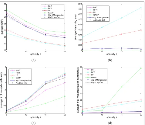
For the second configuration, the average values of the four metrics as a function of sparsity s are depicted in Fig. 3 for the BIHT, RFPI, LP, GAMP, and Algorithm 3 with fixedm = 1000 andn = 1000. Figure 3a, b depicts
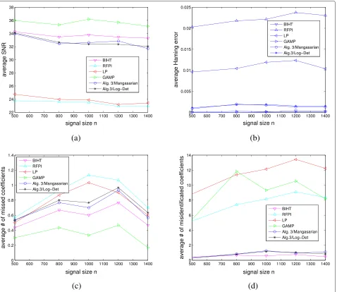
that BIHT, GAMP, and Algorithm 3 outperform the RFPI and LP in terms of values of SNR and the Hamming error. Figure 3c indicates that GAMP performs much bet-ter than the other algorithms in bet-terms of the number of missing nonzero coefficients while Fig. 3d indicates that GAMP performs much worse than the other algorithms in terms of the number of misidentified nonzero coefficients. For the third configuration, the average values of the four metrics as a function of signal sizesare depicted in Fig. 4 for the BIHT, RFPI, LP, GAMP, and Algorithm 3 with fixedm = 1000 ands = 10. The plots in Fig. 4a–c indicate that the GAMP performs best, the BIHT and Algorithm 3 perform similarly and exhibit much better performance than the LP and RFPI in terms of values of SNR, the Hamming error, and the number of miss-ing nonzero coefficients. Figure 4d shows that the BIHT and Algorithm 3 outperform the other algorithms for all tested values ofnin terms of the number of misidentified nonzero coefficients.
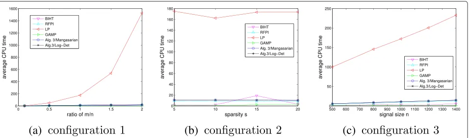
Finally, we compare the speed of the algorithms by measuring the average CPU time it takes each algorithm to produce the results showed in Figs. 2, 3, and 4. The experiments are performed under Windows 7 and Mat-lab 7.11 (R2010b) running on a laptop equipped with an Intel Core i5-2520M CPU at 2.50GHz and 4G RAM memory. When we implemented the BIHT, the num-ber of iterations is set to 1500. The MATLAB command
linprogwas adopted in the implementation of LP. The
source code of the GAMP was downloaded from the website of the first author of [10]. The source code of the RFPI was provided by the authors of [8]. The RFPI has two loops. The suggested number of outer-loop iter-ations is 20 while the number of inner-loop iteriter-ations is 200. The results of the experiments are depicted in Fig. 5. We find that both BIHT and GAMP are faster than the RFPI and Algorithm 3. The CPU time con-sumed by LP increases significantly, in particularly, when the size of the signal or the number of measurement increases.
(a)
(b)
(c)
7 Conclusions
In this paper, we proposed a new model and algorithm for 1-bit compressive sensing. The convergence analysis of the proposed algorithm was given. We demonstrated the performance of the algorithm for reconstruction from 1-bit measurements. In the future, it would be of interest to study the convergence of Algorithm 3 with the Man-gasarian function. This result would be highly needed to adaptively update all the parameters in Algorithm 3 so that consistent reconstruction can be achieved with improved accuracy.
Competing interests
The authors declare that they have no competing interests.
Acknowledgements
The authors would like to thank Ms. Na Zhang for her valuable comments and insightful suggestions which have brought improvements to several aspects of this manuscript. The authors would also like to thank Dr. Movahed for providing us his MATLAB source codes for the algorithm RFPI in [8]. The views and conclusions contained herein are those of the authors and should not be interpreted as necessarily representing the official policies or endorsement, either expressed or implied, of the Air Force Research Laboratory or the US Government.
This research is supported in part by an award from National Research Council via the Air Force Office of Scientific Research and by the US National Science Foundation under grant DMS-1522332.
Received: 7 July 2015 Accepted: 2 June 2016
References
1. E Candes, J Romberg, T Tao, Stable signal recovery from incomplete and inaccurate measurements. Commun. Pure Appl. Math.59(8), 1207–1223 (2006)
2. E Candes, T Tao, Near optimal signal recovery from random projections: universal encoding strategies?. IEEE Trans. Inf. Theory.52(12), 5406–5425 (2006)
3. PT Boufounos, RG Baraniuk, inProceedings of Conference on Information Science and Systems (CISS). 1-bit compressive sensing (IEEE, NJ, 2008), pp. 16–21
4. L Jacques, JN Laska, PT Boufounos, RG Baraniuk, Robust 1-bit compressive sensing via binary stable embeddings of sparse vectors. IEEE Trans. Inf. Theory.59, 2082–2102 (2013)
5. J Laska, Z Wen, W Yin, R Baraniuk, Trust, but verify: fast and accurate signal recovery from 1-bitcompressive measurements. IEEE Trans. Signal Process.59, 5289–5301 (2011)
6. Y Plan, R Vershynin, One-bit compressed sensing by linear programming. Commun. Pure Appl. Math.66, 1275–1297 (2013)
7. M Yan, Y Yang, S Osher, Robust 1-bit compressive sensing using adaptive outlier pursuit. IEEE Trans. Signal Process.60, 3868–3875 (2012) 8. A Movahed, A Panahi, G Durisi, A robust RFPI-based 1-bit compressive
sensing reconstruction algorithm. Information Theory Workshop (ITW), 2012 IEEE, Lausanne, 567–571 (2012). doi:10.1109/ITW.2012.6404739 9. A Movahed, A Panahi, Reed MC, inIEEE International Conference On
Acoustics, Speech, and Signal processing. Recovering signals with variable sparsity levels from the noisy 1-bit compressive measurements. (IEEE, 2014), pp. 6504–6508
10. U Kamilov, A Bourquard, A Amini, M Unser, One-bit measurements with adaptive thresholds. IEEE Signal Process. Lett.19(10), 607–610 (2012) 11. J-J Moreau, Proximité et dualité dans un espace hilbertien. Bull. Soc. Math.
France.93, 273–299 (1965)
12. ET Hale, W Yin, Y Zhang, Fixed-point continuation for1minimization:
methodology and convergence. SIAM J. Optimization.19, 1107–1130 (2008)
13. T Blumensath, ME Davies, Iterative hard thresholding for compressed sensing. Appl. Comput. Harmonic Anal.27, 265–274 (2009)
14. OL Mangasarian, Minimum-support solutions of polyhedral concave programs. Optimization.45, 149–162 (1999)
15. M Fazel, H Hindi, S Boyd, Log-det heuristic for matrix rank minimization with applications to Hankel and Euclidean distance matrices, American Control Conference. Proceedings of the 2003.3, 2156–2162 (2003). doi:10.1109/ACC.2003.1243393
16. R Chartrand, Exact reconstruction of sparse signals via nonconvex minimization. Signal Process. Lett. IEEE.14(10), 707–710 (2007) 17. R Chartrand, V Staneva, Restricted isometry properties and nonconvex
compressive sensing. Inverse Problems.24(3), 035020 (2008)
18. L Chen, Y Gu, The convergence guarantees of a non-convex approach for sparse recovery. IEEE Trans. Signal Process.62(15), 3754–3767 (2014) 19. M Hyder, K Mahata, An improved smoothed0approximation algorithm
for sparse representation. IEEE Trans. Signal Process.58(4), 2194–2205 (2010)
20. H Mohimani, M Babaie-Zadeh, C Jutten, A fast approach for overcomplete sparse decomposition based on smoothed norm. Signal Process. IEEE Trans.57(1), 289–301 (2009)
21. R Saaba, O Yilmaz, Sparse recovery by non-convex optimization instance optimality. Appl. Comput. Harmonic Anal.29(1), 30–48 (2010) 22. S Jokar, ME Pfetsch, Exact and approximate sparse solutions of
underdetermined linear equations. SIAM J. Sci. Comput.31(1), 23–44 (2008)
23. Y-B Zhao, D Li, Reweighted1-minimization for sparse solutions to
underdetermined linear system. SIAM J. Optim.22(3), 1065–1088 (2012) 24. A Chambolle, T Pock, A first-order primal-dual algorithm for convex
problems with applications to imaging. J. Math. Imaging Vision.40, 120–145 (2011)
25. Q Li, CA Micchelli, L Shen, Y Xu, A proximity algorithm accelerated by Gauss-Seidel iterations forL1/TVdenoising models. Inverse Problems.
28, 095003 (2012)
26. X Zhang, M Burger, S Osher, A unified primal-dual algorithm framework based on Bregman iteration. J. Sci. Comput.46, 20–46s (2011) 27. J-J Moreau, Fonctions convexes duales et points proximaux dans un
espace hilbertien. C. R. Acad. Sci. Paris Sér. A Math.255, 1897–2899 (1962) 28. HL Bauschke, PL Combettes,Convex Analysis and Monotone Operator
Theory in Hilbert Spaces, AMS Books in Mathematics. (Springer, New York, 2011)
29. L Shen, BW Suter, Bounds for eigenvalues of arrowhead matrices and their applications to hub matrices and wireless communications. EURASIP J. Adv. Signal Process. doi:10.1155/2009/379402
30. KR Davidson, SJ Szarek, inHandbook of the Geometry of Babach Spaces. Local operator theory, random matrices and Banach spaces, vol. 1 (Elsevier Science, Amsterdam: North-Holland, 2001), pp. 317–366
Submit your manuscript to a
journal and benefi t from:
7Convenient online submission 7Rigorous peer review
7Immediate publication on acceptance 7Open access: articles freely available online 7High visibility within the fi eld
7Retaining the copyright to your article