GENE EXPRESSION DATA ANALYSIS USING DATA
MINING ALGORITHMS FOR COLON CANCER
Archana Mishra
1, Rachna Devi
2, Sachin Shrivastava
3 1M.Tech Student,
2,3Assistant Professor, Department of Computer Science & Engineering,
SCET, Palwal (India)
ABSTRACT
The concept of Data mining is used in various medical applications like tumor classification, protein structure
prediction, gene classification, cancer classification based on microarray data, clustering of gene
expression data, statistical model of protein-protein interaction etc. Adverse drug events in prediction of
medical test effectiveness can be done based on genomics and proteomics through data mining
approaches. Cancer detection is one of the hot research topics in the bioinformatics. Data mining
techniques, such as pattern recognition, classification and clustering is applied over gene expression data
for detection of cancer occurrence and survivability. Classification of colon cancer dataset using weka library,
in which Logistics , Ibk, Kstar, NNge, ADTree , Random Forest Algorithms etc had shown 100 % correctly
classified instances, followed
by Navie Bayes classification and PART with 97.20 % accuracy. Kappa Statistic for Logis t ics , Ibk, Ks tar,
NNge, ADTree, Random Forest has shown Maximum. Mean absolute error and Root mean squared error are
shown low for Logistics , Ks tar and NNge. Using various Classification algorithms the cancer dataset can be
easily analyzed in order to obtain the better results.
Keywords: Data Mining, Colon Cancer, Dataset, ROC.
I. INTRODUCTION
In general, Data Mining refers to collecting or mining or extracting knowledge from large amounts of data
used in finding new interesting patterns and relationship related to the extracted data, discovering meaningful
new correlations, patterns, and trends by digging into large amounts of data stored in the warehouses. It
requires intelligent technologies and the compliance to explore the possibility of hidden knowledge that exists
in the data. Data mining algorithms and machine learning have exponential complexity and sometimes
require parallel computation [1,2].
It is observed that rapid developments in the field of Genomics and Proteomics have created huge biological data
to be analyzed. Making sense of the large biological data or analyzing the data by inferring structure or
generalization from the data has a great potential to increase the interaction between data mining and
bioinformatics. Bioinformatics and data mining provide exciting challenging research and application in the
areas of computational sciences [3].
The Waikato Environment for Knowledge Analysis (WEKA) provide a comprehensive collection of
machine learning algorithms and data pre-processing tools to researchers and practitioners on new
data sets [8, 9, 10]. Orange is an open source component based data mining and machine learning software suite
power for fast programming of new algorithms and developing complex data analysis procedures [4]
Cancer is a class of diseases characterized by out-of-control cell growth. It originates from small,
noncancerous (benign) tumors called denomatous polyps that form on the inner walls of the large intestine.
Colon cancer cells will invade and damage healthy tissue that is near the tumor causing many
complications. These cancer cells can grow in several places, invading and destroying other healthy tissues
throughout the body. This process itself is called metastasis, and the result is a more serious condition that
is very difficult to treat. Rectal cancer originates in the rectum, which is the last several inches of the large
intestine, closest to the anus. Colon cancer each year and it is the third most common cancer caused. Risk
factors Include a diet low in fiber and high in fat, certain types of colonic polyps, inflammatory bowel
disease (such as Crohn's disease or ulcerative colitis), and certain hereditary disorders [5][6]
The classification is done in order to fulfill various purposes like Predicting of tumor cells into benign or
malignant, classifying the secondary structure of proteins into alpha-helixes , beta-sheets or random
coils , Categorizing news stories as finance, weather, entertainment, sports , etc [7].
Association rule mining solves the problem of how to search efficiently for those dependencies . Single &
Multidimensional Association Rules are used to solve the problem. The prediction system has two stages :
feature selection and pattern classification stage. The feature selection can be considered as the gene selection,
which is to get the list of genes that might be informative for the prediction of tumor suppressor genes (`TSGs)
and proto ontogenesis by statistical, information theoretical methods. A classifier makes decision to which
category the gene pattern belongs at prediction stage [8][9].
II. MATHEMATICAL MODEL
2.1 System Requirements for the Present Work
Processor : Intel® Core ™ i3 CPU M 370 @ 2. 40 GHz 2. 40 GHz, Installed memory (RAM) : 4. 00 GB ( 3.
80 usable), Mother Board : HP Base Board, Hard Disk : 500 GB, OS : Windows 7 Professional (x64) (build
7600) and software such as WEKA and Orange.
2.2 Classification Algorithms
2.2.1 Bayesian Network
Bayesian networks are graphical representation for probabilistic relationships among a set of random variables.
A Bayesian network is an annotated directed acyclic graph (DAG) G that encodes a joint probability
distribution[10].
Algorithm
Step1: Given a finite set X= (X1 ,. ..,Xn ) of discrete random variables where each variable Xi may take values
from a finite set, denoted by Val(Xi ).
Step2: The nodes of the graph correspond to the random variables X1 ,..Xn . The links of the graph correspond to
the direct influence from one variable to the other. If there is a directed link from variable Xi to variable Xj .
Variable Xi will be a parent of variable Xj
Step3: Each node is annotated with a conditional probability distribution (CPD) that represents
where, denotes the parents of Xi inG. The pair (G,CPD) encodes the joint distribution p(X1 ,…,Xn ). A
unique joint probability distribution over X from G is factorized as: .
Naïve Bayesian classifier (Langley, 1995) is based on Bayes conditional probability rule is used for
performing classification tasks , assuming attributes as statistically independent. All attributes of the dataset
are considered independent and strong of each other.[11]
Algorithm
Step1: probability for each class is calculated in the dataset using P(C=Cj).
Step2: For each value xi of each attribute ai, probability is calculated using P(Xi|C=Cj)
Step3: Classify a new sample to class cj that have maximum probability P (C = Cj/X 1……Xn) using
Naïve-Bayes Classifier given below here denominator does not depend upon the value of Cj as:
2.2.3 Random Forest
Leo Breiman and Adele Cutler, 2001 developed Random forest algorithm, is an ensemble classifier that consists
of many decision tree and outputs the class that is the mode of the class's output by individual trees . Random
Forests grows many classification trees without pruning.[12]
Algorithm
Step1: Let N‟ be the number of training cases, and let „M ‟ be the number of variables in the classifier. Choose
m as input variables, to be used to determine the decision at a node of the tree; m should be much less than M.
Step2: Recourse training set for this tree by choosing N times with replacement from all N available training
cases (take a bootstrap sample). Rest of the cases to be estimated as error of the tree by predicting their classes.
Step3: For each node in the tree, randomly choose m variables, which should be based on the decision at that
node.
Step4: Calculate the best split based on these m variables in the training set. The value of m remains to be
constant during forest growing. Random forest is sensitive to the value of m.
Step5: Each tree is grown to the largest extent possible, into many classification trees without pruning, in
constructing a normal tree classifier.
III. METHODOLOGY
We will take following steps for our Methodology
Step1. We will take a dataset of Gene based Disease (we have taken colon cancer dataset) where the
Dataset has two classes i.e Positive and Negative.
Step2. Normalization process is required to be applied using Min-Max algorithm, in order to get the
Dataset values in a specific range.
Step3. PCA algorithm, we will apply the knowledge discovery processes and perform feature extraction in
order to identify the most relevant variables and determine the complexity and/or the general nature of
Disease patterns.
Step4. We will get a reduced dataset so as to perform further operations on it. Through the reduced dataset,
classifiers are to be found out which will help in training the machines through some technique.
Step5. We have used J48 And Navie Bayes Classification Algorithm for machine learning. Once the
machine learning is done, different association of genes are classified into different classes.
Step6. Testing is to be performed by giving sample inputs to the machine, which will in return give the
person is suffering from particular disease and if result is Negative then the person is not having colon
cancer.
Step7. On the basis of the various parameters after comparisons among the results.
IV. RESULTS AND DISCUSSIONS
4.1 Results for Classification Using J48
Colon Cancer attribute has been chosen randomly for colon-cancer-kent-ridge data set. J48 is applied on the data
set and the confusion matrix is generated for class gender having two possible values i.e. YES or NO.
Confusion Matrix:
a b classified as
33 72 | a = YES
25 170 | b = NO
For above confusion matrix, true positives for class a=YES is 33 while false positives is 72 whereas, for class
b=NO, true positives is 170 and false positives is 25 i.e. diagonal elements of matrix 33+170 =203 represents the
correct instances classified and other elements 25+72 = 97 represents the incorrect instances.
True positive rate = diagonal element/ sum of relevant row
False positive rate = non-diagonal element/ sum of relevant row
Hence,
TP rate for class a = 33/(33+72) = 0.314
FP rate for class a = 25/(25+170) = 0.128
TP rate for class b = 170/(25+170) = 0.871
FP rate for class b = 72/(33+72) = 0.685
Average TP rate = 0.677
Average FP rate = 0.491
Precision = diagonal element/sum of relevant column
Precision for class a = 33/(33+25) = 0.568
Precision for class b = 170/(170+72) = 0.702
F-measures = 2*precision*recall/(precision + recall)
F-measure for class a = 2*0.568*0.314/(0.568+0.314) = 0.404
F-measure for class b= 2*0.702*0.871/(0.702+0.871) = 0.778
4.2 Results for Classification Using Naïve Bayes Multinomial
Here same, Colon Cancer attribute has been chosen randomly for colon-cancer-kent-ridge data set. Naive Bayes
is applied on the data set and the confusion matrix is generated for class gender having two possible values i.e.
YES or NO.
Confusion Matrix:
a b ˛Al’ classified as
19 3 | a = YES
For above confusion matrix, true positives for class a=YES is 19 while false positives is 3 whereas, for class
b=NO, true positives is 5 and false positives is 35 i.e. diagonal elements of matrix 5 + 35 =40 represents the
correct instances classified and other elements 8+17 = 25 represents the incorrect instances.
TP rate for class a = 19/(19+3) =0.864
FP rate for class a = 5/(5+35) = 0.125
TP rate for class b = 35/(35+5) = 0.875
FP rate for class b = 3/(19+3) = 0.136
Average TP rate = 0.871
Average FP rate = 0.132
Precision = diagonal element/sum of relevant column
Precision for class a = 19/(19+5) = 0.792
Precision for class b = 35/(35+5) = 0.921
F-measures = 2*precision*recall/(precision + recall)
F-measure for class a = 2*0.792*0.864/(0.792+0.864) = 0.826
F-measure for class b = 2*0.921*0.875/(0.921*0.875) = 0.897
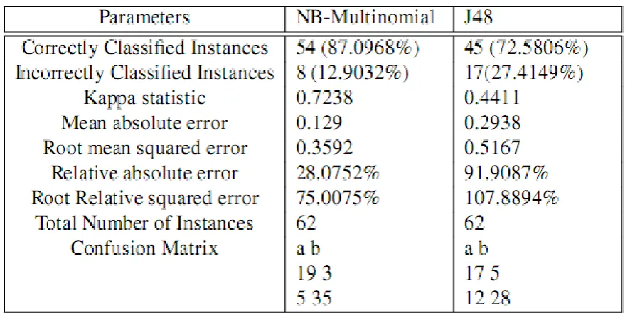
4.3 Comparative Result Analysis
Table 4.1: Table to Show Comparision Between Classification Algorithms
IV. CONCLUSION
From above experimental work we can conclude that correct instances generated by J48 and
NaïveBayesMultinomial, as well as performance evolution proves that the, NaïveBayesMultinomial is a simple
classifier technique to make a decision tree. Efficient result has been taken from bank dataset using weka tool in
the experiment. J48 classifier also shows good results. The experiment results shown in the study are about
classification accuracy and cost analysis. NaïveBayesMultinomial gives more classification accuracy for class
for both the classifier, with gender attribute, we can prove that NaïveBayesMultinomial is cost efficient than the
J48 classifier.
REFERENCES
[1] Mohammed J. Zaki, Shinichi Morishita, Isidore Rigoutsos, “Report on BIOKDD04: Workshop on Data
Mining in Bioinformatics”, in SIGKDD Explorations, vol. 6, no. 2, pp .153-154, 2004.
[2] J. Li, L. Wong, Q. Yang, “Data Mining in Bioinformatics”, IEEE Intelligent System, IEEE Computer
Society . Indian Journal of Computer Science and Engineering, vol 1 no 2, pp . 114-118, 2005.
[3] R. P. Kumar, M . Rao, D. Kaladhar, “Data Categorization and Noise Analysis in Mobile Communication
Using Machine Learning Algorithms”, Wireless Sensor Network, vol. 4, no.4, pp . 113-116, 2012.
[4] Mark H. E. Frank, Geoffrey Holmes, Bernhard Pfahringer, Peter Reutemann, Ian H. Witten, “The WEKA
data mining software: an update“ , SIGKDD Explorations, vol. 11, no.1, pp .10-18, 2009.
[5] D. J. Hand, “Statistics and data mining: intersecting disciplines“ , SIGKDD Explorations, vol. 1, no. 1,
pp . 16-19, 1999.
[6] C Apte, E Grossman, E Pednault , B Rosen, F Tipu, B White, "Insurance risk modeling using data mining
technology", Proceedings of PADD99: The Practical Application of Knowledge Discovery and Data
Mining, pp .39-47, 1999.
[7] Liu, Bing, Chee Wee Chin, Hwee Tou Ng. "Mining topic-specific concepts and definitions on the
web." Proceedings of the 12th international conference on World Wide Web. ACM , pp .251-260, 2003.
[8] M .K. Jakubowski, Q. Guo, M. Kelly , “Tradeoffs between lidar pulse density and forest measurement
accuracy ”, Remote Sensing of Environment , vol. 130, pp . 245-253, 2013.
[9] E. Frank, M . Hall, L. Trigg, G. Holmes, I. H. Witten, “Data mining in bioinformatics using Weka ”,
Bioinformatics, vol. 20, no. 15, pp . 2479-2481, 2004.
[10] M . Hall, E. Frank, G. Holmes, B. Pfahringer, P. Reutemann, I.H. Witten, “The WEKA data mining
software: an update ACM SIGKDD Explorations Newsletter, vol. 11, no. 1, pp .10-18, 2009.
[11] Tomaž Curk, Janez Demšar, Qikai Xu, Gregor Leban, Uroš Petrovič, Ivan Bratko, Gad Shaulsky ,
Blaž Zupan, “Microarray data mining with visual programming”, Bioinformatics, vol. 21, no. 3, pp .
396-398, 2005.
[12] R. W. Burt , J. S. Barthel, K. B. Dunn, D. S. David, E. Drelichman, J. M . Ford, et al, “Colorectal cancer
screening”, Journal of the National Comprehensive Cancer Network, vol. 8, no. 1, pp . 8-61, 2010.
[13] David Cunningham, Wendy Atkin, Heinz -Josef Lenz , Henry T Lynch, Bruce Minsky , Bernard
Nordlinger, Naureen Starling, “Colorectal cancer ”, The Lancet , vol. 375, no. 9719, pp . 1030-1047, 2010.
[14] R. A. Smith, V. Cokkinides, D. Brooks, D. Saslow, O. W. Brawley , “Cancer screening in the United
States, 2010: a review of current American Cancer Society guidelines and issues in cancer screening”,
CA: a cancer journal for clinicians, vol. 60, no.2, pp . 99-119, 2010.
[15] K. Mehmed, "Data Mining: Concepts, Models, Methods And Algorithms." IEEE Computer Society, IEEE
Press, 2003.
[16] W. J. Frawley , G. Piatetsky -Shapiro, C. J. Matheus, “Knowledge discovery in databases: An
overview”, AI magazine, vol. 13, no. 3, pp . 57, 1992.
[17] H. Lieberman, D. Maulsby , “Instructible agents: Software that just keeps getting better”, IBM Systems
[18] R. Rada, “Expert systems and evolutionary computing for financial investing: A review”, Expert
systems with applications, vol. 34, no. 4, pp . 2232-2240, 2008.
[19] Cho Sung-Bae, Hong-Hee Won, "Machine learning in DNA microarray analysis for cancer classification",
In Proceedings of the First Asia-Pacific bioinformatics conference on Bioinformatics, vol. 19, pp .