Volume 3, No. 7, Nov-Dec 2012
International Journal of Advanced Research in Computer Science
RESEARCH PAPER
Available Online at www.ijarcs.info
ISSN No. 0976-5697
Independence of Redundant Attributes in the Attribute Reduction Algorithm
Nguyen Duc Thuan
Information Systems Departement Nha Trang University Nha Trang City,
Khanh Hoa Province, Vietnam [email protected]
Abstract: We proposed an attribute reduction algorithm of decision system. It based on a family covering rough set. In this Algorithm, the independence of redundant attributes is critical to the correctness and complexity of the algorithm. This paper presents removing a redundant attribute does not affect the property of a nonredundant attribute.
Keywords: redundant attribute, attribute reduction, decision system, covering rough sets, consistent decision system.
I. INTRODUCTION
Attribute reduction of an information system is a key problem in rough set theory and its application. It has been proven that finding the minimal reduct of an information system. In [2], Cheng Degang et al. have defined consistent and inconsistent covering decision system and their attribute reduction. They gave an algorithm to compute all the reducts of decision systems. Their method based on discernibility matrix. But, in rough set theory, it has been proved that finding all the reduct of information systems (decision tables) is NP-complete. Hence, sometime we only need to find an attribute reduction. Using some results of Chen Degang et al, we proposed an algorithm which is finding a minimal attribute reduct information decision system [1]. Removing a redundant attributes can affect the property of the remaining properties (e.g. nonredundant attribute X can become redundant attribute, after a redundant attribute Z removed because there are the relationships between the attributes). This paper show the independence of redundant attributes in attribute reduction algorithm based on family covering rough sets.
The remainder of this paper is structured as follows. In section 2 briefly introduces some relevant concepts and results. Section 3, we present our attribute reduction algorithm based on family covering rough sets. Section 4 presents two propositions about the independence of redundant attributes.
II. SOMERELEVANTCONCEPTSAND
RESULTS
In this section, we first recall the concept of a cover and then review the existing research on covering rough sets of Cheng Degang et al. [2]
A. Covering rough sets and induced covers:
Definition 2.1 Let U be a universe of discourse, C a family of subsets of U. C is called a cover of U if no subset in C is empty and ∪C = U.
Definition 2.2 Let C = {C1, C2..., Cn} be a cover of U. For every x∈U, let Cx = ∩{Cj: Cj∈C, x∈Cj}. Cov(C) = {Cx: x∈U} is then also a cover of U. We call it induced over of C.
Definition 2.3 Let ∆= {Ci: i=1, m} be a family of covers of U. For every x∈U, let ∆x= ∩{Cix: Cix∈ Cov (Ci), x∈Cix} then Cov (∆) = {∆x: x∈U} is also a cover of U. We call it the induced cover of ∆.
Clearly ∆x is the intersection of all the elements in every Ci including x, so for every x∈U, ∆x is the minimal set in Cov(∆) including x. If every cover in ∆ is an attribute, then
∆x= ∩{Cix: Cix∈Cov(Ci), x∈Cix} means the relation among Cix is a conjunction. Cov(∆) can be viewed as the intersection of covers in ∆. If every cover in ∆ is a partition, then Cov(∆) is also a partition and ∆x is the equivalence class including x. For every x, y ∈ U, if y ∈∆x, then ∆x⊇
∆y, so if y ∈∆x and x ∈∆y, then ∆x=∆y. Every element in Cov(∆) can not be written as the union of other elements in Cov(∆). We employ an example to illustrate the practical meaning of Cx and ∆x.
For every X ⊆ U, the lower and upper approximation of X with respect to Cov(∆) are defined as follows:
( )X { x: x X},
∆ = ∪ ∆ ∆ ⊆
( )∆ X = ∪ ∆ ∆ ∩{ x: x X ≠ ∅}
The positive, negative and boundary regions of X relative to ∆ are computed using the following formulas respectively:
( ) ( ), ( ( ), ( ) ( ) ( )
POS X X NEG U X
BN X X X
∆ ∆
∆
= ∆ − ∆
= ∆ − ∆
Clearly in Cov(∆), ∆x is the minimal description of object x.
B. Attribute reduction of consistent and inconsistent decision systems:
Definition 2.4 Let ∆ = {Ci: i=1,..m} be a family of covers of U, D is a decision attribute, U/D is a decision partition on U. If for ∀x∈U, ∃Dj∈U/D such that ∆x ⊆ Dj, then decision system (U,∆,D) is called a consistent covering decision system, and denoted as Cov(∆)≤ U/D. Otherwise, (U,∆,D) is called an inconsistent covering decision system. The positive region of D relative to ∆ is defined as
/ ( ) ( )
X U D
POS∆ D X
∈
Remark 2.1 Let D={d}, then d(x) is a decision function d: U → Vd of the universe U into value set Vd. For every xi, xj∈U , if ∆xi ⊆∆xj, then d(xi) = d([xi]D) = d(∆xi) = d(∆xj) = d(xj) = d([xj]D). If d(∆xi) ≠ d(∆xj), then ∆xi
∩∆xj = ∅, i.e ∆xi⊄∆xj and ∆xj⊄∆xi.
Definition 2.5 Let (U,∆, D= {d}) be a consistent covering decision system. For Ci ∈∆ , if Cov(∆-{Ci}) ≤ U/D, then Ci is called superfluous relative to D in ∆ , otherwise Ci is called indispensable relative to D in ∆. For every P ⊆∆ satisfying Cov(P) ≤U/D , if every element in P is indispensable, i.e., for every Ci∈P, Cov(∆-{Ci}) ≤ U/D is not true, then P is called a reduct of D relative to D, relative reduct in short. The collection of all the indispensable elements in D is called the core of ∆ relative to D, denoted as CoreD(∆). The relative reduct of a consistent covering decision system is the minimal set of conditional covers (attributes) to ensure every decision rule still consistent. For a single cover Ci, we present some equivalence conditions to judge whether it is indispensable.
Definition 2.6 Suppose U is a finite universe and ∆ = {Ci: i=1,..m} be a family of covers of U, Ci∈∆, D is a decision attribute relative ∆ on U and d: U → Vd is the decision function Vd defined as d(x) = [x]D. (U,∆,D) is an inconsistent covering decision system, i.e., POS∆(D)≠U. If POS∆(D)=POS∆-{Ci}(D), then Ci is superfluous relative to D in ∆. Otherwise Ci is indispensable relative to D in ∆. For every P⊆∆, if every element in P is indispensable relative to D, and POS∆(D)=POSP(D), then P is a reduct of POS∆(D)=POS∆-{Ci}(D) relative to D, called relative reduct in short. The collection of all the indispensable elements relative to D in ∆ is the core of ∆ relative to D, denoted by CoreD(∆).
C. Some results of Chang et al:
Theorem 2.1 ([2]) Supposing U is a finite universe and
∆ = {Ci: i=1,..m} be a family of covers of U, the following statements hold:
a. ∆x = ∆y if and only if for every Ci∈∆ we have Cix = Ciy.
b. ∆x⊃∆y if and only if for every Ci∈∆ we have Cix⊇ Ciy and there is a Ci∈∆ such that Ci0 x⊃ Ci0 y .
c. ∆x⊄∆y and ∆y⊄∆x hold if and only if there are Ci, Cj
∈∆ such that Cix ⊂ Ciy and Cjx⊃ Cjy or there is a Ci0
∈∆ such that Ci0 x⊄ Ci0 y and Ci0 y⊄ Ci0 x .
Theorem 2.2 ([2]) Suppose Cov(∆)≤ U/D, Ci∈∆, Ci is then indispensable, i.e., Cov(∆-{Ci}) ≤ U/D is not true if and only if there is at least a pair of xi, xj∈U satisfying d(Dxi)≠ d(Dxj), of which the original relation with respect to ∆ changes after Ci is deleted from ∆.
Theorem 2.3 ([2]) Suppose Cov(∆) ≤ U/D,P ⊆∆ , then Cov(P) ≤ U/D if and only if for xi, xj∈U satisfying d(∆xi) ≠ d(∆xj), the relation between xi and xj with respect to ∆ is equivalent to their relation with respect to P, i.e., ∆xi ⊄∆xj and ∆xj⊄∆xi⇔ Pxi⊄ Pxj, Pxj⊄ Pxi.
Theorem 2.4 ([2]) Inconsistent covering decision system (U,∆,D = {d}) have the following properties:
a. For ∀xi∈U, if ∆xi ⊂ POS∆(D), then ∆xi ⊆[xi ]D; if
∆xi ⊄ POS∆(D), then for ∀xk∈U, ∆xi ⊆[xk]D is not true.
b. For any P⊆∆, POSP(D)= POS∆(D) if and only if
( ) ( )
P X = ∆ X for ∀X∈U/D.
c. For any P⊆∆, POSP(D)= POS∆(D) if and only if
∀xi∈U, ∆xi ⊆[xi]D⇔ Pxi ⊆[xi]D.
III. ALGORITHMOFATTRIBUTEREDUCTION
In this section, we propose a new algorithm of attribute reduction. Propositions 3.1 and 3.2 are theoretic foundation for our proposing. This algorithm finds an approximately minimal reduct.
A. Two propositions as a base for new algorithm:
Proposition 3.1 Let (U,∆,D={d}) be a covering decision system. P ⊆∆, then we have:
a. (U,∆,D={d}) is a consistent covering decision system when it holds:
[ ]
x D
x U x
x U
∈
∆ ∩ = ∆
∑
b. Suppose Cov(∆)≤ U/D, Ci ∈∆, Ci is then indispensable, i.e., Cov(∆-{Ci}) ≤ U/D is true if and only if
( xi xj ( xi xj) ( xi) ( xj) 0
xi U xj U
P P d d
∈ ∈
∆ ∩ ∆ ∪ ∩ ∆ − ∆ =
∑ ∑
Where Cov(∆-{Ci})={Px : x∈U}, Cov(∆)= {∆x : x ∈U} Proof:
a) By define of a consistent covering decision system, clearly for every x∈U, ∆x ⊆ [x]D is always true, thus we have
[ ]
x xD x
∆ ∩ = ∆
i.e
[ ]
x D
x U x
x U
∈
∆ ∩ = ∆
∑
b) Let Cov(∆-{Ci})={Px : x∈U} = Cov(P), Cov(∆)= {∆x : x ∈U, by theorem 2.3, P is a reduct or Ci is indispensable, for xi, xj ∈U satisfying d(∆xi) ≠ d(∆xj), the relation between xi and xj with respect to ∆ is equivalent to their relation with respect to P, i.e., ∆xi⊄
∆xj and ∆xj⊄∆xi⇔ Pxi⊄ Pxj, Pxj⊄ Pxi. Follow remark 2.1, If d(∆xi) ≠ d(∆xj), then ∆xi∩∆xj = ∅, i.e
(∆ ∩ ∆ ∪xi xj) (Pxi∩Pxj) =0
If xi, xj∈U satisfying d(∆xi) = d(∆xj) then
( xi) ( xj) 0 d ∆ − ∆d =
In other words, it holds:
( xi xj ( xi xj) ( )xi ( )xj 0
xi U xj U
P P d d
∈ ∈
∆ ∩ ∆ ∪ ∩ ∆ − ∆ =
∑ ∑
This completes the proof.
Proposition 3.2 Let (U,∆,D={d}) be an inconsistent covering decision system. P ⊆ ∆, POSP(D) = POS ∆(D) if and only if ∀xi∈U,
[ ] [ ] 0
xi i D xi i D
xi U xi xi
x P x
P
∈
∆ ∩ ∩
− =
∆
∑
Proof:
By theorem 2.4, from third condition ∀xi∈U, ∆xi⊆[xi]D
⇔ Pxi⊆ [xi]D i.e ∀xi∈U, [ ]
xi xD xi
∆ ∩ = ∆ ⇔ Pxi∩
[ ]
x D = PxiB. Algorithm of attribute reduction in covering decision system:
Input: A covering decision system S= (U,∆,D={d})
Output: One product RD of ∆. Method
Step 1: Compute
[ ]
x D
x U x
x CI
∈
∆ ∩ =
∆
∑
Step 2: If CI = |U| {S is a consistent covering decision system} then goto Step 3 else goto Step 5.
Step 3: Compute
, ( ),
x d x x U
∆ ∆ ∀ ∈
Step 4: Begin For each Ci∈∆ do
if
( xi xj ( xi xj) ( xi) ( xj) 0
xi U xj U
P P d d
∈ ∈
∆ ∩ ∆ ∪ ∩ ∆ − ∆ =
∑ ∑
{Where ∆ - {Ci} = {Px : x∈U}} then ∆:= ∆ - {Ci};
Endfor; goto Step 6.
End; Step 5: Begin For each Ci∈∆ do
if
[ ] [ ] 0
xi i D xi i D
xi U xi xi
x P x
P
∈
∆ ∩ ∩
− =
∆
∑
then ∆:= ∆ - {Ci}; {Where ∆ - {Ci} = {Px : x∈U}} Endfor;
End;
Step 6: RD=∆; the algorithm terminates.
By using this algorithm, the time complexity to find one reduct is polynomial.
At the first step, the time complexity to compute CI is O(|U|).
At the step 2, the time complexity is O(1). At the step 3, the time complexity is O(|U|).
At the step 4, the time complexity to compute ∑∑() is O(|U|2), from i=1..|∆|, thus the time complexity of this step is O(|∆||U|2).
At the step 5, the time complexity is the same as step 4. It is O(|∆||U|2).
At the step 6, the time complexity is O(1).
Thus the time complexity of this algorithm is O(|∆||U|2) (Where we ignore the time complexity for computing ∆xi, Pxi, i= 1..|∆|).
IV. ILLUSTRATIVEEXAMPLES
A. Example for a consistent covering decision system: Suppose U = {x1, x2, .., x9}, ∆ = {Ci, i=1..4}, and C1={{x1, x2, x4, x5, x7, x8},{x2, x3, x5, x6, x8, x9}}, C2={{x1, x2, x3, x4, x5, x6},{x4, x5, x6, x7, x8, x9}}, C3={{x1, x2, x3},{x4, x5, x6, x7, x8, x9},{x8, x9}},
C4={{x1, x2, x4, x5},{x2, x3, x5, x6},{x7, x8},{x5, x6, x8, x9}}
U/D={{x1, x2, x3}, {x4, x5, x6}, {x7, x8, x9}}
where, ∆i=∆xi, Pi is Pxi (for short) Step 1:
∆1={x1, x2}, ∆2={x2}, ∆3={x2, x3}, we have d(∆1) = d(∆2) = d(∆3) = 1, because ∆1, ∆2, ∆3 ⊆ {x1, x2, x3},
∆4={x4, x5}, ∆5={x5}, ∆6={x5, x6}, we have d(∆4) = d(∆5) = d(∆6) = 2, because ∆4, ∆5, ∆6 ⊆ {x4, x5, x6},
∆7={x7, x8}, ∆8={x8}, ∆9={x8, x9}, we have d(∆7) = d(∆8) = d(∆9) = 3, because ∆7, ∆8, ∆9 ⊆ {x7,x8, x9}
CI = 9 ⇒ S is consistent system. Step 2:
P - {C1}:
P1={x1, x2}, P2={x2}, P3={x2, x3}, P4={x4,x5}, P5={x5}, P6={x5, x6}, P7={x7, x8}, P8={x8}, P9={x8, x9}
( xi xj ( xi xj) ( xi) ( xj) 0
xi U xj U
P P d d
∈ ∈
∆ ∩ ∆ ∪ ∩ ∆ − ∆ =
∑ ∑
∆=∆ - {C1} = {C2, C3, C4}. Step 3:
P=∆ - {C2}
P1={x1, x2}, P2={x2}, P3={x2, x3}, P4={x4, x5}, P5={x5}, P6={x5, x6}, P7={x7, x8}, P8={x8}, P9={x8, x9}
( xi xj ( xi xj) ( xi) ( xj) 0
xi U xj U
P P d d
∈ ∈
∆ ∩ ∆ ∪ ∩ ∆ − ∆ =
∑ ∑
∆=∆ - {C2} = {C3, C4} Step 4:
P= ∆ - {C3}:
P1={x1, x2, x4, x5}, P2={x2}, P3={x2, x3, x5, x6}, P4={x4, x5}, P5={x5}, P6={x5, x6},
P7={x4, x5, x7, x8}, P8={x5, x8}, P9={x5, x6, x8, x9}
( xi xj ( xi xj) ( xi) ( xj) 0
xi U xj U
P P d d
∈ ∈
∆ ∩ ∆ ∪ ∩ ∆ − ∆ ≠
∑ ∑
(we can see (∆1∩∆4)=∅, but (P1∩P4)≠∅, |d(∆1)-d(∆4)|≠0)
∆= {C3,C4}. Step 5:
P= ∆ - {C4}
P1={x1, x2, x3}, P2={x1, x2, x3}, P3={x1, x2, x3},
P4={x4, x5, x6, x7, x8, x9}, P5={x4, x5, x6, x7, x8, x9}, P6={x4,x5,x6,x7,x8,x9}
P7={x7, x8, x9}, P8={x7, x8, x9}, P9={x7, x8, x9}
( xi xj ( xi xj) ( xi) ( xj) 0
xi U xj U
P P d d
∈ ∈
∆ ∩ ∆ ∪ ∩ ∆ − ∆ ≠
∑ ∑
(we can see (∆6∩∆7) =∅, but (P6∩P7)≠∅, |d(∆6)-d(∆7)|≠0)
∆= {C3,C4}. Step 6:
RD= {C3,C4} is a reduct. i.e. attributes with respect to C1, C2 are deleted.
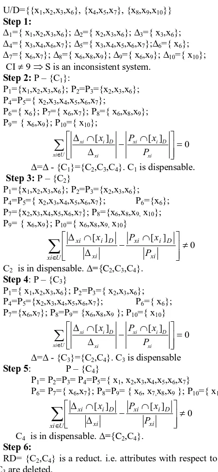
B. Example for a inconsistent covering decision system:
Suppose U={x1,x2,x3,x4,x5,x6,x7,x8,x9,x10} and {Ci, i=1..4} C1={{x1,x2,x3,x4,x6,x7,x8,x9,x10},{x3,x4,x6,x7},{x3,x4,x5,x6, x7}}
C2={{x1,x2,x3,x4,x5,x6,x7},{x6,x7,x8,x9},{x10}} C3={{x1,x2,x3,x6,x8,x9,x10},{x2,x3,x4,x5,x6,x7,x9}}
U/D={{x1,x2,x3,x6}, {x4,x5,x7}, {x8,x9,x10}} Step 1:
∆1={ x1,x2,x3,x6}; ∆2={ x2,x3,x6}; ∆3={ x3,x6};
∆4={ x3,x4,x6,x7}; ∆5={ x3,x4,x5,x6,x7};∆6={ x6};
∆7={ x6,x7}; ∆8={ x6,x8,x9}; ∆9={ x6,x9}; ∆10={ x10}; CI ≠ 9 ⇒ S is an inconsistent system.
Step 2: P – {C1}:
P1={x1,x2,x3,x6}; P2=P3={x2,x3,x6}; P4=P5={ x2,x3,x4,x5,x6,x7};
P6={ x6}; P7={ x6,x7}; P8={ x6,x8,x9}; P9= { x6,x9}; P10={ x10};
[ ] [ ] 0
xi i D xi i D
xi U xi xi
x P x
P ∈ ∆ ∩ ∩ − = ∆
∑
∆=∆ - {C1}={C2,C3,C4}. C1 is dispensable. Step 3: P – {C2}
P1={x1,x2,x3,x6}; P2=P3={x2,x3,x6}; P4=P5={ x2,x3,x4,x5,x6,x7}; P6={x6}; P7={x2,x3,x4,x5,x6,x7}; P8={x6,x8,x9, x10}; P9= { x6,x9}; P10={ x6,x8,x9, x10}
0 ] [ ] [ ≠ ∩ − ∆ ∩ ∆
∑
∈U xi xi D i xi xi D i xi P x P xC2 is in dispensable. ∆={C2,C3,C4}. Step 4: P – {C3}
P1={ x1,x2,x3,x6}; P2=P3={ x2,x3,x6}; P4=P5={x2,x3,x4,x5,x6,x7}; P6={ x6}; P7={x6,x7}; P8=P9= {x6,x8,x9 }; P10={ x10}
[ ] [ ] 0
xi i D xi i D
xi U xi xi
x P x
P ∈ ∆ ∩ ∩ − = ∆
∑
∆=∆ - {C3}={C2,C4}. C3 is dispensable Step 5: P – {C4}
P1= P2=P3= P4=P5={ x1, x2,x3,x4,x5,x6,x7}
P6= P7={ x6,x7}; P8=P9= { x6, x7,x8,x9 }; P10={ x10}
0 ] [ ] [ ≠ ∩ − ∆ ∩ ∆
∑
∈U xi xi D i xi xi D i xi P x P xC4 is in dispensable. ∆={C2,C4}. Step 6:
[image:4.595.40.265.49.536.2]RD= {C2,C4} is a reduct. i.e. attributes with respect to C1, C3 are deleted.
Table I. Comparision with results of Chen Degang et al
Algorithm of Chen Degang et al New Algorithm Example 1
Red(∆) = {{C3, C4}, {C2, C3}} RD= {C3,C4} Example 2
Red(∆) = {{C2, C4}, {C2, C3}} RD= {C2,C4}
Note: Where Red(∆) = Collection all reducts of ∆; RD is a reduct of ∆
V. INDEPENDENCEOFREDUNDANT
ATTRIBUTES
In this section, we show the independence of redundant attributes in the algorithms above. This property is presented through problem:
Is there a conversion of a nonredundant covering into a redundant covering when a redundant covering removed?
We have two propositions:
Proposition 4.1 Let T= (U,∆,D={d}) be a consistent covering decision system has
a. is a family covering ∆={C1, C2, .., Cn} b. Cov(∆)≤U/D
Consider 2 family covering P1, P2 statisfy: P2⊆P1⊆∆, Cov(Pi)≤U/D, i=1,2.
Then ∀Ck∈P2⊆P1, if Ck is nonredundant in P1 then Ck is nonredundant in P2 (*)
Proof:
We need to prove that if Ck is redundant in P2 then Ck is redundant in P1.
Let P11 = P1-{Ck}, P22 = P2-{Ck}.
Suppose Ck is nonredundant in P1 , then Cov(P1 -{Ck})≤U/D is not true.
Cov(P1-{Ck})≤U/D is not true ⇔∃xi0,xj0∈U such that d(P1xi0) ≠d(P1xj0), P1xi0∩P1xj0=∅ but P11xi0∩P11xj0≠∅
If Ck is redundant in P2⇔ Cov(P2-{Ck})≤U/D. ⇔
∀xi,xj ∈U, d(P2xi) ≠ d(P2xj), we get P2xi∩P2xj=∅ and P22xi∩P22xj=∅
Since P2⊆P1⊆∆, Cov(Pi)≤U/D, i=1,2, so
∀xi,xj ∈U, d(P1xi) ≠ d(P1xj) implies that
P1xi∩P1xj=∅ and P2xi∩P2xj=∅ Clearly, P2⊆P1 implies that ∀xi∈U, ∀Ck∈P2⊆P1 :P11xi
⊆ P22xi ,
Combining (1)(2)(3)(4) gives a contradiction: ∅≠ P11xi0∩P11xj0⊆P22xi0∩P22xj0=∅.
In other words, we have (*). The proof is complete. Proposition 4.2 Let T= (U,∆,D={d}) be an inconsistent covering decision system has
a. ∆ is a family covering ∆={C1, C2, .., Cn} b. POS∆(D)≠U
Consider 2 family covering P1, P2⊆∆ statisfy: a) P2⊆ P1
b) 1( ) 2( )
P P
POS D =POS D ≠U
Then ∀Ck∈P2⊆P1, if Ck is nonredundant in P1 then Ck is nonredundant in P2 (*)
Proof:
In the same way as in Proposition 4.1, we need to prove that if Ck redundant in P2 then Ck redundant in P1.
Let P11=P1-{Ck}, P22=P2-{Ck}. If Ck is redundant in P2 then
) ( )
( 2
22 D POS D
POSP = P
D i x D i x
i U P x P x
x
i
i [ ] [ ]
: 22 ⊆ ⇔ 2⊆
∈ ∀
⇔
Suppose Ck is nonredundant in P1 , we have :
11( ) 1( )
P P
POS D ≠POS D
D
x x
P U
x0 : 11 [ 0]
0 ⊄ ∈
∃
⇔ và
0 1
0
[ ]
x D
P ⊆ x
Since POSP1(D)=POSP2(D)≠U, it follows that
D x
D
x x P x
P1 [ 0] 2 [ 0]
0
0 ⊆ ⇔ ⊆
By (α)(β)(γ), we get
D x D x D x D
x x P x P x P x
P U
x : [ ] , [ ] , [ ] , [ 0]
11 0 22 0 2 0 1 0 0 0 0
0 ⊆ ⊆ ⊆ ⊄
∈ ∃
Since P 22⊆
P11, it follows that 220 11
x
xo P
P ⊆ which contradicts with
D x
D
x x P x
P11 [ 0] , 22 [ 0]
0
0 ⊄ ⊆
VI. CONCLUSION
Independence of redundant attributes in the Attribute reduction algorithm based on a family covering rough sets allows we process only one time to remove redundant attributes. This determines the performance of the algorithm above.
VII. REFERENCES
[1] Nguyen Duc Thuan, “A family of covering rough sets based algorithm for reduction attributes”, International journal of Computer Theory and Engineering, vol.2, No.2, pp.181–184, April 2010.
[2] Chen Degang, Wang Changzhong, Hu Quinghua, “A new approach to attribute reduction of consistent and
inconsistent covering rough sets”, Information Sciences, 177 (2007) 3500-3518
[3] Guo-Yin Wang, Jun Zhao, Jiu-Jiang An, Yu Wu, “Theoretical study on attribute reduction of rough set theory: Comparision of algebra and information views”, Proceedings of the Third IEEE International Conference on Cognitive Informatics (ICCI’04), 2004
[4] Ruizhi Wang, Duoqian Miao, Guirong Hu, “Descernibility Matrix Based Algorithm for Reduction of Attributes”, IAT Workshops 2006: 477- 480