R E S E A R C H
Open Access
Particle filter track-before-detect implementation
on GPU
Xu Tang
*, Jinzhou Su, Fangbin Zhao, Jian Zhou and Ping Wei
Abstract
Track-before-detect (TBD) based on the particle filter (PF) algorithm is known for its outstanding performance in detecting and tracking of weak targets. However, large amount of calculation leads to difficulty in real-time applications. To solve this problem, effective implementation of the PF-based TBD on the graphics processing units (GPU) is proposed in this article. By recasting the particles propagation process and weights calculating process on the parallel structure of GPU, the running time of this algorithm can greatly be reduced. Simulation results in the infrared scenario and the radar scenario are demonstrated to compare the implementation on two types of the GPU card with the CPU-only implementation.
Keywords:Track-before-detect, Particle filter, GPU
1. Introduction
Classical target detection and tracking is performed on the basis of pre-processed measurements, which are composed of the threshold output of the sensor. In this way, no effective integrations over time can be taken place and much information is lost. To avoid this problem, the track-before-detect (TBD) technique is developed to use directly the un-threshold or low threshold measurements of sensors to utilize the raw information. The TBD-based procedures jointly process more consecutive measurements, thus can increase the signal-to-noise ratio (SNR), and realize the detection and tracking of weak targets simultaneously.
The scenarios faced by TBD are almost nonlinear and non-Gaussian, so the particle filter (PF) [1] is a reason-able solution. The PF is a Monte Carlo simulation method and widely used in target tracking of linear or nonlinear dynamic systems [2,3]. Salmond and coauthors [4,5] first introduced the PF implementation of TBD (PFTBD) in infrared scenario. Then, Rutten et al. [6-8] proposed several improved PFTBD algorithms. Boers and Driessen [9] extended the work of PFTBD into the radar targets detection and the tracking application. PFTBD algorithms have demonstrated the improved track accuracy and the ability to follow the low SNR
targets but at the price of an extreme increase of the computational complexity.
In recent years, the field programmable gate array (FPGA) and the graphics processing unit (GPU) are the most important architectures in parallel computing. As the rapid development of GPU technology, GPU is fam-ous for its significant ability in parallel computing for both the graphic processing and the general-purpose computing. Moreover, the compute unified device archi-tecture (CUDA) [10] is introduced to facilitate a hybrid utilization of GPU and central process unit (CPU) [11]. FPGA has been used to implement PFs, such as in [12,13]. However, with the increasing of number of particles, GPU is expected to obtain a better perform-ance than FPGA. More specifically, the PF algorithms have been implemented on GPU [14-16], and achieve significant speedup ratio over the implementations on the traditional CPU fashion but with no losing the per-formance for its float point computation ability.
From the best of the authors’ knowledge, no PFTBD algorithm implemented on GPU is given in the litera-ture. In this article, we propose a novel implementation of PFTBD algorithm on GPU by the CUDA program-ming. Concerned with the difficulty of PFTBD beyond the PF, new scheme to dispatch the GPU resources for particles are developed and the programming about the likelihood ratio area are considered carefully.
* Correspondence:[email protected]
Department of Electronic Engineering, University of Electronic Science and Technology of China, Chengdu, People’s Republic of China
Simulations in both the infrared scenario and the radar scenario are given. Two types of the GPU card are utilized. The implementations of PFTBD algorithm on both of them achieve significant speedup over the CPU-only implementation. The initial version of this research first appeared in [17].
This article is organized as follows. Section 2 reviews the theory about PFTBD. In Section 3, we discuss the details about the parallel implementation of PFTBD on GPU and CUDA programming. The simulations results and discussions can be found in Section 4. Finally, we conclude this article in Section 5.
2. PFTBD theory
In this article, the single target recursive TBD algorithms are presented. The way to process raw measurement of sensor in TBD is different from the classical target tracking methods. The measurement model and the way of data processing vary with the sensor type. The models are set mathematically with a summary of the infrared scenario and the radar scenario. The simulations in Section 4 are based on these models.
2.1. Target model and measurement model of infrared sensor
Consider an infrared sensor that collects a sequence of two-dimensional images of the surveillance region, as in [7]. When the target presents, the state of the target is evolving as a constant velocity (CV) model. The time evolution model of the target used here is a linear Gaussian process
Xk¼F⋅Xk1þQ⋅Vk ð1Þ
where Xk¼ xkxkykykIk
T
is the state vector of the target.xkandykare the positions of the target and xk;yk are the velocity of the target.Ikis the returned unknown intensity from the target. The process noise Vk is the standard white Gaussian noise. A CV process model is used, which is defined by the transition matrix and the process noise covariance matrix
F¼
whereTis the period of time between measurements,q1 and q2denote the variance of the acceleration noise and the noise in target return intensity, respectively.
The variable Ek∈fe;eg denotes the existence or non-existence of the target and evolves according to a two-state Markov chain. The transitional probability matrix
is defined byY ij¼ 0|Ek−1= 1) =Pdis the probability of target disappearance.
The measurement zk at each time is a
two-dimensional intensity image of the interested region consisting of the n × m resolution cells. The measure-ment of each cellzk(i,j)withi= 1,. . .,n, j= 1,. . .,mis as defined for each cell by
hð Þi;jð Þ ¼Xk
whereΔxandΔydenote the size of a resolution cell in each dimension. The parameter P represents the extent of blurring. Then the likelihood function during the presence and absence of the target, respectively, in each cell can be written as
Therefore, the likelihood ratio for cell (i,j) is giving as
as the likelihood ratio area. The size of them is determined by the application parameter, such as the resolution of the observation area and the intensity of the target. The bigger likelihood ratio area, the more la-tent target information can be utilized.
The measurement noise Wk(i,j)in each cell is assumed as the independent white Gaussian distribution with zero mean and variance σ2. The SNR for the target is defined by
2.2. Target model and measurement model of radar sensor
Different from infrared sensor, the raw measurement data of radar sensor are always based on range-Doppler-bearing of the signal, as in [9]. The time evolution model of the tar-get used here is also a linear Gaussian process:
Xk¼F⋅Xk1þQ⋅Vk ð9Þ
whereXk¼ xkxkykyk
T
is the state vector of the target. xkandykare the positions of the target and xk;yk are the velocity of the target. If we makeTas the update time, then the transition matrix and the process noise covariance matrix can be defined as
F¼
whereamaxx, amaxyis the maximum accelerations and the process noiseVkis the standard white Gaussian noise.
At each discrete time k, the measurement zk is the reflected power of target. zkis based on the presence of the target and is defined by
zk¼ h Xð Þ þkW Wk; Ek ¼e k; Ek ¼e
ð11Þ
In this article, the measurements are modeled as power levels in range-Doppler-bearing Nr × Nd × Nb
sensor cells. Thus, zkcan be defined by zk¼ fzkði;j;lÞ:i= 1,. . .,Nr, j= 1,. . .,Nd, l= 1,. . .,Nb}. The power mea-surements per range-Doppler-bearing cell can be defined as zk(i,j,l) = |zA(i,,jk,l)|2, where zA(i,,jk,l) represents the complex amplitude data of the target, which is
zðAi;;kj;lÞ¼ Akh
where Ak is the complex amplitude and Ak¼
e
Akeiφk;φk∈ð0;2πÞ.nk is complex Gaussian noise defined by nk = nIk+ inQk, where nIkand nQk are independent, zero mean white Gaussian noise with variance σn2. They are related toWkasWk= |nIk+nQk|2.hA(i,j,l)(Xk) is the re-flection form that is defined for every range-Doppler-bearing cell by and B are related to the size of a range, a Doppler, and a bearing cell. In summary, the power in every range-Doppler-bearing measurement cell can be de-fined as
where
which generalizes the power of the target in every range-Doppler-bearing cell.
The process of the likelihood ratio in the measurement model of radar sensor is the same with that in the meas-urement model of infrared sensor of (6).
The SNR for the radar model is defined by
SNR¼10 logP=2σ2 ½ dB ð19Þ
2.3. PF solution for TBD
Different from PF, the posteriori filtering distribution is calculated with a mixture of two parts of particles.
(1) One part is the birth particlesnXkð Þbi;weð Þkbio, which did not existed in the previous time and are sampled from proposal distribution, whenEkð Þbi1¼e, butEk(b)i=e.
(2) The other part is the continuing particles
Xkð Þci;weð Þkci
n o
, which keep existence and are sampled from state transition probability density, when
Ek(c−)1i =e, butEk(c)i=e.
The algorithm routine of PFTBD is given as follows [6]: Sample a set of Nb birth particles from the proposal density Xkð Þbi∼qbðXkjEk¼e;Ek1¼e;zkÞ and calculate
the unnormalized weights of birth particles from the likelihood ratio:
is the prior density
of the target.
Sample a set of Nc continuing particles from state transition probability density Xk(c)i∼ qc(Xk|Ek =e,Ek−1= e, zk). The unnormalized weights of continuing particles are given as density of the target.
Calculate the probability of existence about the target according to the unnormalized weights of particles
^ timate of the target state at time k and calculate the root mean square error (RMSE) of location error by:
LRMSE¼
3. The implementation of PFTBD on GPU
3.1. Parallel processing on CUDA
In the modern GPUs, there are hundreds of processor cores, which are named as the stream multiprocessor (SM). Each SM contains many scalars stream processors (SP) and can perform the same instructions simultan-eously. CUDA is a general purpose parallel computing architecture that makes GPUs to solve complex problems in a more efficient way than on a CPU. In CUDA programming, GPU can be responsible for the parallel computationally intensive parts and CPU can ac-complish the other parts. On GPU, each task schedule unit, named as the kernel, is performed in the thread on the SP. The threads are organized into the block that is performed on the SM [18]. Threads can communicate with the other threads in the same block by using the shared memory efficiently. Moreover, two thumb rules should be noted: (1) Overhead data transferring between the GPU and the CPU should be avoided. (2) Access data in the shared memory is much cheaper than in the global memory of GPU [18].
3.2. PFTBD on GPU
Obviously, in both implementations of PF and PFTBD, the particles propagation process and weights computing process have the high computational cost but with high concentration of parallelizability. Considering the imple-mentation of PF on GPU, both processes above can be realized in one kernel because there are regular operations in individual threads. However, in PFTBD, different from the particles propagation process in PF, there are two kinds of particles, Xk(c)iandXk(b)i. The way to get the states of this two kinds of particles is different,
as the difference of qb Xkð ÞbiE b
ð Þi k ¼e;E
b
ð Þi k1¼e
and qc
(Xk|Ek = e, Ek−1 = e, zk) in Section 2.3. Besides that, there are product operations among threads in the cal-culation of particle weight which is also different from PF. Therefore, we schedule PFTBD with two CUDA kernels named as the birth kernel and the continue kernel, respectively, onto GPU. The birth kernel cal-culates the state and weight of birth particles. The
continue kernel do the same calculations with con-tinue particles.
The input data of both kernels, which is transferred from the CPU memory to the GPU global memory, are the measurement data in the current time step. For con-tinue kernel, the state of continuing particles in the pre-vious time step is also needed. GPU blocks and threads are allocated according to the number and state of particles. The state of continuing particles Xk(c)i updates by the prior density of target. Meanwhile, the state of birth particles Xk(b)i samples from the proposal density q(•) with uniform distribution on GPU. The noise with Gaussian distribution is generated on GPU by the CUDA library functions.
After obtained the states of the particles, both kernels calculate the weights of the particles. During the process of weights computing in (20) and (21), the states of particles are needed. On this point, the process of getting the states of particles and weights computing are combined into one kernel to overcome excessive data transmission between CPU and GPU. This part of kernel can be designed as vari-ous forms according to different size ofCx(Xk) andCy(Xk) in (7). The number of blocks is equal to the number of particles and the size of threads is equal to the size of likeli-hood ratio area cells. In our implementation, depending on the size of surveillance region, we extend Cx(Xk) and Cy (Xk) from all the sets of cell indices to part. According to this approach, we can extend the application background Figure 1The process of computing states and weights of particles on GPU.
from small scenes to large scenes. This problem is made a farther discussion in Section 3.3.
Figure 1 shows that both kernels need current measurements zk as the inputs. Meanwhile, to update the continuing particles, the previous states of continu-ing particlesXk(c−)1i are also needed. After computing state and weight of particles on GPU, the state and weights of both parts of particles, as the outputs, are transferred back to CPU.
Other operations, such as calculating the probability of detection, resampling, and estimating the state of the target which needs interaction for all state of particles and their weights cannot be implemented in parallel, are arranged on CPU.
3.3. Likelihood ratio area programming
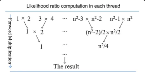
The likelihood ratio function is a multiplication over all the contributions of likelihood ratio area cells. For a scale of n2 array of likelihood ratio area cells with m particles are used, the computing of weight will entailm blocks and resultingn2threads in each block. The value of n2 should be smaller than the maximum number of threads limited by the hardware. Under this condition, the calculating of likelihood ratio in each cell can be parallelized in every thread, but the process of product cannot be parallelized.
In order to alleviate the time complexity caused by the multiplication, the reduction algorithm is adopted in the shared memory of each block to do the product as illustrated in Figure 2. In this way, running time of the multiplication can be reduced significantly. As a result, the time complexity of weight process in PFTBD could beO(log2n) comparing toO(n) without using the shared memory.
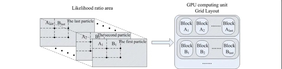
For larger application scenarios, such as in radar appli-cation, the likelihood ratio area includes a 3D array of dimension R × D × B, which always exceeds the max-imum available threads in one block. Thus, some strat-egies must be applied to resolve the massive parallelism
in large scene. According to the number of threads in one block, the likelihood area is divided into small areas as illustrated in Figure 3. The multiplications of each area A1, A2,. . .,Alast are calculated on GPU at the same time and other areas are sequentially calculated. Then the result of the likelihood ratio area is the product of all the small areas.
Obviously, the operations in Figure 3 are complex. From algorithm aspect, Torstensson and Trieb [19] have made a research on different size of likelihood ratio areas in radar application. Its scheme is to use small likelihood ratio areas to obtain the tradeoff between the performance and the extremely high computational cost. In the GPU implementation, we can follow the idea of [19] to sidestep the complex operations discussed above. More specifically, by using likelihood ratio areas with sizes that are just lower than the block, we can obtain better performance but with little computational cost in-crease. The simulations on different size of likelihood ratio areas are given in Section 4.2.
4. Simulation results
4.1. Simulations in infrared scenario
The simulation in infrared scenario is based on the model in [7]. The length of observation time is 30 and a target presents from frames 7 to 21. The observation area is divided into n × m = 20 × 20 cells and the cell size isΔx=Δ=1. The probability of birth and death is Figure 3The programming on GPU for the likelihood ratio area of large scene.
Table 1 Benchmark systems
System 1 System 2 System 3
Software Visual studio 2010 professional with CUDA 4.1 SDK
MATLAB 2010a
Hardware Nvidia GeForce GT9500
Nvidia GeForce 240GT
Pentium(R) Dual-Core E5800 @ 3.20 GHz
32 cores @ 550 MHz
96 cores @ 550 MHz
set as Pb = 0.05 and Pd = 0.05. The initial state of the target is X7 = [4.2 0.45 7.2 0.25 20]T. The SNR is 3 dB. More information about the parameters can be seen in [7]. Various numbers of particles are adopted with each 100 Monte Carlo trials. To verify the effect of different implementation, simulations are performed on three systems, which are given in Table 1.
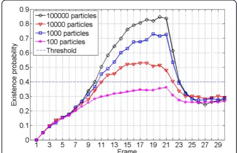
4.1.1. The performances with different numbers of particle The performances of the existence probability and the location error on System 2 with different number of particles are compared in Figures 4 and 5, respectively.
Figure 4 shows that with the increase in the number of particles, the probability of detection improves signifi-cantly. When the number of particle is 100, the exist-ence probability is always below the detection threshold, so the target cannot be detected. However, with 1,00,000 particles, not only the target can be detected faster, but also the detection probability is increased rapidly. With the time accumulation, when the target appears, the
detection probability can eventually reach more than 0.8. Therefore, the number of particles is one of the key factors of the detection performance in PFTBD. From the other side, Figure 5 shows that the location error decreases efficiently with the increase in the number of particles. Note that both the results are consistent with the theory algorithm and have faint difference with the results of System 3, which are not given here for simplicity.
4.1.2. The speedup ratio of GPU to CPU
For larger likelihood region, the parallel computing is more complex and hence GPU achieves higher efficiency than CPU. As the likelihood region reducing, the speedup ratio of GPU to CPU decreases but the processing time on the GPU is still faster than the CPU. A further analysis of the time spent in different part of the algorithm by the hybrid implementation of GPU and CPU is shown in Figure 6.
Figure 6 shows that most of the time is spent on the two kernel: Birth particle(∙ ) and Continue particle(∙ ). Eighty percentage of executive time is cost on GPU. It means that GPU has fully been utilized.
The running time on GT9500, 240GT, and CPU, re-spectively, in different number of particles is given in Figure 7.
From Figure 7, we can find that with the growing number of particles, the speedup ratio between GPUs and CPU improves significantly. Moreover, Figure 7 shows that the speedup ratio of 240GT is quadruple than GT9500. It is consistent with the specifications in Table 1 that 240GT has the number of CUDA cores triple than that in GT9500 and the memory interface width is much larger than that in GT9500.
4.2. The simulation in radar scenario
The simulation in radar scenario is based on the model in [19]. Length of observation time is 30 and target presents from frames 7 to 21. Initially, the range and Doppler cells of particles are uniformly distributed be-tween [85, 90]km, [−0.22, −0.10]km/s inxdirection, and
Figure 5The location error with different number of particles.
Figure 6Relative time spent in different parts of GPU and CPU implementation.
[−0.1, 0.1]km, [−0.10, 0.10]km/s in y direction. The measurements are consisting of Nr × Nd × Nb = 50 × 16 × 1 sensor cells in each time. The initial state of the target is X7 = [89.6 0.2 0 0]T. The SNR is 3 dB. The number of both the birth particles and continue particles is 10,000. More information about the parameters can be seen in [19]. In this simulation, the same benchmark systems with Section 4.1 are used.
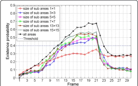
From the algorithm routine in Section 2, we know that there are no remarkable differences in the implementa-tion of PFTBD on GPU between infrared scenario and radar scenario. Here, we emphasize the results for differ-ent size of likelihood ratio areas. The probability of de-tection and the location error with various sizes of likelihood ratio areas on System 2 are given in Figures 8 and 9, respectively.
Figures 8 and 9 show that with the increasing in the size of sub areas, the probability of detection improves and the location error decreases. The simulation results
in the size of sub areas 3 × 3 performs much better than in sub areas of 1 × 1. However, when the size of sub areas extends larger, the existence probability has not improved significantly. From Table 2, we can see that the computational cost is greatly increased as the sub areas increasing in System 3. Nevertheless, in System 2, the increase in running time is so mild for they are all processed in the share memory. Moreover, when the size of sub areas is bigger than 5 × 5, the advantage of the parallelism in GPU can be seen. To our consideration, in the GPU-implemented PFTBD, the size of likelihood areas should be adjusted not only by the application scenario, but also by the amount of share memory on specified hardware.
5. Conclusions
In this article, we propose an efficient implementation of PFTBD algorithm on GPU by CUDA programming. Since the parallel part of the PFTBD algorithm bears the main computation, the running time of the GPU-implemented PFTBD algorithm is greatly reduced by ef-fectively dealing with the particles and the likelihood ratio computations. The implementations are tested on two types of GPU card for the infrared scenario and the radar scenario. As a result, the performance of the GPU-implemented PFTBD algorithm can significantly be improved by employing much more particles in GPU than in CPU.
Figure 8The existence probability with different size of sub areas in radar scenario.
Figure 9The location error with different size of sub areas in radar scenario.
Table 2 Running time for various sub areas compared between systems 2 and 3
Condition Sub areas
1 × 1 3 × 3 5 × 5 7 × 7 13 × 13 15 × 15
System 3 time(s) 3.422 6.070 10.025 16.171 41.322 50.853
System 2 time (s) 10.343 10.436 10.578 10.976 15.972 20.446 Figure 7Time comparison between CPU and GPU with
Competing interests
The authors declare that they have no competing interests.
Acknowledgments
This study was supported by the Fundamental Research Funds for the Central Universities of China (ZYGX2011J012).
Received: 11 December 2012 Accepted: 8 January 2013 Published: 19 February 2013
References
1. B Ristic, S Arulampalam, N Gordon,Beyond the Kalman Filter: Particle Filters, for Tracking Applications(Artech House, Boston, 2004)
2. DJ Salmond, D Fisher, NJ Gordon, Tracking in the presence of spurious objects and clutter, inProceedings of SPIE, Signal and Data Processing of Small Targets, vol. 3373(, Farnborough, Hants, UK, 1998), pp. 460–747 3. MS Arulampalam, S Maskell, N Gordon, T Clapp, A tutorial on particle filters
for online nonlinear/non-Gaussian Bayesian tracking. IEEE Trans Signal Process50(2), 174–188 (2002). doi:10.1109/78.978374
4. DJ Salmond, H Birch, A particle filter for track-before-detect, inProceedings of the American Control Conference. vol. 5 (Arlington, VA, USA, 2001), pp. 3755–3760. doi:10.1109/ACC.2001.946220
5. M Rollason, D Salmond, A particle filter for track-before-detect of a target with unknown amplitude, inProceedings of the IEEE International Seminar on Target Tracking Algorithms and Applications. vol. 1 (QinetiQ, Farnborough, UK, 2001), pp. 14-1–14-4. doi:10.1049/ic:20010240
6. MG Rutten, NJ Gordon, S Maskell, Efficient Particle based track before detect in Rayleigh noise, inProceedings of SPIE, Signal and Data Processing of Small Targets, vol. 5428(Orlando, FL, 2004), pp. 509–519
7. MG Rutten, B Ristic, NJ Gredon, A comparison of particle filters for recursive track-before-detect, inProceedings of the 8th International Conference on Information Fusion. vol. 1 (Piscataway, 2005), pp. 169–175. doi:10.1109/ ICIF.2005.1591851
8. MG Rutten, NJ Gordon, S Maskell, Recursive track-before-detect with target amplitude fluctuations. IEE Proc Radar Sonar Navigat152, 345–352 (2005). doi:10.1049/ip-rsn:20045041
9. Y Boers, JN Driessen, Multitarget particle filter track before detect application. IEE Proc Radar Sonar Navigat151, 351–357 (2004). doi:10.1049/ ip-rsn:20040841
10. The resource for CUDA developers (2010), 2010. http://www.nvidia.com/ object/cuda_home.html
11. Z Shu, C Yanli,GPU Computing for High Performance-CUDA(Beijing, China, 2009) 12. M Bolic, PM Djuric, S Hong, Resampling algorithms and architectures for
distributed particle filters. IEEE Trans Signal Process53(7), 2442–2450 (2005) 13. M Bolic, A Athalye, S Hong, PM Djuric, Study of algorithmic and
architectural characteristics of Gaussian particle filters. J Signal Process Syst
61, 205–218 (2009)
14. C Lenz, G Panin, A Knoll, A GPU-accelerated particle filter with pixel-level likelihood, inInternational Workshop on Vision, Modeling and Visualization (VMV)(Konstanz, Germany, 2008), pp. 235–241
15. G Hendeby, J Hol, R Karlsson, F Gustafsson, A graphics processing unit implementation of the particle filter, inProceedings of the 15th European Statistical Signal Processing(Poznan, Poland, 2007), pp. 1639–1643 16. L Peihua, An efficient particle filter–based tracking method using graphics
processing unit (GPU). J Signal Process Syst68, 317–332 (2012) 17. T Xu, S Jinzhou, Z Fangbin, Particle filter track-before-detect implementation
on GPU, inProceedings of the International Conference on Communications, Signal Processing, and Systems (CSPS)(Beijing, China, 2012), pp. 16–18 18. NVIDIA,CUDA (Compute Unified Device Architecture) C programming guide
4.1, 2011. https://developer.nvidia.com/cuda-downloads
19. J Torstensson, M Trieb,Particle Filtering for Track Before Detect Applications
(University of Linkoping, Sweden, 2005)
doi:10.1186/1687-1499-2013-38
Cite this article as:Tanget al.:Particle filter track-before-detect
implementation on GPU.EURASIP Journal on Wireless Communications and
Networking20132013:38.
Submit your manuscript to a
journal and benefi t from:
7Convenient online submission
7Rigorous peer review
7Immediate publication on acceptance
7Open access: articles freely available online
7High visibility within the fi eld
7Retaining the copyright to your article