Article
1
Predicting Freeway Travelling Time Using Multiple-
2
Source Data
3
Kejun Long1, Wukai Yao2, Jian Gu1*and Wei Wu1
4
1 Hunan Provincial Key Laboratory of Smart Roadway and Cooperative Vehicle-Infrastructure Systems,
5
Changsha University of Science & Technology, Changsha 410004, China; [email protected];
6
[email protected]; [email protected]
7
2 School of Traffic and Transportation Engineering, Changsha University of Science & Technology, Changsha
8
410004, China; [email protected]
9
* Correspondence : [email protected]; Tel.: +86-731-8525-8575
10
11
Abstract: Freeway travelling time is affected by many factors including traffic volume, adverse
12
weather, accident, traffic control and so on. We employ the multiple source data-mining method
13
to analyze freeway travelling time. We collected toll data, weather data, traffic accident disposal
14
logs and other historical data of freeway G5513 in Hunan province, China. Using Support Vector
15
Machine (SVM), we proposed the travelling time model based on these databases. The new SVM
16
model can simulate the nonlinear relationship between travelling time and those factors. In order
17
to improve the precision of the SVM model, we applied Artificial Fish Swarm algorithm to
18
optimize the SVM model parameters, which include the kernel parameter σ, non-sensitive loss
19
function parameter ε, and penalty parameter C. We compared the new optimized SVM model
20
with Back Propagation (BP) neural network and common SVM model, using the historical data
21
collected from freeway G5513. The results show that the accuracy of the optimized SVM model is
22
17.27% and 16.44% higher than those of the BP neural network model and the common SVM model
23
respectively.
24
Keywords: Support Vector Machine; Travelling time; Intelligent Transportation System; Artificial
25
Fish Swarm algorithm; Big data.
26
27
1. Introduction
28
Travel time is one of the main indexes that reflect the traffic operation level of a freeway, and it
29
is also the basis for Advanced Traveler Information System (ATIS), Traffic Guidance System(TGS),
30
and Traffic Control System(TCS). The challenges and difficulties of travel time prediction are
31
identified below.
32
• Diverse influencing factors such as weather, holidays, traffic accidents, out of sample
33
prediction, and mechanisms contributing to congestion. It’s difficult to describe and predict the
34
influence mechanism by using traditional conventional mathematical models.
35
• The complexity and incompleteness of basic data. Although there are many flow detectors and
36
video detection equipment on the freeway, captured data are incompatible, redundant, and
37
include error or loss. To avoid these, techniques which utilize multi-source data to improve the
38
accuracy of travel time prediction is extremely important.
39
In China, practical application of travel time prediction focuses mainly on the following two
40
aspects.
41
The first aspect is the prediction of travel time by map navigation providers using their
42
personalized GPS data. Many map service providers employ their personalized data for travel time
43
forecast services and commercial products. For instance, Bai-du, Gao-de, and other Chinese map
44
providers collect real-time GPS data from users while providing map navigation services. Then, a
45
correlation algorithm is proposed to obtain the travel time prediction result at road sections, which
46
depends on the market share of the map navigation service. The higher frequency of people using
47
the navigation service, the more complete of GPS data and the higher the prediction accuracy will
48
be. However, according to the Chinese market report, the market share of Bai-du and Gao-de
49
services are presently 29.3% and 32.6%respectively. Therefore, the accuracy of results should be
50
further improved by increasing market share.
51
The second aspect is the prediction based on the traffic detection data of urban traffic managers
52
and historical data. In recent years, numerous fixed detector devices have been installed in most of
53
urban roads and rural freeways for the prediction of travel time, including inductive loops, video
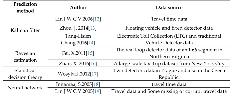
54
recorder, microwave, and laser detection. However, unavoidable damage to flow detection
55
equipment and transmission error of partial data make traffic detection data incomplete redundant
56
or error. In addition, different detectors have different data formats and data accuracy. With the
57
rough use of mistake data for precise travel-time prediction, the Traveler Information Service system
58
cannot recommend optimal travel routes or warn of potential traffic congestion and users cannot
59
determine the optimal departure time or estimate their expected arrival time based on predicted
60
travel times.
61
Theoretical research on freeway travel time prediction can be divided into two categories based
62
on single source data and multi-source data.
63
1.1 Overview ofPrediction Method of Single Source Data
64
A single data source was earlier method used for predict travel time. Many researches
65
prediction results were obtained upon a single data source.
66
Gipps, P. G. [1]used the occupancy and arrival time to predict the travel time in a road in 1997.
67
Mehmet Y, Nikolas G [2]set statistical predictive algorithms to predict the future travel time. Shen,
68
L., &Hadi, M. [3]employed data obtained from detector in freeway. Kyung et al. [4,5]used inductive
69
loop detectors to obtain the front position and capture the interactions between trucks and
70
non-trucks. But fixed detector devices is easily affected by external environment and cannot directly
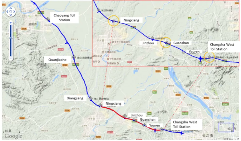
71
access some important parameters, such as travel time, etc.
72
In addition ,many researches consider using GPS data to predict travel time. Ramezani et al. [6]
73
and Zhang et al. [7,8]considered the diversity of GPS data and investigated the application of
74
Markov chain to travel time estimation and implemented good prediction accuracy. Woodard,
75
Nogin &Paul et al. [9]used the GPS data of the current highest volume GPS data source, and applied
76
the TRIP method to predict the travel time. Based on GPS data sets, Bahuleyan, H., &Vanajakshi, L.
77
D. [10] proposed a prediction method for urban trunk lines which was only suitable for traffic
78
conditions in India. But the GPS data only gets the speed and real-time position information and
79
uncertainty due to the route of the vehicle, it affects the coverage and accuracy of detection data.
80
Above methods indeed are innovations and improvements in travel time prediction, and
81
results are more accurate. However, many predictions that use a single data source do not consider
82
the impact of other unexpected events or the result was not accurate enough because single data
83
source cannot reflect traffic state of road network exactly. It will result in certain errors between
84
prediction results and true values.
85
1.2Overview ofPrediction Method of Multiple Source Data
86
Nowadays, the development of traffic big data environment has progressed rapidly. With the
87
support of a large amount of data, it is possible to clearly visualize traffic flow changes under the
88
joint action of different factors, that is, the traffic state presented, which is more favorable. The
89
construction of the predictive model improves the adaptability and accuracy of the model,[11] and if
90
the same state occurs, it can be predicted based on historical results. The more populated the
91
database is, the higher the quality and the higher the likelihood of finding commonalities and
92
predicting accurate results will be. This concept can be applied by searching for common traffic
93
states for prediction.
Owing to progress in the dynamic traffic information acquisition system, various traffic data
95
can be collected more easily. And data fusion is finished in the dynamic traffic information
96
acquisition system, which is jointly determined by the advantages of multi-source data and the
97
characteristics of traffic conditions.
98
And using multi-source data for prediction can overcome the limitations of the single data
99
source. In other words single data source has low quality and is not comprehensive. The traffic state
100
is described from different angles and directions to improve the accuracy of prediction and reduce
101
disturbance from unexpected factors.
102
At present, many studies have been conducted on travel time prediction, especially studies
103
based on the historical data travel time of multi-source data.
104
The common predicting methods and their characters are summarized in the table below.
105
Table 1. Comparison of common prediction methods
106
Prediction
method Author Data source
Kalman filter
Lin J W C V.2006[12] Travel time data
Zhou, J. 2014[13] Floating vehicle and fixed detector data
Tang-Hsien
Chang.2016[14]
Electronic Toll Collection (ETC) and traditional Vehicle Detector data
Bayesian estimation
Fei, X.2011[15] The real loop detector data of an I-66 segment in
Northern Virginia
Zhan, X. 2016[16] A large-scale taxi trip dataset from New York City
Statistical
decision theory Wosyka,J.2012[17]
Two detectors datain Prague and also in the Czech Republic.
Neural network Innamaa, S.2005[18] travel time data
Lin J W C V.2005[19] Travel data and Some missing or corrupt travel data
Compared to the single source data, the multi-source data method can extract deep information
107
within data, significantly reduce the cost of data acquisition, and make up for lack of information
108
and packet loss of single source data. At present, big data application technology are widely used in
109
the traffic field, many studies have been conducted in the field of freeway travel time prediction
110
based on big data analytics. However, there are several deficiencies including:
111
• The method pays attention to machine learning algorithms and lacks the mastery of the
112
characteristics of the traffic flow, resulting in the uncoordinated and unsuitable correspondence
113
between the data and the traffic flow.
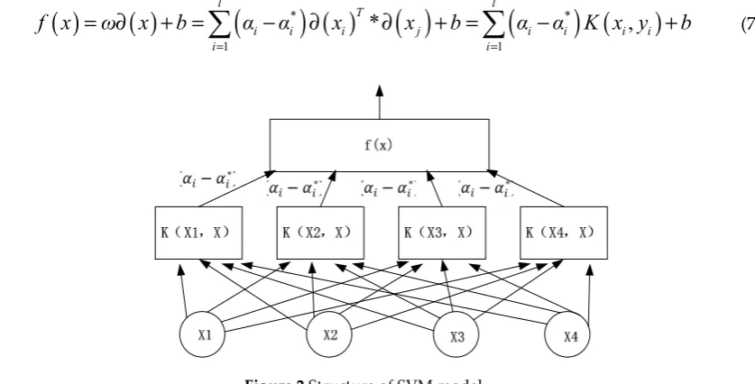
114
• With the continuous updating of big data, it provides conditions for traffic travel time
115
prediction, but some advantages and characteristics of these data are not noticed, resulting in
116
many useful data not being used and mined
117
• Some model parameter calibration is too subjective, which largely depend on researchers'
118
experience;
119
• Some model mostly aimed at a specific example, and cannot be easily adapted to other
120
situations.
121
Therefore, in this study, historical data of a freeway toll station were collected, and were
122
categorized using the support vector machine (SVM) algorithm. Although the predecessors have
123
done some work: Wu, Chun-Hsin[20]used the method of support vector regression to predict the
124
time; Vanajakshi[21] obtained the support vector for short-term prediction of travel time by
125
algorithm. Machine technology; Mendes-Moreira [22]obtained a regression method for comparing
126
long-term travel time prediction through intelligent data analysis. But their analysis is based on
127
machine learning algorithms and does not better understand or improve the transportation system.
128
So this paper uses SVM model based on historical data to predict the common traffic state and the
129
method used for model construction was simplified. The practicability of the prediction algorithm
130
was enhanced to overcome assumptions and uncertainties in the existing traffic flow theory.
2. Data Collection and Preprocessing
132
2.1 Data Description
133
Data for this study was collected in the FreewayG5513 from Changsha to Yiyang, Hunan
134
Province, starting from the Changsha toll station and ending at Yiyang toll station. This freeway
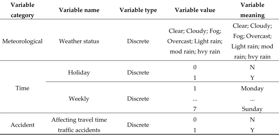
135
G5513 is a standard freeway with a two-way four lane of 100 km/h and a roadbed width of 26 m. The
136
total length was approximately 63 km, the daily average flow reached 58,000 vehicles, and the peak
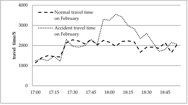
137
flow during long vacation was up to 96,600 vehicles. Because of heavy traffic, the freeway has been
138
rated as one of the six most congested sections in the Hunan Province. There are nine toll stations
139
along the road, from east to west, that is Changsha West, Youren, Guanshan, Jinzhou, Ningxiang,
140
Xiangjiang West, Quanjiao, Chaoyang, and Yiyang North, illustrated as Figure1.
141
142
Figure 1. Layout of the freeway and toll station
143
The main data set collected in this study includes:
144
• Toll data of the whole toll stations along G5513 in February 2018 (vehicles entering and leaving
145
toll station), with a total of 561,081 data items, including the name of the toll station, the time of
146
vehicle entering and leaving the toll station, vehicle type and weight.
147
• Weather information surveying station located near the freeway, which was collected from the
148
Chinese Weather Network in February 2018, with a total of 672 data items, including 24 hour
149
daily weather, temperature, relative humidity, precipitation, and wind direction.
150
• Freeway blockage record statistics, which was obtained from the freeways management
151
department, a total of 260 freeway blockage information reports were collected in February,
152
March, April, and May, including blockage location, reasons for the blockage, blockage start
153
time, and blockage end time.
154
• Freeway traffic control measures report, which was obtained from the Traffic Police
155
Department, with a total of 7 data items collected on April 5 Qingming traditional
156
national Festival, May 1 International Labor Day, and other holiday control information.
157
2.2 Data Preprocessing
158
Many abnormal data items were found in the data, which need to be preprocessed before use.
159
• Data sharing the same entry and exit toll
On the freeway, some drivers turn around in the service area or other sections to avoid the
161
charges and even exchange the toll tags, which is likely to make the entry and exit of the vehicles at
162
toll stations consistent.
163
Therefore, it is necessary to determine whether a data item is consistent with the toll gates and
164
eliminate invalid data items.
165
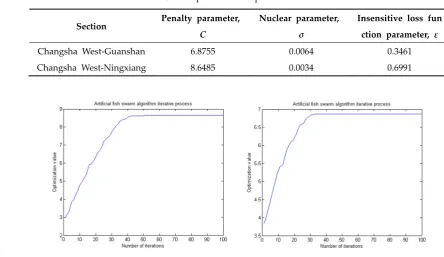
• Abnormal time record data
166
Owing to the failure of the time system associated with toll station to synchronize or system
167
failure, the time of accessing the toll station can be earlier than the time of exiting the toll station. In
168
addition, there are other factors that can lead to long travel time, such as the breakdown of vehicle
169
on road, accidents, and the situation where driver may have a long rest in service area. All of these
170
situations will result in unusual time record data.
171
In the process of data preprocessing, abnormal time data record can be eliminated by screening.
172
• Missing data
173
There are two main reasons for missing data: on the one hand, it’s mainly from equipment
174
problems or road environment includingthe unstable scanning frequency of detector, faulty of
175
transmission equipment, and traffic jam On the other hand, eliminating wrong data items will also
176
lead to partial data missing . Lack of data will cause the road real traffic conditions to change directly
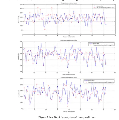
177
or indirectly. Therefore, it is essential to make up for the missing data for historical data. Because of
178
the strong continuity of the traffic flow travel time parameter, the trend in the change of the traffic
179
flow travel time parameter with time is consistent, although its fluctuation will change as the
180
collection period changes. Therefore, the following data fill formula is obtained, as given in equation
181
(1).
182
( )
3
( )
1
2
(
2
)
1
( )
3
6
6
6
data t
= ×
data t
− + ×
data t
− + ×
data t
−
(1)
183
Where, data(t)represents the current missing data, data(t-1), data(t-2) and data(t-3) arethe traffic
184
flow travel time data of the past period, two cycles, and three cycles are respectively represented.
185
3. Support Vector Machine Model
186
3.1 Problem Descriptionof Freeway Travel Time Prediction
187
Travel time of a freeway has strong continuity in a certain time range. That is, there are some
188
complex functional relationships between the current travel time and the past travel time. By
189
analyzing the changes in travel time, we can obtain rules and establish a real-time prediction model
190
updated every 5 min. Then, the accuracy and reliability of the predicted results can be improved by
191
using an optimization algorithm to find the optimal solution of the model.
192
The change in the freeway travel time in different time periods is not a simple linear
193
relationship, and it will neither increase indefinitely, nor decrease indefinitely. But it will only
194
change continuously within a floating interval. Therefore, using a simple least squares regression
195
prediction or similar methods is not sufficient to predict the travel time. The SVM nonlinear
196
regression theory can be employed to solve this problem.
197
SVM uses nonlinear transformation to map the original variables to a high-dimensional feature
198
space, so that the problem of nonlinear separability in the original sample space is transformed into
199
high-dimensional feature space. The linear separable problem and the application of expansion
200
theorem of the kernel function in the calculation process do not require the explicit expression of
201
nonlinear mapping. In addition, since the linear learning machine is established in the
202
high-dimensional feature space, it can be compared to the linear model. The comparison not only
203
increases the complexity of the calculation, but also solves the problem of “dimensional disaster”.
204
Owing to changes in the traffic environment, sudden traffic accidents, weather, and other
205
special events, the SVM algorithm will eventually be transformed into a quadratic programming
206
problem. In theory, a global optimal solution can be obtained, thus solving the traditional neural
207
network. The network can’ avoid the local optimal problem, and should adequately accommodate
the influencing factors due to these sudden changes to improve the accuracy of the travel time
209
prediction result.
210
Therefore, this study used the nonlinear support vector machine regression theory[23].
211
3.2 Model Overview
212
The SVM is a machine learning method, which is based on the statistical learning theory
213
developed by Vapnik. The theory has been further extended to diversified application algorithms,
214
including the linear SVM classification algorithm, the nonlinear SVM classification algorithm, the
215
linear SVM regression algorithm, and the nonlinear SVM regression algorithm[24]. These SVM
216
algorithms have been widely used in many fields owing to their simple structure and high
217
computational efficiency.
218
Consider a training sample set of
i
training samples,{
(
)
}
1
i
,
i i,
i li
S
x y x
R y
R
=
=
∈
∈
, which is219
non-linear, where
x
i is the input column vector of thei
training sample,220
1
,
2,
d T,
i i i i i
x
=
x x
x
y
∈
R
is the corresponding output of the kernel function221
(
i,
i)
( )
i T* ( )
jK x y
= ∂
x
∂
x
.222
Equation (1) in the following is the linear regression equation established in the high
223
dimensional space, and
ε
is introduced as a linear insensitive loss function:224
( )
( )
f x
= ∂
ω
x
+
b
(2)
225
( )
(
)
( )
( )
( )
0,
, ,
,
f x
y
ε
L f x y
ε
f x
y
ε
f x
y
ε
− ≤
=
− −
− >
(3)226
Where,∂
( )
x is the nonlinear mapping function, f x( )
is the prediction function, which returns227
the predicted value, and y is the corresponding real value.
228
Under the above constraints, we can find the optimal classification hyper-plane, that is, find the
229
solution to the following optimization problem.
230
( )
2
2
. .
T,
1, 2, ,
i i
ω
min
s t
ω
x
b y
ε
i
l
∂
+ −
≤
=
(4)231
This problem can be solved by solving the saddle point of the Lagrange function, and its dual
232
theory can be applied to solve the dual problem.
233
(
)(
) (
)
(
)
(
)
(
)
* * * *
1 1 1 1
* *
1
1
,
2
. .
0, ,
0,
1, 2, ,
l l l l
i i j j i j i i i i i
i j i i
l
i i i i
i
min
α
α
α
α
K x x
ε
α
α
y
α
α
s t
α
α
α α
i
l
= = = = =
−
−
+
−
−
−
−
=
≥
=
(5)234
To solve the dual problem, a relaxation factor can be set for each data point. After introducing
235
these two relaxation factors,
ξ
i, ( ,
ξ
i*ξ ξ
i i*≥
0,
i
=
1, 2, , )
l
,the function can be optimized as:236
(
)
( )
( )
2 * 1 *2
. .
,
1, 2 ,
,
. .
,
1, 2 ,
,
l
i i
i T
i i i
T
i i i
ω
m in
C
ξ
ξ
s t
ω
x
b
y
ξ
ε
i
l
s t y
ω
x
b
ξ
ε
i
l
In the above equation, C is the penalty factor; the smaller the value, the smaller the penalty to
238
the error data.
239
Next, the Lagrangian multiplier method can be used to solve the optimization algorithm, and
240
the nonlinear regression function can be further used to solve the double optimization problem.
241
( )
( )
(
*)
( )
( )
(
*)
(
)
1 1
*
,
l l
T
i i i j i i i i
i i
f x
ω
x
b
α
α
x
x
b
α
α
K x y
b
= =
= ∂
+ =
−
∂
∂
+ =
−
+
(7)
242
243
Figure 2.Structure of SVM model
244
For the freeways, there is essentially no significant error in the travel time between the low peak
245
period and even the flat peak period. However, the impact of different traffic conditions on the
246
travel time is inevitable during peak periods. Therefore, the two cases should be discussed
247
separately. Furthermore, whether or not the working day has a different influence on the travel time
248
of vehicles traveling on the highway. The commuting time, travel purpose, and travel mode will be
249
also different. Therefore, these two points should be viewed separately. In addition, road weather
250
conditions and traffic control will have certain influence on the prediction results and should be
251
considered.
252
Based on the SVM model, input workdays, non-working days, the morning and evening peak
253
periods, and off-peak hours as original values, finally can get six time periods: the morning peak
254
hours on workdays, the evening peak hours on workdays, off-peak hours on workdays and so on.
255
Weather and traffic control factors for the four scenarios can also be analyzed. However, the
256
difference in highway traffic conditions between the working day and the non-working day, the
257
morning and evening peak periods and flat peak period is not considered due to the limitation of the
258
length of the article.
259
This study used the travel time prediction of evening peak hours in the classified working
260
days and non-working day peak hours as an example by comparing the traffic data of multiple
261
working days and non-working days.
262
3.3 Model Construction
263
The freeway travel time prediction model is based on the SVM algorithm and is constructed
264
based on the relationship between the current travel time of the road segment and the past travel
265
time of the road segment, the current weather, and the possibility of traffic control.
266
In this study, data from two toll stations with different distances from east to west of G5513
267
were selected for analysis. Moreover, as the first-class passenger car (7 passenger car) accounts for
268
the vast majority of the data, the travel time of the first-class passenger car was taken as the
269
prediction object, and the analysis time interval is 5 minutes.
270
The characteristic of the toll station is presented in table 2.
Table 2. Analysis objects of freeway travel time prediction
273
Toll station Start point End point Distance (kilometer)
1 Changsha West Guanshan 10.6
2 Changsha West Ningxiang 23.2
The structure of the SVM is similar to the neural network. The output is a linear combination of
274
intermediate nodes, and each intermediate node corresponds to a support vector. To determine the
275
optimal classification function, this study takes the four travel times of the time period before the
276
prediction time as the input, namely
t
k−1,t
k−2,t
k−3,t
k−4.277
(
1,
2,
3,
4)
k k k k k
t
=
g t
−t
−t
−t
− (8)278
k is the current time period, and
t
krepresents the average travel time of all vehicles in the279
current predicted time period.
280
In the prediction process, variables such as weather, traffic accident that affects the travel time,
281
holiday or non-holiday, and day of the week, are evaluated as follows:
282
Table 3.Variables type and its meanings
283
Variable
category Variable name Variable type Variable value
Variable
meaning
Meteorological Weather status Discrete
Clear; Cloudy; Fog;
Overcast; Light rain;
mod rain; hvy rain
Clear; Cloudy;
Fog; Overcast;
Light rain; mod
rain; hvy rain
Time
Holiday Discrete 0 N
1 Y
Weekly Discrete 1
...
7
Monday
...
Sunday
Accident Affecting travel time
traffic accidents Discrete
0 N
1 Y
Many traffic accidents occur on the freeway every day. To simplify the parameters, we divide
284
traffic accidents into two categories: traffic accidents that affect the travel time and those that do not.
285
In this study, traffic accidents that affect the travel time was regarded as invariant.
286
The following figure shows a comparison of travel time affected by an accident and normal
287
travel time on the afternoon of February 17.
289
Figure 3. Comparison of accidents and normal travel time
290
Since SVM is a machine learning model, sample training is required before prediction. Multiple
291
groups of any four consecutive travel times, daily weather, traffic accidents that affect the travel
292
time, holidays, and weekday data were used as training samples to obtain a trained model. In the
293
trained model,
t
k−1,t
k−2,t
k−3,t
k−4, weather, accident, holiday, and week are used to predict the294
travel time of the next time period. When a certain number of training samples is achieved, real-time
295
data input can be adopted to predict future results. Moreover, the model can be constantly modified
296
based on the relation between the predicted data and the predicted data to prediction accuracy.
297
3.4 Parameter Calibration and Optimization
298
Parameter selection is very important to find the optimal hyper-plane in the SVM model used in
299
this study. Existing studies mainly adopted the traditional grid search method, direct determination
300
method, one-dimensional search method, and inverse ratio method to determine the insensitive loss
301
function parameter ε and penalty parameter C. However, there are many shortcomings associated
302
with these methods, and the resulting errors will significantly influence the accuracy of the
303
prediction results.
304
Moreover, in the SVM model, kernel function selection is also an important factor that
305
influences the performance of the SVM. The radial basis kernel function
(
,
)
2i
i i
x x
σ
K x y
e
−
=
(RBF) is306
an adaptive kernel function for low-dimensional space data and high-dimensional space, which
307
have good convergence domains, and this function can be described as an ideal kernel function.
308
Therefore, the RBF was selected as the classification prediction kernel function of the SVM, in which
309
a kernel parameterσ needs to be optimized.
310
Therefore, three parameters need to be optimized, namely the core parameter σ, the
311
non-sensitive loss function parameter ε, and the punishment parameter C. The kernel parameter σ is
312
the distribution or range of the training sample data. The non-sensitive loss function parameter ε
313
affects the number of support vectors. The larger the value of ε, the lower the regression precision,
314
and the fewer the support vectors. The penalty parameter C is used to control the degree of
315
punishment of samples beyond the allowable error range. The higher the value, the heavier the
316
punishment of samples.
317
We used the artificial fish swarm algorithm to optimize the parameters of the regression model.
318
The artificial fish swarm algorithm has unique advantages in parameter optimization and
319
overcomes the blindness of traditional algorithms in parameter optimization and the defects of the
320
linear model and neural network in parameter selection. It can be said that the parallel performance
321
of the artificial fish swarm algorithm can ensure that the model parameters converge faster to the
322
global optimization extreme[24,25].
323
0 1000 2000 3000 4000
17:00 17:15 17:30 17:45 18:00 18:15 18:30 18:45
tr
avel
t
im
e/
S
The first step in the optimization process of the artificial fish swarm algorithm is to feed in the
324
training value and the training target through the SVM model to calculate the fitness of the
325
individual. The most adaptable individual is regarded as the optimal value of the current fish group
326
and the corresponding parameters σ, ε, and C of the current optimal value are saved. In the
327
subsequent iteration, σ, ε, and C corresponding to the maximum fitness value are taken as the final
328
optimization results.
329
4. Case Study
330
4.1 Data Selection
331
The data used in this study was collected in February 2018 on G5513 (from Changsha West to
332
Guanshan/Ningxiang Station)in Changsha, Hunan Province, China. The travel time was detected for
333
all days and the detection interval is 5 minutes. Furthermore, 288 sequences are included in one day.
334
The daily evening peak (17:00-19:00) data of G5513 (Changsha West to Guanshan /Ningxiang
335
Station) was selected as an example after comparing data of multiple working days and
336
non-working days, which contains 204 to 228 items. Other variable data items also need to be filtered
337
according to the above data. The dimension feature values are based on the time series and the data
338
requirements according to the prediction model.
339
In this study, the regression SVM model is used to establish the model parameters, and the
340
artificial fish swarm algorithm is used to establish the model parameter optimization algorithm. The
341
optimization results are presented in Table 4. The optimization process for the optimal value of the
342
penalty parameter C is shown in Figure 4.
343
Table 4. Optimization of parameter values
344
Section Penalty parameter, C
Nuclear parameter, σ
Insensitive loss fun ction parameter, ε
Changsha West-Guanshan 6.8755 0.0064 0.3461
Changsha West-Ningxiang 8.6485 0.0034 0.6991
345
346
Figure 4. The parameter optimization curve
347
The parameters of the artificial fish swarm algorithm are set as follows: the maximum number
348
of iterations of the artificial fish is 100; the population size is 5; the maximum number of trials is 5;
349
the crowding factor δ is 0.618; the perceived distance is 0.5; and the moving step is 0.1.
350
4.2 Results and Comparative Analysis
351
The data adopted in this study were obtained during the Chinese Spring Festival from
352
February15 to 21, 2018.Therefore, the data was divided into working days and holidays. There were
336 sets of data from February1 to 14,2018(14 days data) in each group of toll stations; 264 groups (11
354
days) were randomly selected as training data input, and 72 groups (3 days) were adopted as
355
prediction numbers. There were 168 sets of data from February15to 21,2018(11 days data) in each
356
group of toll stations;96 groups (4 days) were randomly selected as training data input, and 72
357
groups (3 days) were adopted as prediction numbers.
358
The detection time is from 17:00 to 19:00 P.M. and the value was taken as test data.
359
BP neural network, SVM, and optimized SVM were used for the prediction. The root mean
360
square error (RMSE), the mean absolute percent error (MAPE) and the covariance protocol (CP)
361
were selected as the error evaluation criteria in the prediction process[26].
362
The RMSE is a comprehensive evaluation indicator of the prediction effect, the MAPE is the
363
prediction relative error, while the CP is the error component analysis indicator.
364
The following figures show the forecasting effect diagram of the holiday evening peak.
365
366
Figure 5.Results of freeway travel time prediction
367
Table 5.Error evaluation of forecasting freeway travel time
368
Method
Changsha West- Guanshan
Station
Changsha West-Ningxiang
Station
RMSE MAPE CP RMSE MAPE CP
Working
day
BP neural
network 7.6544 5.0873 0.5489 10.5124 5.5104 0.5809
Optimized
SVM 6.0369 4.6536 0.5952 8.3069 4.4524 0.6404
Holiday
BP neural
network 11.6308 9.1023 0.5990 16.0845 9.6148 0.6454
SVM 11.5152 7.8645 0.6460 13.3215 8.1153 0.6905
Optimized
SVM 9.6218 6.2451 0.7621 12.2548 7.8651 0.7245
From Table 5, it can be observed that the working day was predicted by the RMSE, the MAPE,
369
and the CP data between the two toll stations. It could be found that all three models can be used for
370
predicting travel time.
371
Although the prediction error of the BP neural network may be larger than those of the SVM
372
and the optimized SVM models, there is no deviation between the error of the SVM and the
373
optimized SVM model.
374
However, when forecasting holidays with large traffic and long travel time, the RMSE of the
375
optimized SVM model is significantly better than those of the BP neural network and the SVM
376
model.
377
In the prediction of Changsha West-Guanshan, the accuracy of the optimized SVM model using
378
artificial fish swarm algorithm is 17.27% higher than that of the BP neural network model and
379
16.44% higher than the conventional SVM model.
380
In the prediction of Changsha West-Ningxiang, the accuracy of the optimized SVM model
381
using artificial fish swarm algorithm is 23.80% and 8.01% higher than those of the BP neural network
382
model and the conventional SVM model, respectively.
383
The optimized SVM model described in this paper has higher travel time prediction accuracy in
384
the road segment, and the mapping law of the input and output are better represented by the
385
optimized SVM model.
386
In terms of the relative prediction errors of the three prediction models, the MAPE of the
387
optimized SVM model is lower than the prediction errors of the BP neural network and the
388
conventional SVM model when using holiday and working day data. This indicates that the
389
optimized SVM model described in this paper has certain advantages in terms of the travel time
390
prediction model of the road segment, and the data requirements are lower.
391
4.3 Analysis of Influencing Factors of Travel Time
392
The freeway travel time is determined by various factors, such as weather, traffic accident,
393
holiday, and week day. However, owing to limitations of sample data, only traffic accidents and
394
holidays were considered.
395
4.3.1 Effect of traffic accidents on travel time
396
First, the optimized SVM model described in this paper is superior to the BP neural network
397
and SVM model in terms of the CP.
398
In the prediction of Changsha West-Guanshan, the CP of the optimized SVM model is 21.40%
399
higher than that of the BP neural network model, which is 7.28% higher than that of the conventional
400
SVM model;
401
In the prediction of Changsha West-Ningxiang, the CP of the optimized SVM model is 10.9%
402
and 6.53% higher than those of the BP neural network model and the conventional SVM model,
403
respectively.
404
The results presented in this paper indicates that the optimized SVM model has better
405
inclusiveness and stability when unexpected factors such as traffic accidents that affect the travel
406
time are encountered, thereby avoiding the need for repeated trial and error to address network
407
problems.
Second, freeway traffic accidents will cause the traffic capacity of certain sections of the road
409
network to decrease, and queues will be formed near the accident site, which increases the travel
410
time of the vehicle.
411
4.3.2 Effect of holidays on travel time
412
A comparison of the working day and holiday forecasting error evaluation criteria presented in
413
the previous section indicates that the BP neural network has a larger prediction error than the
414
working day prediction results of the other models probably due to the problem of construction of
415
the network structure. However, the conventional SVM and the optimized SVM models have similar
416
prediction error results. In the above analysis, there are large gaps in the holiday prediction results
417
of the three different models.
418
It can observed that holidays have significant influence on the travel time. The effect of holidays
419
on the travel time, which was obtained from the analysis of the original toll station data, is that it
420
significantly increases the volume of traffic on the highway network.
421
5. Conclusions
422
This study performed an in-depth analysis of freeway travel time prediction to provide
423
high-quality travel experience for users and found that the freeway travel time is affected by travel
424
time, weather, and traffic. The effect of different factors was analyzed, such as accidents and
425
holidays.
426
Bad weather reduces the overall traffic rate, which increases the travel time. Traffic accidents
427
lead to reduced road traffic capacity, which affects the travel time. Free passage on highways during
428
holidays and the increased demand for travel result in increased vehicle flow, which also affects the
429
travel time.
430
In this study, basic data was analyzed, and the traffic state prediction method based on SVM
431
data mining technology was proposed to transform the problem into a quadratic programming
432
problem using artificial fish swarm algorithm, which reduces the computational and local optimal
433
problems of traditional neural networks. The parameters of the SVM were optimized using
434
traditional network optimization, and a global optimal solution was obtained.
435
Results show that the accuracy of the optimized SVM model is 17.27% and 16.44% higher than
436
those of the BP neural network model and the conventional SVM model, respectively. Accurate
437
prediction of the travel time on the freeway was realized, which can provide data support for
438
monitoring, early warning, and decision analysis for the freeway operation status.
439
In this study, influencing factors such as weather, traffic, accidents and holidays were included
440
in the optimization of the SVM prediction model. However, owing to limitations of the number of
441
samples, the model was not fully trained. Therefore, a certain error occurred in the prediction
442
results.
443
In the future, it is necessary to categorize traffic accidents, clarify the impact of each type of
444
accident on the travel time, categorize increase in the holiday traffic, and clarify the impact of each
445
level of accident on the travel time. Furthermore, the number of training samples, database capacity,
446
and prediction accuracy should be continuously increased. In this study, only data from freeway toll
447
stations was validated, and application to actual large-scale road networks should be further
448
explored in the future.
449
450
Author Contributions: This work was conducted by Kejun Long and Wei Wu with the help of graduate
451
student Wukai Yao. It was mainly drafted by Kejun Long and Wukai Yao, and checked and revised by Wei
452
Wu and Jian Gu. Kejun Long and Wukai Yao designed and analyzed the proposed model. Wukai Yao and Jian
453
Gu performed the simulation. Kejun Long is responsible for the English polish and proofreading of the work.
454
Funding: This research was funded by National Natural Science Foundation of China (NSFC),grant number
455
51678076, Hunan Provincial Key Laboratory of Smart Roadway and Cooperative Vehicle-Infrastructure
456
Acknowledgments: The authors express their thanks to all who participated in this research for their
458
cooperation. The authors would like to give great thank to the hard work by the peer reviewers and editor.
459
Conflicts of Interest: The authors declare no conflict of interest.
460
References
461
1. Gipps,P.G. The estimation of a measure of vehicle delay from detector output. Newcastle-Upon-Tyne
462
University, England1977, 18 p.
463
2. Yildirimoglu, M; Geroliminis, N. Experienced travel time prediction for congested freeways. Transp. Res.
464
Part B-Method, 2013, 53(4):45-63.
465
3. Shen,L; Hadi,M. Practical approach for travel time estimation from point traffic detector data. J. Adv
466
Transportation, 2013, 47(5):526-535.
467
4. Hyun ,K; Tok,A, Ritchie S G. Long distance truck tracking from advanced point detectors using a selective
468
weighted Bayesian model. Transport. Res. Part C-Emerg. Technol, 2016, 82:24-42.
469
5. Hyun, K. K.; Jeong, K. Assessing crash risk considering vehicle interactions with trucks using point
470
detector data. Accid. Anal. Prevent, 2018, 17p.
471
6. Ramezani, M.; Geroliminis, N. On the estimation of arterial route travel time distribution with Markov
472
chains. Transp. Res. Part B, 2012, 46(10): 1576-1590.
473
7. Zhang, J. T.; Zhou, J. An Arterial Travel Time Estimation Model Based on Discrete Time Markov Chains.
474
Syst. Eng, 2014,5:98-104.
475
8. Zhang, J. T.; Zhou, J. Travel time estimation model based on spatial Markov chains. Syst. Eng,2015,12
476
:72-77.
477
9. Woodard, D.; Nogin,G. Predicting travel time reliability using mobile phone GPS data. Transport. Res.
478
Part C-Emerg. Technol, 2017, 75:30-44.
479
10. Bahuleyan, H.;Vanajakshi, L. D. Arterial path-level travel-time estimation using machine-learning
480
techniques. J. Comput. Civil. Eng, 2016, 31(3), 04016070.
481
11. Tan, Y. Current Situation of Short-term Flow Forecasting and Discussion on Forecasting Method in Big
482
Data Environment. ITS China:2017:10.
483
12. Lin J W C V. Incremental and online learning through extended kalman filtering with constraint weights
484
for freeway travel time prediction. ITSC. IEEE, 2006:1041-1046.
485
13. Zhou, J.; Zhang, C.B. Travel Time Prediction Model for Urban Road Network based on Multi-source Data.
486
Procedia - Social and Behavioral Sciences, 2014,138.
487
14. Tang-Hsien Chang; Albert Y. Chen. Freeway Travel Time Prediction Based on Seamless Spatio-temporal
488
Data Fusion: Case Study of the Freeway in Taiwan. Transportation Research Procedia,2016,17.
489
15. Fei X; Lu C C. A Bayesian dynamic linear model approach for real-time short-term freeway travel time
490
prediction. Transp. Res. Part C, 2011, 19(6):1306-1318.
491
16. Zhan, X.; Ukkusuri, S. V. A Bayesian mixture model for short-term average link travel time estimation
492
using large-scale limited information trip-based data. Autom.Constr,2016, 72, 237-246.
493
17. Wosyka,J; Přibyl, P. Real-time travel time estimation on highways using loop detector data and license
494
plate recognition. Elektro. IEEE, 2012:391-394.
495
18. Innamaa, S. Short-Term Prediction of Travel Time using Neural Networks on an Interurban Highway.
496
Transportation, 2005, 32(6):649-669.
497
19. Lint, J.W.C.V; Hoogendoorn, S P. Accurate freeway travel time prediction with state-space neural
498
networks under missing data. Transp. Res. Part C, 2005, 13(5):347-369.
499
20. Wu, Chun-Hsin; Jan-Ming Ho. Travel-time prediction with support vector regression.
500
IEEE.Trans.Intell.Transp.Systems.5.4 ,2004: 276-281.
501
21. Vanajakshi, L; Rilett, L R. Support Vector Machine Technique for the Short Term Prediction of Travel
502
Time. Intelligent Vehicles Symposium. IEEE, 2007:600-605.
503
22. Mendes-Moreira, João. Comparing state-of-the-art regression methods for long term travel time
504
prediction. Intell. Data. Anal. 16.3 (2012): 427-449.
505
23. Wang, X.;Chen, X. H.; Yang, X. M. Short term prediction of expressway travel time based on k nearest
506
neighbor algorithm.Chin.J.Highw.Transport,2015,28(1), 102-111.
507
24. Li, S.; Yuan, Z. C.; Wang, C. Optimization of support vector machine parameters based on group
508
25. Wang, Q.; Liu, Z.; Peng, Z.A PSO-SVM Model for short-term travel time prediction based on Bluetooth
510
Technology. J. Harbin. Inst. Technol, 2015,22(3), 7-14.
511
26. Yang, Z. S. Study on the Synthetic Link Travel Time Prediction Model of Key Theory of