Comprehensive Water Quality Indexing Using Functional Data and Principal Component Analysis for River Narmada

Comprehensive Water Quality

Indexing Using Functional Data and

Principal Component Analysis for

River Narmada

Swati Mishra

Department of Civil Engineering

Comprehensive Water Quality Indexing

using Functional Data and Principal

Component Analysis for River Narmada

Dissertation submitted in partial fulfillment

of the requirements of the degree of

Master of Technology

in

Civil Engineering

by

Swati Mishra

(Roll Number: 214CE4467)

based on research carried out

under the supervision of

Prof. Kanhu Charan Patra

May, 2016

Department of Civil Engineering

ii

Department of Civil Engineering

National Institute of Technology Rourkela

April 20, 2016

Certificate of Examination

Roll Number: 214CE4467

Name: Swati Mishra

Title of Dissertation: Comprehensive Water Quality Indexing using Functional Data and Principal Component Analysis for River Narmada.

We the below signed, after checking the dissertation mentioned above and the official record book (s) of the student, hereby state our approval of the dissertation submitted in partial fulfillment of the requirements of the degree of Master of Technology in Civil Engineering at National Institute of Technology Rourkela. We are satisfied with the volume, quality, correctness, and originality of the work.

Prof. Kanhu Charan Patra Supervisor

iii

Department of Civil Engineering

National Institute of Technology Rourkela

Prof. Kanhu Charan Patra

Professor

May 28, 2016

Supervisors’ Certificate

This is to certify that the work presented in the dissertation entitled Comprehensive Water Quality Indexing using Functional Data and Principal Component Analysis for River Narmada submitted by Swati Mishra, Roll Number 214CE4467, is a record of original research carried out by him under our supervision and guidance in partial fulfillment of the requirements of the degree of Master of Technology in Civil Engineering. Neither this dissertation nor any part of it has been submitted earlier for any degree or diploma to any institute or university in India or abroad.

Kanhu Charan Patra

Dedication

This dissertation is dedicated to the researchers who work day and night for the well-being of the society…

v

Declaration of Originality

I, Swati Mishra, Roll Number 214CE4467 hereby declare that this dissertation entitled Comprehensive Water Quality Indexing using Functional Data and Principal Component Analysis for River Narmada presents my original work carried out as a post-graduate student of NIT Rourkela and, to the best of my knowledge, contains no material previously published or written by another person, nor any material presented by me for the award of any degree or diploma of NIT Rourkela or any other institution. Any contribution made to this research by others, with whom I have worked at NIT Rourkela or elsewhere, is explicitly acknowledged in the dissertation. Works of other authors cited in this dissertation have been duly acknowledged under the sections “Reference”. I have also submitted my original research records to the scrutiny committee for evaluation of my dissertation.

I am fully aware that in case of any non-compliance detected in future, the Senate of NIT Rourkela may withdraw the degree awarded to me on the basis of the present dissertation.

May 27, 2016

Swati Mishra

Acknowledgment

“Continuous effort- not strength nor intelligence- is the key to unlocking our potential”, says Winston Churchill.

Getting a seat at National Institute of Rourkela was not easy and nor was sustaining it. The journey of my Masters at the institute has been smooth only because it was geared by my supervisor Prof. K.C. Patra. Like a father, he constantly guided, scolded and corrected me. I would like to thank our External Examiner Prof. R.K. Panda, who, in spite of his busy schedule, stayed at Rourkela and authentically commented and corrected my mistakes. I express my heartfelt gratitude to the other faculty members of Civil Engineering Department who invested their precious time in our coursework and made me aware about the upcoming technologies in Water Resources Engineering.

This is perhaps the first time that I have stayed so far away and for such a long time away from home. My parents have continuously supported me, surprised me and reprimanded me for my wrong doings. I would like to thank my brother who has been a constant light of support at the institute.

My project would have been a dismantled piece of writing had Mrs. Mrunmayee Manjari Sahoo and Mr. Janaki Ballav Swain, both PhD Scholars at the institute, not directed me towards the research and constantly scrutinized my work. It is because of them that the work has been completed in time and has been worthy of the institute.

I thank all my friends who have been with me in this journey for making it an enjoyable one.

May 27, 2016 Swati Mishra

NIT Rourkela Roll Number: 214CE4467

vii

Abstract

The degrading water quality status of River Narmada can be deciphered by a tool called Water Quality Indexing. From the entire river basin seven important sites are chosen. Water Quality pertaining to twenty-five parameters are analyzed from 1991-2013. The final results are averaged to get the indices for a typical year. The current study commences with some preliminary methods. A significance test is conducted to determine three relevant parameters from each site. Based on these relevant parameters, Water Quality Indexing is done using Functional Data Analysis and Principal Component Analysis and finally error analysis of the methods is done. The preliminary analysis show that Biochemical Oxygen Demand, Dissolved Oxygen, Chemical Oxygen Demand and Total and Faecal Coliform are the most crucial water quality variables along the mainstream of Narmada River Basin. Both Principal Component Analysis and Factor Analysis yield seven components from which it is concluded that agricultural runoff and industrial wastes account for an increase in alkalinity in the river water. It is also concluded that the deterioration in Dissolved Oxygen is being rejuvenated by variables causing alkalinity in water.

Conventional Water Quality Indexing done along the seven sites shows that for Station 1,2,5,6 and 7, water quality remains excellent almost throughout the year except for Stations 2 and 4. Functional Data Analysis and Principal Component Analysis also shows similar results. From the error analysis Functional Data Analysis using Entropy Weights is found to have least error.

Thus for a typical year the minimum indices implying the worst water quality are shown in a map which can help in deciphering the water quality status of the river well.

Keywords: Water Quality Indexing; Functional Data Analysis; Entropy Weights; Relative Pollution Degree; Student’s t-test; Principal Component Analysis

Contents

Certificate of Examination ii Supervisors’ Certificate iii

Dedication iv Declaration of Originality v Acknowledgment vi Abstract vii List of Figures ix List of Tables x 1 Introduction 1 1.1 General 1

1.2 Initiation of Water Quality Indices (WQIs) 2 1.3 More on Benefits of Water Quality Indices 3 1.4 Conventional Water Quality Indices Used in Indian

Rivers

3 1.5 Functional Data Analysis 4 1.6 Multivariate Analysis 4 1.7 Problem Statement 5

1.8 Thesis Outline 5

2 Literature Review 6

2.1 Regarding Study Area 6 2.2 Regarding Functional Data Analysis 8 2.3 Regarding Multivariate Analysis 10 2.4 Regarding Water Quality Indexing 12 3 Study Area and Data Collection 14

3.1 General 14

3.1.1 The River Course and Physiography 15 3.1.1.1 Stations selected for study 16 3.1.2 The Climate and Rainfall 17 3.1.3 Water Quality of Mainstream Narmada River

Basin

17 3.2 Data Collection and Analysis 18 3.2.1 Discharge (in cubic metres per second) 18 3.2.2 Temperature (in Degrees Celsius) 19

3.2.3 pH 20

3.2.4 Electrical Conductivity (in micro mho/cm) 21 3.2.5 Total Dissolved Solids (in micro mho/cm) 22 3.2.6 Ammonia Ion Concentration (in mg N/L) 23 3.2.7 Nitrate and Nitrite Ion Concentration in mg N/L 23

3.2.8 Silicon Dioxide (in mg/L) 24 3.2.9 Dissolved Oxygen (in mg/L) 25 3.2.10 Biochemical Oxygen Demand (in mg/L) 26 3.2.11 Chemical Oxygen Demand (in mg/L) 26 3.2.12 Phenol Ions Concentration (in mg/L) 27 3.2.13 Total Alkalinity (in mg CaCO3/L) 28

3.2.14 Total Hardness (in mg CaCO3/L) 29

3.2.15 Calcium Hardness (in mg CaCO3/L) 30

3.2.16 Fluoride Ion Concentration (in mg/L) 30 3.2.17 Calcium Major Ion Concentration (in mg/L) 31 3.2.18 Magnesium Ion Concentration (in mg/L) 31 3.2.19 Sodium Ion Concentration (in mg/L) 32 3.2.20 Potassium Ion Concentration (in mg/L) 33 3.2.21 Chloride Ion Concentration (in mg/L) 33 3.2.22 Sulphate Ion Concentration (in mg/L) 34 3.2.23 Carbonate Ion Concentration (in mg/L) 35 3.2.24 Bicarbonate Ion Concentration (in mg/L) 35 3.2.25 Total Coliform Count (in MPN/100mL) 36 3.2.26 Faecal Coliform Count (in MPN/100mL) 37

4 Methodology 38

4.1 Water Quality Index 38 4.1.1 Parameter Selection 38 4.1.1.1 Student’s t-test 39 4.1.2 Conversion of parameters of different units into a

common scale

40 4.1.2.1 Development of Sub-Indices 41 4.1.2.2 Various Types of Sub-Indices 42 4.1.3 Assigning Weights to the Sub-Indices 42 4.1.3.1 Information Entropy Method 43 4.1.3.2 Relative Pollution Degree 44 4.1.4 Sub-Indices Aggregated to Form the Final Index 45 4.1.4.1 Linear Sum Index 45 4.1.4.2 Weighted Sum Index 45 4.2 Functional Data Analysis 46 4.3 Multivariate Statistics 47 4.3.1 Principal Component Analysis 47 4.3.2 Principal Factor Analysis 48 4.3.4 Cluster Analysis 49 4.4 Miscellaneous Methodologies 50 4.5 Permissible Water Quality Criteria 51 5 Results and Discussions 54 5.1 Preliminary Analysis 54 5.1.1 Descriptive Statistics 54

5.1.2 Principal Component and Principal Factor Analysis

55 5.1.2.1 Correlation Matrix 55 5.1.2.2 KMO-Sampling Adequacy 58 5.1.2.3 Total Variance Explained 58 5.1.2.4 Principal Component Matrix 59

5.1.2.5 Scree Plot 61

5.1.2.6 Rotated Factor Matrix 61 5.1.2.7 Cluster Analysis 63

5.2 Student’s t-test 64

5.3 Conventional Water Quality Indexing 64 5.4 Water Quality Indexing Using Functional Data Analysis 65 5.4.1 Development of Sub-Index Curves 66 5.4.2 Assignment of Weights 70 5.4.2.1 Conventional Weights 70 5.4.2.2 Assignment of Weights by Information Entropy

Method

70 5.4.2.3 Assignment of Weights by Relative Pollution

Degree

74 5.4.2.4 Development of Water Quality Index Curves 78 5.5 Water Quality Index Based on Principal Component Analysis 83

5.6 Error Analysis 88

6 Conclusions 90

7 References List of Figures

Figure 3.1 Location of Study Area

Figure 3.2 Variation of discharge for a typical year 19 Figure 3.3 Variation of temperature for a typical year 20 Figure 3.4 Variation of pH for a typical year 21 Figure 3.5 Variation of Electrical Conductivity for a typical

year

22 Figure 3.6 Variation of Total Dissolved Solids for a typical year 22 Figure 3.7 Variation of Ammonia for a typical year 23 Figure 3.8 Variation of Nitrate and Nitrite for a typical year 24 Figure 3.9 Variation of Silica for a typical year 25 Figure 3.10 Variation of Dissolved Oxygen for a typical year 25 Figure 3.11 Variation of BOD for a typical year 26 Figure 3.12 Variation of COD for a typical year 27 Figure 3.13 Variation of Phenol Ions for a typical year 28 Figure 3.14 Variation of Total Alkalinity for a typical year 28 Figure 3.15 Variation of Total Hardness for a typical year 29 Figure 3.16 Variation of Calcium Hardness for a typical year 30 Figure 3.17 Variation of Fluoride Ions for a typical year 30 Figure 3.18 Variation of Calcium Major Ions for a typical year 31 Figure 3.19 Variation of Magnesium Ions for a typical year 32 Figure 3.20 Variation of Sodium Ions for a typical year 32

Figure 3.21 Variation of Potassium Ions for a typical year 33 Figure 3.22 Variation of Chloride Ions for a typical year 34 Figure 3.23 Variation of Sulphate Ions for a typical year 34 Figure 3.24 Variation of Carbonate Ions for a typical year 35 Figure 3.25 Variation of Bicarbonate Ions for a typical year 36 Figure 3.26 Variation of Total Coliform for a typical year 36 Figure 3.27 Variation of Faecal Coliform for a typical year 37 Figure 4.1 Typical t-distribution curve 40 Figure 4.2 Mechanism of Water Quality Indexing 41 Figure 5.1 A Scree Plot of Eigen Values versus Components 61 Figure 5.2 Dendogram obtained using Hierarchical Clustering 63 Figure 5.3 Average Sub-Index Curves for Station 1 66 Figure 5.4 Average Sub-Index Curves for Station 2 67 Figure 5.5 Average Sub-Index Curves for Station 3 67 Figure 5.6 Average Sub-Index Curves for Station 4 68 Figure 5.7 Average Sub-Index Curves for Station 5 68 Figure 5.8 Average Sub-Index Curves for Station 6 69 Figure 5.9 Average Sub-Index Curves for Station 7 69 Figure 5.10 Entropy Weight Curves for Station 1 71 Figure 5.11 Entropy Weight Curves for Station 2 71 Figure 5.12 Entropy Weight Curves for Station 3 72 Figure 5.13 Entropy Weight Curves for Station 4 72 Figure 5.14 Entropy Weight Curves for Station 5 73 Figure 5.15 Entropy Weight Curves for Station 6 73 Figure 5.16 Entropy Weight Curves for Station 7 74 Figure 5.17 Relative Pollution Weight Curves for Station 1 75 Figure 5.18 Relative Pollution Weight Curves for Station 2 75 Figure 5.19 Relative Pollution Weight Curves for Station 3 76 Figure 5.20 Relative Pollution Weight Curves for Station 4 76 Figure 5.21 Relative Pollution Weight Curves for Station 5 77 Figure 5.22 Relative Pollution Weight Curves for Station 6 77 Figure 5.23 Relative Pollution Weight Curves for Station 7 78 Figure 5.24 Water Quality Index Curves for Station 1 79 Figure 5.25 Water Quality Index Curves for Station 2 79 Figure 5.26 Water Quality Index Curves for Station 3 80 Figure 5.27 Water Quality Index Curves for Station 4 81 Figure 5.28 Water Quality Index Curves for Station 5 81 Figure 5.29 Water Quality Index Curves for Station 6 82 Figure 5.30 Water Quality Index Curves for Station 7 83 Figure 5.31 Water Quality Index Curves for Station 1 using

PCA

84 Figure 5.32 Water Quality Index Curves for Station 2 using

PCA

84 Figure 5.33 Water Quality Index Curves for Station 3 using

PCA

85 Figure 5.34 Water Quality Index Curves for Station 4 using 86

PCA

Figure 5.35 Water Quality Index Curves for Station 5 using PCA

86 Figure 5.36 Water Quality Index Curves for Station 6 using

PCA

87 Figure 5.37 Water Quality Index Curves for Station 7 using

PCA

88 Figure 5.38 Minimum Water Quality Indices for River

Narmada

89

List of Tables

Table 3.1 Description of the stations studied

Table 4.1 Permissible and Acceptable Limits of Water Quality Parameters

51 Table 5.1 Descriptive Statistics for the span 2009-2013 54 Table 5.2 Correlation Matrix 56 Table 5.3 KMO and Bartlett’s Test 58 Table 5.4 Total Variance Explained 59 Table 5.5 Principal Component Matrix 60 Table 5.6 Rotated Factor Matrix 62 Table 5.7 p-values for Student’s t-test 64 Table 5.8 Conventional Indices for a typical year 65 Table 5.9 Different Classes of water with their notations 65 Table 5.10 Stationary Weights of Significant Variables 70 Table 5.11 Error Analysis of the Water Quality Index Methods 88

1

CHAPTER I

INTRODUCTION

Water is an indispensable natural resource. It has played a crucial role in the triggering and sustenance of civilizations. However, till 1960s, extraction of water was more important than its quality assessment. The last three decades of the twentieth century have witnessed the importance of water quality in an alarming rate (Abbasi et.al. 2012).

The water quantity of a resource is defined by the mass of water contained in it. On the other hand, water quality has different constraints according to its use. The water required for household purpose varies from that invested in industries. Different animals require different levels of water quality; same goes with different crops. Thus, water quality depends on anything and everything that it might have gathered during its travel from clouds to the surface or water body; in any form, be it dissolved, colloidal or suspended. The tag of being a “Universal Solvent” expands the canopy of its miscibility.

The quality of water can be described by listing out the concentration of all the chemicals present in a sample. But, such an assessment would be too lengthy depending on the constituents present and would be correctly deciphered by technical experts only.

The question also arises of how to compare two samples having different chemical constituents. The danger of consuming a sample with five components having 5% more concentration than the permissible limit (and hence objectionable): pH, Electrical Conductivity, Hardness, Sodium and chloride may not be equivalent to a sample containing at least 1 MPN of Coliform Count.

2

Thus all the constituents present in a sample should be addressed differently but depicted under a single value. Water Quality Indices solve the vexing problem of quality assessment by following the same formula. They translate the constituents and their corresponding concentrations into a single value on the basis of a system.

The concept of using indices to represent a system is not a novel idea. Be it Dow Jones Index of New York or Sensex of stock exchange of Mumbai, indices have already reserved their place in the field of economics, trade and commerce. Even in ecology, indices have been thoroughly implemented through Shannon Index, Simpson Index and so on.

Thus, indices compositely represent a condition deduced by combining, in several ways, a number of relevant yet incommensurate measurements. This aggregation results in an ordinal number which assists in understanding and inferring the overall contribution of the measurements to the number.

Water Quality Index is an important component of environmental indices. It is used as communication tool by regulatory boards to describe the ‘health’ of any environment system; water, air, sediments or soil. It also helps in the evaluation of various regulatory policies on the different environmental practices.

1.2Initiation of Water Quality Indices (WQIs)

The concept of water quality assessment had its first introduction in Germany in 1848. There, the water was considered fit or otherwise based on the presence or absence of some organisms. Since then European countries have used different classification systems for assessing water quality in their regions. There are two types of classification systems: one concerned with the

3

amount of pollutants present and the other concerned with the number of living communities (macroscopic or microscopic) of organisms present.

These classification systems grouped water bodies into different pollution classes. Unlike this, indices assign a numerical value to represent the condition of water quality of a water body. The use of such a numerical scale begins with Horton’s Index in 1965.

1.3More on the benefits of Water Quality Indices

The use of indices are well-entrenched by the regulatory agencies which are responsible for checking the status of water pollution. After the development of Water Quality Indices, they are further implemented to examine trends, showcase the environmental conditions and evaluate the potential of the regulatory measures of the government. The other uses of water quality indices are resource allocation, R&D, ranking of allocations and environmental planning.

The water quality indices can also be classified into two categories; indices based on physico-chemical parameters and indices based on bioassessment. Usually water quality indices belong to the category based on physico-chemical parameters, including Horton’s Index which includes coliforms as a variable. The present study is also classified under physico-chemical parameters.

1.4Conventional Water Quality Indices Used in Indian Rivers

The first water quality index developed in India and perhaps in Asia too, is developed by Bhargava in 1983 and 1985. This method sub-divides the water quality variables into four groups namely, bacterial group, toxicants, physical and non-toxic parameters. A multiplicative

4

aggregation is used to combine the sub-indices obtained from different functions. This method has been applied to River Yamuna at New Delhi.

An index system, based on National Sanitary Foundation-Water Quality Index, is developed exclusively for River Ganga by Ved Prakash et.al from 2000 to 2010.

In 1995, Dhamija and Jain have used nine water quality parameters to summarize the water quality of Hanuman Lake at Jabalpur.

Sargaonkar and Deshpande in 2003, have developed “Overall Index of Pollution” to evaluate the surface water quality of Indian Rivers.

Swamee and Tyagi in 2000 and 2007 have improved the expressions of sub-indices and aggregation methods for conveying the water quality.

1.5Functional Data Analysis

A branch of statistics and developed by Ramsay (1997), Functional Data Analysis, is a method which works on information represented by functions varying over a continuum, usually time. For this, the sampling data need not be identical and may have missing values. This highly flexible dynamic method has been thoroughly used in the fields of medicine, economy and ecology. A detailed account of this method is given in the further chapters.

1.6Multivariate Analysis

This statistical method involves the observation and analysis where more than one variables occur as outcomes. The techniques used in the present study are Principal Component Analysis, Factor Analysis, Clustering, Discriminant Analysis and MANOVA. These methods have been explained later.

5

1.7Problem Statement

The lifeline of Madhya Pradesh and one of the major rivers of India, Narmada, is being readily polluted by municipal wastes, anthropogenic sewage and industrial wastes. As a result, the water quality has deteriorated to Category ‘B’ i.e. ‘Fit for Outdoor Bathing’ along the river. Hence to create awareness among the people using its water is necessary. Water Quality Indexing is such a technique with which common people can understand the water quality status of a water body. Conventional and Modern Methods of Water Quality Indexing are used in the current research. The objectives of the research are as follows:

i) Applying a Conventional WQI method to the river.

ii) Apply WQI method based on Functional Data Analysis and Modern Statistical Techniques.

iii) Compute the Final Indices along the Mainstream of the River after comparison. iv) Predict the Water Quality Using Clustering and MANOVA.

1.8Thesis Outline

Chapter I acquaints one about the origin of Water Quality Indices and highlights about the methods to be used. The problem statement has been elaborated in this chapter

Chapter II reflects the work done by researchers in the study area and the methods used. It also brings out a critical review of the past works.

Chapter III narrates in detail about the study area, the water quality variables used and their variations in a typical year.

Chapter IV describes about the methodologies incorporated in the research. Chapter V comprises of the results obtained from the research.

6

CHAPTER II

LITERATURE REVIEW

2.1 Regarding Study Area

Ahmad et.al (2001) state that the water quality of many rivers like the Ganges, the Sutlej, the Cauvery, Sabarmati, Krishna, Khan-Kshipra, Betwa and River Narmada are comparable. The pH in these rivers varies from 6 to 9. DO and BOD are also very poor. Sharma et.al (2007) have studied the effect of domestic sewage and effluents from the paper mills on the water quality and ecology of River Narmada at Hoshangabad. Experimental studies are done for four stations namely, Post Office Ghat (SS1), Korighat sewage mixing point (SS2), Landianalla sewage mixing point (SS3), and Dongarwara (SS4). The water quality parameters studied are temperature, pH, nitrate, chloride, phosphate, Total Suspended Solids, DO, BOD, Coliform Count and phyto-plankton. The results are explained through the minimum, maximum and average values along with statistical evaluations like standard deviation, standard variance, standard error and 95% confidence limit. The study gives us informative data regarding the wastewater contamination and ecology of the river. In some water samples, the hydro-biological characteristics exceed the permissible limits. The results can be employed for future planning of water quality.

Telang et.al (2009) have analyzed the aftermath of mass bathing at Hoshangabad. They say that the water takes more time to rejuvenate through self-purification process. Experimental analysis is done according to APHA standards. Three ghats namely, a place near Bandhra ban, SethaniGhat and MangalwaraGhat are chosen. Water samples are

7

collected before, during and after sometime of the mass bathing ritual during January 2008. It is seen that the parameters considered such as, pH, DO, BOD, COD and TC are deteriorating on account of the organic pollution load. The authors have recommended awareness programmes for all the citizens who are associated with the river.

Malviya et.al (2010) have identified and characterized six sites, four at Hoshangabad, one at Handia and one at Nemawar. This is carried throughout the year. DongarwaraGhat (Site IV), at Hoshangabad is found to be more polluted than the rest. The various physico-chemical and biological parameters were determined as per methods suggested by APHA (1976). Temperature, pH and Dissolved oxygen were recorded immediately after collection of sample at the sites, while other parameters were analysed in the laboratory within 24 hours. The various sites are characterized by low COD values (at DongarwaraGhat), high BOD values (at Vivekananda Ghat (I), SethaniGhat (II), Handia Ghat (V) and NemawarGhat (VI). High values of alkalinity and chloride are found at Dongarwara and Handia.

Sharma et.al (2011) have carried out statistical analysis on parameters like pH, EC, Turbidity, Calcium Hardness, Nitrite, Sulphate, Chloride, phosphate and Dissolve Oxygen. Local anthropogenic factors, industrial effluents and agricultural are held responsible for the decreasing water quality.

Soni et.al (2013) have conducted pre-impoundmental studies on water quality of the Western part of River Narmada. The study is carried out at Omkareshwar (U/S), Omkareshwar (D/S), Maheshwar Dam, Mandleshwar and Koteshwar. The physic-chemical parameters are analyzed using APHA standards and water quality indexing is

8

done using Brown’s Method. The WQI ranges from 69.10(very good) to 124.03 (unfit). Organic pollution and anthropogenic activities are held responsible for the deterioration. Deshkar et.al (2014) have studied the temporal changes in the fluxes of the macronutrients in the Narmada estuary from 2005-10. Temperature, salinity, nitrates and phosphates are analyzed. One-way ANOVA is done and it is found that these nutrients change over a period of time. Effluent flow, Sewage drainage, catchment runoff and tides have greater influence on the nutrients.

2.2 Regarding Functional Data Analysis

Champely and Doledec (1997) have used FDA to separate long term trends from periodic variation of pollutants in the Seine River. They have sampled 17 parameters irregularly from 1983-1991 on 212 occasions and have incorporated 9% missing values. To overcome certain difficulties in modelling and multivariate analysis, they propose a statistical approach based on data modelling by non-parametric smoother Loess and application of Functional Principal Component Analysis (FPCA). They smooth 17 curves using Periodical Trend Loess (PTL) and later use FPCA to determine the structure of long term variation in data. Results show that FPCA processed on non-parametric models helps to solve some of the problems associated with missing data and irregular sampling.

Bjornstad (1998) maps about the regional transition to cyclicity in a vole scientifically named as Clethrionomys rufocanus in Hokkaido, Japan. Data is collected from 1962 to 1992 in terms of time series of different lengths. Using FDA, it is found that the population of the vole is relatively stable in the west and south-west regions and is cyclic in north-east and east.

9

Ramsay et.al (2002) have analyzed the dynamics of a monthly production index adjusted non-seasonally. They say that a third-order Ordinary Differential Equation describes the data and the evolutionary dynamics of the 70 year span series is accordingly determined. This study thus illustrates the flexibility of using functional data analysis in the dynamics of production index.

Fabrice et.al (2005) have extended the study of classical Multilayer Perceptron to Functional Data Analysis. MLP is a feedforward ANN model and maps input data sets into approximate output data. It consists of multilayer nodes fully connected with the adjacent layers in a directed graph. Consistent results are obtained using Functional Data Analysis and hence prove the approach to be statistically well defined.

Henderson (2006) has explored the differences in nutrient and sediment trends in three dams in South East Queensland using FDA. Functional data analysis is briefly reviewed, concentrating in particular on the techniques of functional principal component analysis, functional linear modelling and functional cluster analysis.

Muniz et.al (2012) have expressed water quality monitoring data of San Esteban estuary in Spain, as curves or time-dependent functions instead of discrete values. The outliers in water quality monitoring samples are detected. Results are defined in terms of the origin of the outliers and their causes. A comparison is done between the functional approach and the vector approach.

Iglesias et.al (2015) have studied the variability of the Ebro River (Spain) water quality through a global quality index (GQI) using two methods: functional data analysis (FDA) and Stewhart-type control charts for statistical process control (SPC). The data was collected in 2008 at the El Bocal station, which is a strategic location. Temperature,

10

ammonium content, nitrate content, conductivity, dissolved oxygen, pH, and turbidity were measured every 15 min.

Yan et.al (2015) have developed a dynamic water quality index based on Functional Data Analysis for River Changjiang at Sanjianying for 2012 and find that the water quality index curves derived from functional data analysis are more generalized and flexible as compared to those obtained using conventional indexing. The weights for the indices are determined using importance and relative pollution degree of each of the three water quality variables. The current research work is principally based on this paper.

2.3 Regarding Multivariate Analysis

Noori et.al (2010) have determined non-principal and principal monitoring stations in River Karoon using Principal Component Analysis. Samples from 17 stations are collected from 1999-2002. Four insignificant stations are removed and all the water quality variables namely, Biochemical Oxygen Demand, Chemical Oxygen Demand, Electrical Conductivity, Nitrate Ions concentration, Sulphate Ions concentration, temperature, Chloride Ions concentration, Dissolved Oxygen, hardness, Total Dissolved Solids, pH, and turbidity, are deemed important.

Najar et.al (2011) have conducted cluster analysis, principal component analysis and factor analysis on Anchar Lake, Khushalsar Lake and Dal Lake to evaluate the water quality of thirteen parameters. The physicochemical parameters vary considerably within the sites. The hierarchical cluster analysis divides the variables into heavily, moderately and less polluted groups. Domestic and agricultural runoff and catchment geology are held responsible for the water quality on the basis of factor analysis.

11

Wang et.al (2012) have used cluster analysis and principal component and principal factor analysis to evaluate the 15 water quality variables for six sites at Songhua River Harbin region from 2005-2009. Cluster analysis groups the variables into high, moderate and low pollution levels. Principal Component Analysis is conducted on the three groups and five latent factors are deduced. The causes for water quality degradation are found to be organic sources, agricultural runoff, industrial effluents and natural sources.

Selle et.al (2013) have used principal components analysis to understand the processes governing the water quality of surface, spring and groundwater from Ammer catchment at South-western Germany. Solutes from land use and geology affect the water quality in surface water and ground water. Principal Component Analysis Scores are found to interpret the results more accurately.

Gomes et.al (2014) have optimized the water quality monitoring of Leca River, Portugal, with principal component analysis at seven sites for five campaigns in 2006. These methods help in determining minimum number of stations and thus support management decisions.

Bonansera et.al (2015) have employed principal component analysis and cluster analysis to evaluate the water quality data sets in Rio Tercero Reservoir at Argentina. Six stations are chosen for assessing 21 water quality parameters from 2003-2010. Four principal components and three clusters are extracted accounting for mineralization and other pollutants.

Kim et.al (2016) have applied multivariate analysis to Chilika Lagoon to determine the changes in water quality with respect to space and time post construction of the new channel. Thirty sites are analyzed on monthly basis from 1999-2009 and it is found that

12

salinity is an important factor for water quality. The nitrate to phosphate ratio is found to be increasing steadily. Thus multivariate analysis provides a clear understanding of the changing patterns with respect to space and time.

2.4 Regarding Water Quality Indexing

Brown et.al (1970) have finalized 11 out of 35 water quality variables through a panel of 142 persons. The variables are ranked and rating curves are developed for each variable. Weights are calculated using comparative analysis and by multiplicative aggregation formula, final indices are developed. This method is also called National Sanitary Foundation Index.

Akkaraboyina et.al (2012) have assessed the water quality indices of Godavari River Basin at Rajahmundry using eight water quality variables from 2009-2012. They have also predicted the water quality for 2012-2015 and have found the results to be adequate according to NSF indexing.

In the present study, this method has been used as conventional indexing because of its robustness in Indian Rivers.

Canadian Council of Ministers of the Environment Water Quality Index (CCME) in 2001, proposed a model to summarize the complexities of water quality data. Three elements are incorporated here: Scope (F1) which is the number of water quality variables not meeting the criteria; Frequency (F2) which is how many times the criteria have not been fulfilled; and Amplitude (F3) which is the extent to which the criteria have not been fulfilled. Terrado et.al (2010) say that CCME-WQI is most suitable for continuous monitoring.

Qian et.al (2007) have combined different multivariate methods to compute the water quality index of Florida River Lagoon in south Indiana. They have used thirteen water

13

quality variables and have log transformed the data set. Hierarchical Clustering, Principal Component Analysis, Exploratory Factor Analysis and Trend Analysis have been comprehensively used. The indices developed are found satisfactory.

The present study incorporates the indices developed using Principal Component Analysis used by Qian et.al (2007).

Jha et.al (2008) used entropy to evaluate the water quality of seven river systems in India namely Baitarni, Malaprabha, Brahmani, Pachin, Yamuna and Gomti using Dissolved Oxygen and Biochemical Oxygen Demand. They say that entropy can be satisfactorily used to evaluate the water quality.

Liu et.al (2009) have used fuzzy theory and information entropy method for assessment of water quality of three gorges of China. Here, exponential membership function has been used and information entropy method has been employed to modify the weights to obtain necessary information. They say that this comprehensive method gives better results than the traditional method of indexing.

Sahoo (2014) studied about the water quality of five gauging stations at Brahmani River for the span 2003-2012. Various multivariate techniques along with fuzzy methods for water quality prediction are done and Principal Component Analysis is found to give satisfactory results.

14

CHAPTER III

STUDY AREA AND DATA COLLECTION

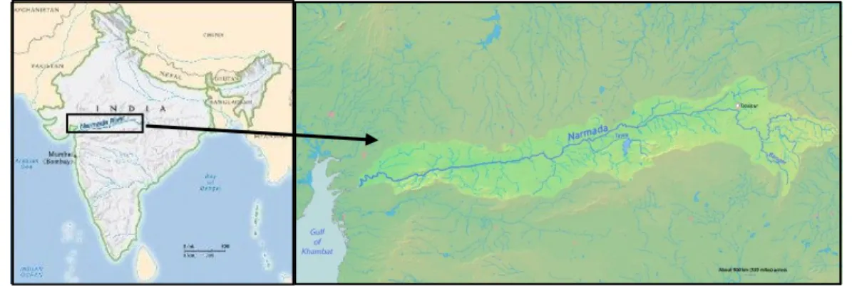
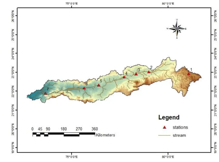
The Narmada River Basin stretches out over the states of Madhya Pradesh, Chhattisgarh, Maharashtra and Gujarat. This major river system heralds a territory of 98,796 square kilometres which is equivalent to 3 percent of the aggregate geographical expanse of the country. The maximum length of the river is 923 kilometres and its maximum width is 161 kilometers. It expands over 72°32’ E to 81°43’E longitudes and 21°27’N to 23°37’N latitudes. The Vindhya Ranges confine the river from the north, in the south it is limited by Satpura Ranges and the Maikala Ranges bound it from the north. The location of the river demarcates between the North and South India. This peninsular river flows towards the west, covering a distance of 1,312 kilometres and finally drains itself into the Arabian Sea via Gulf of Khambat, near the city of Bharuch at Gujarat. Figures 3.1 and 3.2 illustrate the location of River Narmada Basin and the various hydro-meteorological stations along River Narmada and its course with some of its tributaries.

15

Fig 3.2: Map showing the Stations selected for the analysis

3.1.1 The River Course and Physiography

The river originates from Maikala Range near the pilgrim town of Amarkantak in Annupur district, Madhya Pradesh with an elevation of approximately, 1057 metres. Along the mainstream, for the initial 1079 kilometres, it covers Madhya Pradesh. Later on, it constitutes a boundary between Maharashtra and Madhya Pradesh for 39 kilometers and Gujarat and Maharashtra for 35 kilometers. The state of Gujarat withholds 39 kilometers of the river. The different tributaries of the river system are the Banjar, the Burhner, the Shakkar, the Sher, the Dudhi, the Ganjal, the Tawa, the Goi, the Kundi and the Karjan. These tributaries connect with the river from the left.

16

The tributaries of Tendoni, Hiran, Kolar, Barna, Uri, Man, Orsang and Hatni connect with the river from the right.

The Narmada River Basin can be split up into plain and hilly areas. The hilly areas are covered with forests and cover the upper and lower middle expanses. The central area between the upper and lower reaches constitute of pain regions which are suitable for cultivation.

3.1.1.1Stations selected for the study

In the present study, seven stations have been chosen along the mainstream of the river. The sites are chosen according to the availability of data in a government portal. The different stations chosen are illustrated in the Table 3.1.

Table 3.1: Description of the Stations Studied

Sl. No. Name Location Resources/

Importance Population Distance Station 1 Dindori 22°50’44”N latitude 81°4’31.8”E longitude A hub of mineral resources like coal, bauxite, white ash, okars, high iron laterite and limestone 704,218 (according to 2011 census) 89.4 km from Amarkantak Station 2 Barmanghat 23°1’58.8”N latitude, 79°1’14.52”E longitude It is a holy place where River Warahi and Narmada unite. A fair is held each year during January. 7000 (according to 2008 census) Located 211.4 km from Station 1. Station 3 Sandhia 22°1’0.012”N latitude and 73°46’ 0.012” E longitude It is a medium sized village 767 (2011 census) Located 551.3 km away from Station 2. Station 4 Hoshangabad 22°44’38.76”N latitude, 77°44’13.2”E longitude A very significant station. Of religious importance. 117956 (2011) Located 416.1 km away from Station 3.

17 Ritual of mass bathing during mid-January. Station 5 Handia 25°21’41.76”N latitude, 82°11’21.48”E longitude This is a large village with many temples in the name of River Narmada 4221 (2011) Located 537.6 km away from Station 4. Station 6 Mandleshwar 22°10’36.84”N latitude, 75°39’36.36”E longitude It is an important town with a hydro-electric project near Maheshwar Dam. Agriculture is an important occupation here. 11345 (2001) Located 752.7 km away from Station 5. Station 7 Garudeshwar 21°53’32.64”N latitude and 73°39’7.56”E longitude An important holy place and a small village. 2452 (2011) Located 209.4 km away from Station 6.

3.1.2 The Climate and Rainfall

The overall climate of the river basin remains humid tropical. In the east it is sub-humid and in the west it is semi-arid. In the hilly areas, humid climate is prevalent.

The Tropic of Cancer divides the basin into a small northern zone and a large southern zone. The seasons of cold-weather (temperature 17.5 to 20°C), hot weather (temperature 30 to 32.5°C), south-west monsoon (temperature 27.5 to 30°C), and post-monsoon (temperature 25 to 27.5°C) are distinct in the basin.

The normal annual rainfall in the basin is 1178 centimetres with the predominant rainy season being the south-west monsoon from June to October. The upper hilly as well as plain expanses of the basin receive maximum rainfall.

18

3.1.3 Water Quality of mainstream Narmada River Basin

The percentage of utilization of surface water from River Narmada is 23 which is not very high as the river is inaccessible at most of the places. The river has attained global priority for conservation of aquatic biodiversity since 1988 by Jetkins and Groombridge. The water level has also degraded as per a report in 2014. More than fifty species of fishes have been made extinct because of the degrading water quality and anthropogenic activities.

According to the Water Quality Status Report of 2012, by Central Pollution Control Board, the desirable limits are being exceeded along the main stream of the river at Mandla, Hoshangabad, and Saraswati Ghat in Madhya Pradesh and at Bharuch and Panetha in the state of Gujarat. The lowest DO level measured at Narmada is 2.2 mg/L while the Coliform Count and Faecal Coliform count reach to 9000 and 7000 MPN/100mL respectively.

3.2 Data Collection and Analysis

Monthly water quality data are collected from relevant government sites from the year 1991 to 2013 for the seven chosen stations. Following are the twenty six parameters chosen for the analysis. The variation of each estimate for a typical year has been illustrated with the help of graphs.

3.2.1 Discharge (in cubic metres per second):

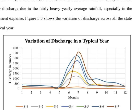
The water quality estimates measured in a river system account more for the river chemistry than the temporal dynamics. Distinct seasonal changes in such a system result in prominent variations in the river discharge. The concept of yearly loading of nutrients

19

into the river system depends on how the river chemistry transforms according to the temporal changes in discharge. Though River Narmada is rain fed, it gets a moderately heavy discharge due to the fairly heavy yearly average rainfall, especially in the upper catchment expanse. Figure 3.3 shows the variation of discharge across all the stations for a typical year.

Fig 3.3: Variation of Discharge for all the sites in a typical year

3.2.2 Temperature (in Degrees Celsius):

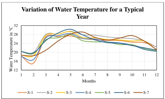
This is the most common physical water quality variable which affects the bio-chemical characteristics and the life system in water. The concentration of Dissolved Oxygen and various biological activities depend on what the temperature is. Figure 3.4 shows the variation of temperature across all the stations for a typical year.

0 500 1000 1500 2000 2500 3000 3500 4000 1 2 3 4 5 6 7 8 9 10 11 12 Dis ch ar g e in cu m ce s Months

Variation of Discharge in a Typical Year

20

Fig 3.4: Variation of Temperature for all the sites in a typical year

3.2.3 pH

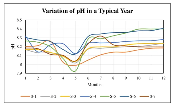
pH is another water quality estimate influenced by chemicals which in turn influences the acidity or the basicity of water. Bicarbonates of different metallic ions are responsible for alkalinity while mineral acids account for the acidity of water. Figure 3.5 shows the variation of pH across all the stations for a typical year.

12 16 20 24 28 32 1 2 3 4 5 6 7 8 9 10 11 12 W ater T em p er atu re in ° C Months

Variation of Water Temperature for a Typical

Year

21

Fig 3.5: Variation of pH for all the sites in a typical year

3.2.4 Electrical Conductivity in micro mho/cm

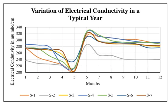
It is the measure of the capacity of water to allow electrical flow through it. Thus it accounts for the number of ions present in the water body. It is also an approximate estimate of Total Dissolved Solids. Metallic ions are responsible for an increase in Electrical Conductivity. Figure 3.6 shows the variation of discharge across all the stations for a typical year.

7.9 8 8.1 8.2 8.3 8.4 8.5 1 2 3 4 5 6 7 8 9 10 11 12 pH Months

Variation of pH in a Typical Year

22

Fig 3.6: Variation of Electrical Conductivity for all the sites in a typical year

3.2.5 Total Dissolved Solids in micro mho/cm

This parameter constitutes of all the ions, both organic and inorganic, which are less than 2 microns. Figure 3.7 shows the variation of Total Dissolved Solids across all the stations for a typical year.

Fig 3.7: Variation of Total Dissolved Solids for all the sites in a typical year

200 220 240 260 280 300 320 340 1 2 3 4 5 6 7 8 9 10 11 12 E lectr ical C o n d u tiv ity in m u m h o /cm Months

Variation of Electrical Conductivity in a

Typical Year

Variation of Total Dissolved Solids for a

Typical Year

23

3.2.6 Ammonia Ion Concentration in mg N /L:

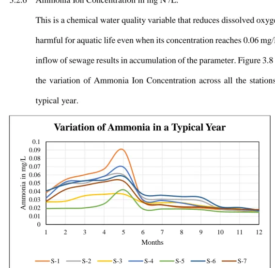
This is a chemical water quality variable that reduces dissolved oxygen and harmful for aquatic life even when its concentration reaches 0.06 mg/L. The inflow of sewage results in accumulation of the parameter. Figure 3.8 shows the variation of Ammonia Ion Concentration across all the stations for a typical year.

Fig 3.8: Variation of Ammonia Ion concentration for all the sites in a typical year

3.2.7 Nitrate and Nitrite Ions Concentration in mg N/L:

Nitrate ion concentration accounts for agricultural waste, waste water, human and animal wastes. Nitrite can be produced by Nitrosomonas Bacteria in stagnated water conditions with limited oxygen supply. Figure 3.9 shows the variation of Nitrate and Nitrite Ions Concentration across all the stations for a typical year.

0 0.01 0.02 0.03 0.04 0.05 0.06 0.07 0.08 0.09 0.1 1 2 3 4 5 6 7 8 9 10 11 12 A m m o n ia in m g /L Months

Variation of Ammonia in a Typical Year

24

Fig 3.9: Variation of Nitrate and Nitrite Ion concentration for all the sites in a typical year

3.2.8 Silicon Dioxide in mg/L:

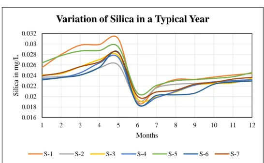
Disintegration of minerals and rocks account for the presence of silica in water. This estimate is an important growth component for microscopic plants like diatoms and also serve as a source of food for fishes. Though termed as corrosion inhibitors, if the concentration of silica exceeds certain limit, it makes the water unhealthy for consumption. Figure 3.10 shows the variation of Silicon Dioxide across all the stations for a typical year.

0 0.2 0.4 0.6 0.8 1 1.2 1.4 1.6 1.8 1 2 3 4 5 6 7 8 9 10 11 12 NO2 +N O3 in m g /L Months

Variation of Nitrate+Nitrite in a Typical Year

25

Fig 3.10: Variation of Silica concentration for all the sites in a typical year

3.2.9 Dissolved Oxygen in mg/L:

This is an important chemical parameter in water quality analysis. A certain amount of oxygen gets dissolved in a water body, is acclaimed as Dissolved Oxygen and accounts for the life within water. This parameter is sensitive to an increase in organic or inorganic pollution. Figure 3.11 shows the variation of Dissolved Oxygen across all the stations for a typical year.

Fig 3.11: Variation of Dissolved Oxygen concentration for all the sites in a typical year

0.016 0.018 0.02 0.022 0.024 0.026 0.028 0.03 0.032 1 2 3 4 5 6 7 8 9 10 11 12 Sil ica in m g /L Months

Variation of Silica in a Typical Year

S-1 S-2 S-3 S-4 S-5 S-6 S-7 2 3 4 5 6 7 8 9 10 11 1 2 3 4 5 6 7 8 9 10 11 12

Variation of Dissolved Oxygen in a Typical

Year

26

3.2.10 Biochemical Oxygen Demand in mg/L:

This parameter accounts for the amount of pollutants and organisms present in water. It is the quantity of DO consumed by microbes to catabolize organic matter in a water body. Hence an increase in BOD is harmful for the aquatic ecosystem. Figure 3.12 shows the variation of Biochemical Oxygen Demand across all the stations for a typical year.

Fig 3.12: Variation of Biochemical Oxygen Demand for all the sites in a typical year

3.2.11 Chemical Oxygen Demand in mg/L:

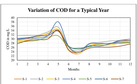
This chemical estimate accounts for the amount of oxidizable organics present in a water body due to discharge of wastewaters. An increase in COD decreases the amount of DO present and hence affects the aquatic life. Figure 3.13 shows the variation of Chemical Oxygen Demand across all the stations for a typical year.

0 0.5 1 1.5 2 2.5 3 3.5 1 2 3 4 5 6 7 8 9 10 11 12 B OD in m g /L Months

Variation of BOD for a Typical Year

27

Fig 3.13: Variation of Chemical Oxygen Demand for all the sites in a typical year

3.2.12 Phenol Ions Concentration in mg/L:

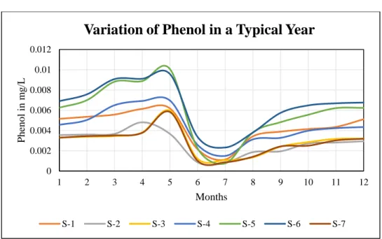
Initially employed as a disinfectant, this organic pollutant accounts for toxicity when available above its permissible limits. This variable enters into a water body because of incessant disposal of effluents from various industries. Figure 3.14 shows the variation of Phenol Ions Concentration across all the stations for a typical year.

20 22 24 26 28 30 32 34 36 38 40 1 2 3 4 5 6 7 8 9 10 11 12 C OD in m g /L Months

Variation of COD for a Typical Year

28

Fig 3.14: Variation of Phenol Ion Concentration for all the sites in a typical year

3.2.13 Total Alkalinity in mg CaCO3 /L:

This parameter accounts for the resistance of water body to change its pH and is identified by the concentration of carbonates, hydroxides and bicarbonates. Figure 3.15 shows the variation of Total Alkalinity across all the stations for a typical year.

Fig 3.15: Variation of Total Alkalinity for all the sites in a typical year

0 0.002 0.004 0.006 0.008 0.01 0.012 1 2 3 4 5 6 7 8 9 10 11 12 P h en o l in m g /L Months

Variation of Phenol in a Typical Year

S-1 S-2 S-3 S-4 S-5 S-6 S-7 100 120 140 160 180 200 220 1 2 3 4 5 6 7 8 9 10 11 12 T o tal A lk alin ity in m g C aCO 3 /L Months

Variation of Total Alkalinity in a Typical Year

29

3.2.14 Total Hardness in mg CaCO3 /L:

This estimate is reflected by the concentration of Calcium and Magnesium Ions present. Hard water is difficult to use and hence should be properly treated. Figure 3.16 shows the variation of Total Hardness across all the stations for a typical year.

Fig 3.16: Variation of Total Hardness for all the sites in a typical year

3.2.15 Calcium Hardness in mg CaCO3 /L:

This hardness accounts only for the calcium compounds. Figure 3.17 shows the variation of Calcium Hardness across all the stations for a typical year.

80 90 100 110 120 130 140 150 1 2 3 4 5 6 7 8 9 10 11 12 T o tal Har d n ess in m g C aCO3 /L Months

Variation of Total Hardness in a Typical Year

30

Fig 3.17: Variation of Calcium Hardness for all the sites in a typical year

3.2.16 Fluoride Ion Concentration in mg/L:

This variable when between 1.0 mg/L and 1.5 mg/L is good. If less than the permissible range, it causes tooth decay and if more causes skeletal and dental fluorosis. The main source of this pollutant are pesticides and pharmaceuticals. Figure 3.18 shows the variation of Fluoride Ions Concentration across all the stations for a typical year.

Fig 3.18: Variation of Fluoride Ion Concentration for all the sites in a typical year

55 60 65 70 75 80 85 90 1 2 3 4 5 6 7 8 9 10 11 12 C alciu m Har d n ess in m g C aCO 3 m g /L Months

Variation of Calcium Hardness in mg

CaCO

/L

Variation of Fluoride in a Typical Year

31

3.2.17 Calcium Major Ion Concentration in mg/L:

Originating from rocks like that of limestone and marble, this variable is a measure of the hardness of water. The maximum limit of calcium ions in drinking water is 50 mg/L. Figure 3.19 shows the variation of Calcium Major Ions Concentration across all the stations for a typical year.

Fig 3.19: Variation of Calcium Major Ion Concentration for all the sites in a typical year

3.2.18 Magnesium Ion Concentration in mg/L:

A ubiquitous ion in sea water, this parameter accounts for hardness along with Calcium. It occurs due to mineral resources, fertilizers and industrial wastes. Figure 3.20 shows the variation of Magnesium Ion Concentrations across all the stations for a typical year.

20 22 24 26 28 30 32 34 36 1 2 3 4 5 6 7 8 9 10 11 12 C alciu m Ma jo r Io n s in m g C aCO3 /L Months

Variation of Calcium Major Ions in a Typical

Year

32

Fig 3.20: Variation of Magnesium Ion Concentration for all the sites in a typical year

3.2.19 Sodium Ion Concentration in mg/L:

This is a very common estimate present in water. Saline intrusion, effluents from sewage and mineral deposits can result contribute to the presence of sodium ions in water. Figure 3.21 shows the variation of Sodium Ion Concentrations across all the stations for a typical year.

Fig 3.21: Variation of Sodium Ion Concentration for all the sites in a typical year

6 8 10 12 14 16 18 1 2 3 4 5 6 7 8 9 10 11 12 Ma g n esiu m I o n co n ce n tr atio n in m g /L Months

Variation of Magnesium Ions in a Typical Year

S-1 S-2 S-3 S-4 S-5 S-6 S-7 5 10 15 20 1 2 3 4 5 6 7 8 9 10 11 12 So d iu m I o n C o n ec n tr atio n in m g /L Months

Variation of Sodium Ion Concentration in a

Typical Year

33

3.2.20 Potassium Ion Concentration in mg/L:

An essential constituent in human body, this parameter is usually within its permissible limits in water. Weathering of minerals and leaching of fertilizers result in an increased concentration of potassium ions in water. Figure 3.22 shows the variation of Potassium Ion Concentration across all the stations for a typical year.

Fig 3.22: Variation of Potassium Ion Concentration for all the sites in a typical year

3.2.21 Chloride Ions Concentration in mg/L:

Leached from different rocks, chloride ions account for the salty taste to water when present above 250 mg/L. These ions may occur due to industrial and domestic wastes. Figure 3.23 shows the variation of Chloride Ions Concentration across all the stations for a typical year.

0.5 1 1.5 2 2.5 3 3.5 1 2 3 4 5 6 7 8 9 10 11 12 P o ttas iu m I o n C o n ce n tr atio n in m g /L Months

Variation of Potassium Ion Concentration in a

Typical Year

34

Fig 3.23: Variation of Chloride Ion Concentration for all the sites in a typical year

3.2.22 Sulphate Ions Concentration in mg/L:

This water quality variable originates from minerals like barite, epsomite and gypsum. The concentrations depend upon the cations associated with the sulphate ions. The wastewater from smelters and mines develop the concentration of this variable in water. Figure 3.24 shows the variation of Sulphate Ions Concentration across all the stations for a typical year.

Fig 3.24: Variation of Sulphate Ion Concentration for all the sites in a typical year

5 7 9 11 1 2 3 4 5 6 7 8 9 10 11 12 C h o rid e Io n C o n ce n tr atio n in m g /L Months

Variation of Chloride Ion Concentration in a

Typical Year

Variation of Sulphate Ion Concentration in a

Typical Year

35

3.2.23 Carbonate Ion Concentration in mg/L:

This estimate accounts for an increase in pH and alkalinity in a water sample. It is usually formed from the dissociation of carbon dioxide in water. Figure 3.25 shows the variation of Carbonate Ion Concentration across all the stations for a typical year.

Fig 3.25: Variation of Carbonate Ion Concentration for all the sites in a typical year

3.2.24 Bicarbonate Ion Concentration in mg/L:

Resulting from the attempt to balance the carbonate equilibria, this parameter is abundantly found in running waters. The erosion of limestone results in the formation of this anion. Figure 3.26 shows the variation of Bicarbonate Ion Concentration across all the stations for a typical year.

0 2 4 6 8 10 12 14 1 2 3 4 5 6 7 8 9 10 11 12 C ar b o n ate Io n C o n ce n tr atio n in m g /L Months

Variation of Carbonate Ion Concentration in a

Typical Year

36

Fig 3.26: Variation of Bicarbonate Ion Concentration for all the sites in a typical year

3.2.25 Total Coliform Count in MPN/100 mL:

This variable is the collection of different bacteria in water. This may not be harmful but has the potential of being victimized by pathogens. Severe environmental pollution is responsible for this estimate. Figure 3.27 shows the variation of Total Coliform Count across all the stations for a typical year.

Fig 3.27: Variation of Total Coliform for all the sites in a typical year

110 130 150 170 190 210 230 1 2 3 4 5 6 7 8 9 10 11 12 B icar b o n ate iOn C o n cen tratio n in m g /L Months

Variation of Bicarbonate Ion Concentration in

a Typical Year

Variation of Total Coliform in a Typical Year

37

3.2.26 Faecal Coliform Count in MPN/100 mL:

This variable results from anthropogenic pollution. The presence of pathogens is more prominent if a water sample contains Faecal Coliform. Figure 3.28 shows the variation of Faecal Coliform Count across all the stations for a typical year.

Fig 3.28: Variation of Faecal Coliform for all the sites in a typical year

0 2000 4000 6000 8000 10000 12000 14000 16000 18000 1 2 3 4 5 6 7 8 9 10 11 12 Faec al C o lif o rm C o u n t in MP N/ 1 0 0 m L Months

Variation of Faecal Coliform in a Typical Year

38

CHAPTER IV

METHDOLOGY

4.1 WATER QUALITY INDEX

Water quality indices can be devised by using increasing or decreasing scale indices. The method used in the current research work is of decreasing scale indices where the degree of pollution is inversely related to the index values. The formulation of water quality index involves four steps:

i) Selection of Parameters:

ii) Transformation of the selected parameters, having different units, into a common scale. iii) Assigning weights to the transformed parameters.

iv) Aggregating the results obtained in step (iii) to determine a final index value.

Out of the above given steps, all are mandatory except step (iii). Water Quality Indices facilitate common people to understand the level of pollution of any water resource. However, formulation of Water Quality Index is not that simple. Various subjective opinions and references from experts are necessary and complete objectivity cannot be attained. The steps mentioned are explained below:

4.1.1 Parameter Selection:

A Water Quality Index would become clumsy if all the constituents present in a water sample would be included in the process. Therefore one needs to select a set of variables which as a whole reflect the overall quality of water for any given use. This is the place where subjectivity pops out. Different experts may have different opinions regarding the choice of sensitive parameters.

39

In the current work, a method of Student’s t-test has been used to select three significant parameters from each chosen site.

4.1.1.1Student’s t-test:

Let us think of a small sample with size n from a normal population, having mean µ and standard deviation σ. Let ӯ be the mean and σs be the

standard deviation of the sample drawn. Then,‘t’ statistic is given by equation 4.1 as

𝑡 =

√𝑛

where n is the number of observations. When the‘t’ statistic of each sample is calculated, we get a t distribution which is essentially symmetric and is normally distributed for large samples. The t-test was found by W.S Gosset in 1908 under the pen name of Student and hence the name ‘Student’s t-test’. This hypothesis test tells us whether means of two samples are statistically significantly different from each other, the null hypothesis being the means are the same. Thus, t-test belongs to the category of inferential statistics. If the t value is big, then the two samples can be considered significantly different or vice versa. How big the t value should be is better determined using the p-value which is the probability of the t value of lying with the region of significance. There are two levels of significance i.e. 5% and 1%. If for a t-test p>0.05 (for 5% level of significance), the difference between ӯ and σ is not significant and if p<0.05 the means are significantly different. In the current study 5% significance level has been chosen. Considering monthly discharge as an

40

independent parameter, the t-test is conducted between each water quality variable and discharge. Thus from this hypothesis testing we identify the variables which are independent of discharge. Further a two-tailed test is adopted thus assuming the relationship possibility to be in both the directions. The concept of a t-distribution has been elaborated in Figure 4.1.

Fig 4.1: A typical two-sided t-distribution (PDF = probability density function)

4.1.2 Conversion of parameters of different units into a common scale:

Different parameters have different ranges of occurrence and different are measured in different units. pH has no unit and is limited to a value of 14. Dissolved Oxygen is measured in mg/L and is rarely beyond 12mg/L while sodium, being measured in the same unit may extend up to 1000mg/L. Toxic constituents like mercury occur mostly below 1mg/L. On the other hand, alkalinity and hardness always occur above 1mg/L. Still a water sample with a chloride content of 10mg/L is as healthy as one containing chloride fifteen times higher the former. But a water sample constituting of mercury of level 0.001mg/L is acceptable and one containing even twice of that is harmful.

41

Therefore transformation of the different parameters into a common scale is a necessity. The scale usually ranges from zero to one. It may also range from zero to hundred.

4.1.2.1 Development of Sub-indices:

Various mathematical functions are applied to formulate different pollutant variables, thus, generating sub-index functions. For n water quality variables x1, x2,

x3 and so on each variable is represented by a sub-index S.I.i calculated using a

function as per Equation 4.2:

𝑆. 𝐼.𝑖= 𝑓𝑖(𝑥𝑖)--- (4.2)

After computation of the sub-indices, they are aggregated to form a final value in the next mathematical step as shown in Equation 4.3.

𝐼 = 𝑔(𝑆. 𝐼1, 𝑆. 𝐼2,… 𝑆. 𝐼3) --- (4.3)

The function may be a summation or a multiplicative operation or some other aggregation method. The overall procedure for development of sub-indices has been explained in the Figure 4.2: