Multi-Objective Generation and Emission Dispatch Using NSGA-II

(1)

Abstract— The multi-objective problem of the generation and emission dispatch is solved to find the generation levels that best compromise the generation cost and the emission level while satisfying the power balance constraint. The solution is attempted using non-dominated sorting genetic algorithms–II (NSGA-II) to find non-dominated solutions of with good diversity. The best compromise solution has been obtained using Fuzzy cardinal priority ranking. The results are presented for a system of 6-generators by neglecting the losses and accounting them for different combinations of Fuel cost,

NOx, COx and SOx emission objectives. The simulated results demonstrate the effectiveness of the proposal formulation.

Index Terms— Generation dispatch, Emission dispatch, Multi-objective optimization, Evolutionary algorithm.

I. INTRODUCTION

The cost of power system operation is minimized by economic or generation dispatch, which is the allocation of generation to various units to meet a given load demand. For thermal units, operating cost is mainly due to the fuel cost. The operation of these units also produces large amount of emission like oxides of sodium SOX, nitrogen NOX, carbon

COX etc. These emissions, an environmental concern, have

forced the utilities to adopt various practices like use of higher quality fuel, upgrading older plants with new efficient cleaner plants or considering emission-free alternate forms of energy. The economic dispatch with reference to clean air act [2] has been discussed. The clean air act persuades the utilities to change their practices to meet the environmental emission norms. Thus, it becomes important to perform the emission dispatch with generation dispatch.

Many studies have been carried out to solve the generation dispatch with or without emission dispatch. These studies include use of Goal programming techniques [3], Linear programming techniques [4], fuzzy approach [5,6] and Evolutionary Algorithms [7-11].

The generation and emission dispatch problem has been reduced to a single objective problem [12,13] by treating the emission as a constraint with a permissible limit. Alternatively, minimizing the emission has been handled as another objective in addition to usual cost objective. A linear programming based optimization by considering one objective at a time has been presented in [14]. The multi-objective emission and generation dispatch problem

Manuscript received April 26, 2011; revised August 31, 2011.

Javed Dhillon is with Alternate Hydro Energy Center, Indian Institute of Technology, Roorkee, Uttarakhand, India. (e-mail: [email protected])

Sanjay K. Jain is with Electrical and Instrumentation Engineering Department, Thapar University, Patiala, India. (e-mail: [email protected])

has been converted to a single objective problem by linear combination of different objectives as a weighted sum [15,16]. A set of non-inferior (or Pareto-optimal) solutions is obtained by varying the weight and therefore requires multiple runs. Goal programming method was also proposed for multi-objective generation and emission dispatch problem [17]. This method requires a prior knowledge about the shape of the problem search space.

The methods arising from evolutionary computation are fast and effective techniques capable of finding a well-distributed set of diverse trade-off solutions, with little or no more effort than sophisticated single-objective optimizer. Most multi-objective evolutionary algorithms (MOEAs) use the concept of Pareto domination to guide the search. A solution is said to dominate another solution, if it is no worse than other in all objectives and better than in at least one objective. A solution is said to be non dominated if it is not dominated by any other solution. Various evolutionary algorithms in [18, 19] are reported for multi-objective optimization.

In this paper, an elitist evolutionary non-dominated sorting algorithm (NSGA-II) is used for solving the multi-objective generation and emission dispatch problem. After obtaining various optimal solutions using NSGA-II, the single best compromise solution is obtained using Fuzzy cardinal priority ranking.

II.MULTI-OBJECTIVE GENERATION AND EMISSION DISPATCH

Multi-objective problems are often characterized by several non commensurable and often competing objectives [6, 7] subjected to a number of equality and inequality constraints. The general structure of multi-objective generation and emission dispatch problem is expressed as- Find : [PG] =[PG1, PG2, ….PGNg]T

By Minimizing: F = [FFC, FNX, FCX, FSX]

Subjected to: h(PGi) = 0

g(PGi) ≤ 0 (1)

where, i = 1, 2, 3……Ng

where Ng is the total no of generation units, PGiis the real

power output of ith generator, h(PGi) is the equality

constraints and g(PGi) is the inequality constraints.

The various objective functions for the generation and emission dispatch problem are :

A. Minimization of Fuel Cost (FFC) B. Minimization of NOX Emission (FNX) C.Minimization of COX Emission (FCX) D.Minimization of SOX Emission (FSX)

Multi-Objective Generation and Emission Dispatch Using

NSGA-II

(2)

A. Minimization of Fuel Cost (FFC)

The minimization of total fuel cost FFC is expressed as,

(

2

)

1 min

Ng

FC i i Gi i Gi

i

F a b P c P

=

∑

+ + $/hr (2)

whereai, biand ci are the fuel cost coefficient

B. Minimization of NOX emission (FNX)

The minimization of NOX emission FNX is represented as,

(

2

)

1 min Ng

NX Ni Ni Gi Ni Gi

i

F a b P c P

=

∑

+ + kg/hr (3)

whereaNi, bNiand cNi are the NOX emission coefficient

C. Minimization of COX emission (FCX)

The minimization of COXemission FCX is expressed as,

(

2

)

1 min

Ng

CX Ci Ci Gi Ci Gi

i

F a b P c P

=

∑

+ + kg/hr (4)

wherea_Ci, b_Ciand c_Ci are the COX emission coefficient

D. Minimization of SOX emission (FSX)

The minimization of SOX emission FSX is represented as,

(

2

)

1 min Ng

SX Si Si Gi Si Gi

i

F a b P c P

=

∑

+ + kg/hr (5)

whereaSi, bSiand cSi are the SOX emission coefficient

Power balance constraints

The total power generation must be equal to the total demand PD and the real transmission loss PLOSS. Hence,

( ) 0

1

= − −

∑

=

LOSS D Ng

i

Gi P P

P (6)

Where PLOSS is the total power loss given as below

∑ ∑

= =

=

Ng

i Ng

j

Gj ij Gi LOSS P B P

P

1 1

(7)

Limits on generator output PGi

For stable operation, the generator outputs must be within the limiting values as follows:

max min Gi Gi Gi P P

P ≤ ≤ (8)

III. ELITIST MULTI-OBJECTIVE EVOLUTIONARY ALGORITHM

The main objective of multi-objective evolutionary algorithm is to find multiple Pareto-optimal solutions in one single simulation run [8]. To enhance the convergence properties of multi-objective elitist operator [9] is used. The elitism helps to keep the best solution of the current population and does not allow it to deteriorate in next generation.

The NSGA-II which is known as elitist non-dominated sorting genetic algorithm, has the following features: 1) It uses non dominated sorting techniques to provide the

solution as close as possible to the pareto-optimal solution.

2) It uses crowding distance techniques to provide diversity in solution.

3) It uses elitist techniques to preserve the best solution of current population in next generation.

There are two stages in solving multi-objective problem: determination of the set of non-dominated solutions and selection of the best compromise solution.

A. Description of Algorithm based on NSGA-II

1) Initialize the population Pt.

2) Create the offspring population Qt from the current

population Pt.

3) Combine the two populations Qt and Pt to form Rt

where Rt = Pt U Qt

4) Find non-dominated fronts Fiof Rt.

5) Initiate the new population Pt+1 = null and the counter

of front for inclusion i = 1.

6) While Pt+1 + Fi ≤ Npop, do: Pt+1←Pt+1 U Fi, where i ←

i+1

7) Sort the last front Fi using the crowding distance in

descending order and choose the first (Npop – Pt+1)

elements of Fi

8) Use selection, crossover and mutation operators to create the new offspring population Qt+1 .

Initialization

Initialize the population Pt by the randomly generating

PGi’s and satisfying power balance equation (6). After

initialization it creates offspring population Qt from the

current population Pt and then combines the two populations

to form Rt. Where Rt is define as:

Rt = Pt U Qt

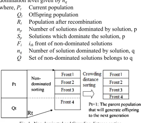
Non-Dominated Sorting

After the initialization the population is sorted on the basis of on non-domination as shown in Fig. 1. The pseudo code for this is -

for each (p∈P) for each (q∈P) if (ppq)then

Sp =Sp∪_{{ }}q

elseif (qp p)then np =np+1 end

end

if (np ==0)then F1=F1∪_{{ }}p

end end

The pseudo code suggests that if p dominates q then add q

in the set Sp. If p dominated by q then increment the

dominated counter np by 1. If there is no any solution which

dominate p i.e (np = 0), then p belong to first front F1.

while (Fi ≠null) Q=null

(3)

If (nq =0) then Q=Q∪_{{ }}q

end end end

i = i+1

Fi =Q

end

Assign the front to each q in the set Sp according to its

domination level given by nq

where, Pt Current population

Qt Offspring population

Rt Population after recombination

np Number of solutions dominated by solution, p

Sp Solutions which dominate the solution, p

Fi ith front of non-dominated solutions

nq Number of solution dominated by solution, q

Q Set of non-dominated solutions belongs to q

Fig. 1. Non-dominated and Crowding distance sorting

Crowding distance

To provide the diversity in population, the crowding distance is calculated[19]. The following pseudo code is used to calculate the crowding distance of each point in set I.

l = |I|

for each i

set I[i]distance = 0

end for each m

I = sort(I,m)

I[1]distance = I[l]distance = ∞

end

for (I = 2 to ( l - 1) )

I[i]distance = I[i]distance +

) /(

) ). 1 ( ). 1 (

( max min

m m f

f m k I m k

I + − − −

end

Firstly assign the boundary value to infinity and then calculate the crowding distance. Here, I(k).m is the crowding distance for the mth objective function of the kth individual.

Where, I Set of non-dominated solutions

l Total number of solutions in set I m Number of objective functions

fmmax Maximum fitness value of mth objective function

fmmin Minimum fitness value of mth objective function

Selection

Once the individuals are sorted based on non-domination with the crowding distance assigned, the selection is carried out using a crowded-comparison-operator (>n) and best solution is selected. As shown in Fig. 1, it will be used to

create Front 4 of small size than obtained after the non-dominated sorting. It assumes that every solution has two attributes:

1) A Non-domination rank (ri) in population

2) A local Crowding distance (I[i]distance)

i >n j

if (ri < rj)

or

if ((ri = rj) and (I[i]distance > I[j]distance))

The solution i is better than j if rank of ith solution is better

than jth or if they have same rank but the crowding distance of

ith solution is better than jth

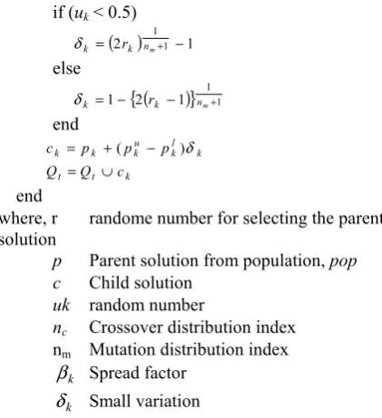
Crossover and Mutation

The real coded genetic algorithm [10] employed in this paper uses Simulated Binary Crossover and Polynomial Mutation to create population Qt as shown in Fig. 2 .

Fig. 2. Crossover and Mutation operation

1) Simulated Binary Crossover (SBX)

To generate the offsprings or child solutions using crossover, randomly select two parents solution (p1,k, p2,k) from the initial population and then generate the two child solution (c1,k, c2,k) as per the given pseudo code.

Npop = |pop|

for each k

r1,k = random(1,Npop)

r2,k = random(1,Npop)

p1,k = pop(r1,k)

p2,k = pop(r2,k)

uk= random(0,1)

if (uk > 0.5) ( )₂ 1/( +1)

= nc

k k u

β

else

( )

{ }1/( 1) 1 2

1

+

− =

c n k k

u β

end

c1.k = ½ [(1-βk).p1,k + (1+βk).p2,k]

c2.k = ½ [(1+βk).p1,k + (1-βk).p2,k]

Qt = Qt U c1.k

Qt = Qt U c2.k

end

2) Polynomial Mutation

This operator randomly selects one parent solution from the population and applies the mutation operator to generate a single offspring. The pseudo code is given as :

for each k

rk = random(1,Npop)

pk = pop(rk)

(4)

if (uk < 0.5)

( )2 1 1

1

− = k nm+ k r

δ

else

_{ ₍ ₎_} 1 1 1 2

1− − +

= k nm

k r

δ

end

l _k

k u k k

k p p p

c = +( − )δ

Q_t =Q_t ∪c_k

end

where, r randome number for selecting the parent solution

p Parent solution from population, pop c Child solution

uk random number

nc Crossover distribution index

nm Mutation distribution index k

β Spread factor k

δ Small variation

B. Best Compromise Solution

The optimization of the above-formulated multi-objective formulation using NSGA-II yields set of Pareto optimal solutions [11], in which one objective cannot be improved without sacrificing other objectives. For practical applications, however, we need to select one solution, which will satisfy the different goals to some extent. Such a solution is called best compromise solution. The best compromise solution is obtained using Fuzzy cardinal priority ranking. The pseudo code for this is given as:

for each (k∈M) for each (i∈Nobj) if(fik ≥ fmaxM ) k =0

i

u

else if (fminM ≤ fik ≤ fmaxM )

(

k

) (

M M

)

i M k

i f f f f

u = max − / max − min

else k =1

i

u

end end end

for each (i∈Nobj)

⎟ ⎟ ⎠ ⎞ ⎜

⎜ ⎝ ⎛

=

∑

∑ ∑

= =

=

obj N

i M

k k i M

k k i

i u u

1 1 1

/

β

end

where _β_i is the normalize membership function. The

i

β provides the fuzzy cardinal priority ranking of the non-dominated solution. the solution that attains the maximum membership β_iin fuzzy set is considered as best compromise solution.

where, Nobj Number of non-dominated solutions

k i

u Membership for kth objective and ith solution i

β Cardinal pirority ranking

IV. RESULTS AND DISCUSSION

The study is carried out for a system of six generators [20] detailed in the Appendix. The results are obtained for multi-objective generation and emission dispatch by using the power balance and generator capacity constraints for the following five cases of optimization formulations:

Case-A Fuel Cost and NOX Emission Case-B Fuel Cost and COX Emission Case-C Fuel Cost and SOX Emission

Case-D Fuel Cost, NOX Emission and COX Emission Case-E Fuel Cost, NOX Emission and SOX Emission

The results are obtained by neglecting and considering the losses at the load demand of 1800 MW with the following parameters -

• Population size = 100

• Maximum generation = 20000

• Crossover Distribution index = 20

• Mutation Distribution index = 20

• Crossover Probability = 0.9

• Mutation Probability = 0.1

In typical NSGA-II implementations, the mutation rate is small, typically around 10%. Whereas crossover rate is high, typically around 90%. The proposed study is carried out for two and three objectives functions to yield the relationship between the thermal units operating costs and emission. In all the cases the size of the initial population is 100. The maximum generations are 6000 and 20000 for the optimization of two and three objectives respectively.

A. Multi-Objective optimization when losses are neglected

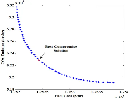
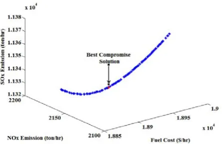
The results obtained for the multi-objective optimization using the developed algorithm for the above mentioned Cases are summarized in Table I-V. The Table summarizes the solution at the minimum of the respective objective function and the best compromise solution for the respective set of objectives considered. In Case A, B and C two objectives are considered, the pareto optimal front for these are having similar nature. As a sample case the Pareto optimal fronts for case-B, case-D and case-E are shown in Fig. 3, Fig. 4 and Fig. 5 respectively. From the Tables I-V, it is clear that the minimum fuel cost is obtained close to 17520. The marginal difference is due to the solution is being run at different occasion and the convergence is based on evolutionary technique. The cost corresponding to best compromise solution is bound to change as it depends on all the objectives under investigation. The cost in best compromise solution is changing between 17520-17530.

B. Multi-Objective Optimization by Accounting Losses

(5)

respectively. The total fuel cost for the best compromise solution changes marginally around Rs. 18900.

TABLEI:RESULT FOR FUEL COST AND NOXOPTIMIZATION

TABLEII:RESULT FOR FUEL COST AND COX OPTIMIZATION

Units (in MW)

Solution at minimum FFC

Solution at minimum FCX

Best Compromise Solution

PG1 221.8656 250.0000 238.9509 PG2 229.9998 229.9999 229.9994 PG3 437.0433 402.1071 419.3458 PG4 264.9987 264.9987 264.9961 PG5 441.7217 405.8301 424.0666 PG6 202.5707 245.2628 220.84114 FFC ($/hr) 17520.2842 17537.8799 17524.0739

FCX (kg/hr) 53260.5444 51912.1721 52308.2522

TABLEIII:RESULT FOR FUEL COST AND SOXOPTIMIZATION

Units (in MW)

Solution at minimum FSX

FSX (kg/hr) 10510.5739 10510.2146 10510.2916

TABLEIV:RESULT FOR FUEL COST,NOXAND COXOPTIMIZATION

Units (in MW)

Solution at minimum

FFC

Solution at minimum

FNX

Solution at minimum

FCX

Best Compromise

Solution

PG1 222.3661 166.8411 250.0000 197.9152

PG2 230.0000 194.2191 229.9987 229.7943

PG3 438.5525 486.0322 404.5769 454.4389

PG4 264.9977 264.9365 264.9993 264.9926

PG5 438.8981 486.1711 403.4438 448.8072

PG6 203.3856 200.0000 245.1813 202.2704

FFC ($/hr) 17520.2987 17582.2152 17537.8536 17522.6806 FNX(kg/hr) 1848.9139 1805.3370 1929.2176 1828.2927 FCX(kg/hr) 53212.0024 58053.8654 51911.6072 54114.1258

TABLEV:RESULT FOR FUEL COST,NOXAND SOXOPTIMIZATION

Units (in MW)

Solution at minimum

FFC

Solution at minimum

FNX

Solution at minimum

FSX

Best Compromise

Solution

PG1 222.9468 166.4123 209.1126 173.5119

PG2 229.9999 194.1320 229.9999 229.6355

PG3 438.1437 486.0273 446.8517 465.7849

PG4 264.9942 264.9999 264.9982 264.9944

PG5 442.1101 486.6284 447.0476 464.2745

PG6 200.0000 200.0000 200.1898 200.0000

FFC ($/hr) 17520.3408 17582.5052 17520.9603 17528.5431 FNX(kg/hr) 1847.2415 1805.3021 1834.9453 1816.6648

FSX(kg/hr) 10510.6022 10544.2067 10510.2455 10512.8993

Fig. 3. Pareto optimal solution for fuel cost and COX optimization

Fig. 4. Pareto optimal solution for fuel cost NOX and COX optimization

Fig. 5. Pareto optimal solution for fuel cost NOX and SOX optimization

Fig. 6. Pareto optimal solution for fuel cost and NOX optimization Units

(in MW)

Solution at minimum FNX

(6)

TABLEVI:RESULT FOR FUEL COST AND NOXOPTIMIZATION

Units (in MW)

FNX (kg/hr) 2175.0972 2116.9552 2136.9552

TABLEVII:RESULT FOR FUEL COST AND COXOPTIMIZATION

Units (in MW)

FCX (kg/hr) 64013.6629 63931.8286 63952.1125

TABLEVIII:RESULT FOR FUEL COST AND SOXOPTIMIZATION

Units (in MW)

Solution at minimum FSX

FSX (kg/hr) 11326.0965 11326.0965 11326.0965

TABLEIX:RESULT FOR FUEL COST,NOXAND COXOPTIMIZATION

Units (in MW)

Solution at minimum

FFC

Solution at minimum

FNX

Best Compromise

Solution

PG1 250.0000 229.6664 250.0000 249.4301

PG2 229.9998 229.9634 229.9972 229.9874

PG3 499.9998 500.0000 499.9999 499.9865

PG4 265.0000 264.9983 264.9999 264.9866

PG5 417.1908 500.0000 430.1076 456.5024

PG6 276.9186 226.1944 265.3245 242.7227

FFC ($/hr) 18879.9055 18964.7177 18881.8366 18898.0244 FNX(kg/hr) 2180.4788 2116.9621 2163.3075 2137.8856 FCX(kg/hr) 64016.0833 65823.4113 63931.7113 64243.3887

TABLEX:RESULT FOR FUEL COST,NOXAND SOXOPTIMIZATION

Units (in MW)

Solution at minimum

FFC

Solution at minimum

FSX

Best Compromis

e Solution

PG1 250.0000 230.2076 250.0000 249.4956

PG2 229.9866 229.9999 229.9866 229.9999

PG3 500.0000 500.0000 500.0000 499.9452

PG4 264.9986 264.9999 264.9986 264.9983

PG5 421.7120 500.0000 421.7121 460.1639

PG6 272.8569 225.5907 272.8567 239.4992

FFC ($/hr) 18880.1700 18964.2999 18880.1700 18901.3563 FNX(kg/hr) 2174.1202 2116.9615 2174.1202 2135.3562

FSX(kg/hr) 11326.1342 11374.9355 11326.1342 11338.3420

Fig. 7. Pareto optimal solution for fuel cost, NOX and COX optimization

Fig. 8. Pareto optimal solution for fuel cost, NOX and SOX optimization

V.CONCLUSION

The multi-objective Generation and emission dispatch problem has been solved using the elitist Non-dominated Sorting Genetic Algorithm. The algorithm has been run on the six generator system by considering the system with or without loss. The study has been extended to two and three objectives problems. The following conclusions are made

• The developed algorithm provides pareto optimal solution with good diversity and best compromise solution.

• In the minimum fuel cost for neglecting the losses (or consider the losses) for different cases is same whereas the cost for best compromise solution in different because it depends on all the objectives considered, however the variation is small.

APPENDIX

The fuel cost, emission and loss coefficients for six generator system are given in Table A1, A2, A3, A4 and A5 respectively.

TABLEA1:FUEL COST COEFFICIENTS

Units _c_i _b_i _a_i _P_min _P_max

1 0.002035 8.43205 85.6348 100 250

2 0.003866 6.41031 303.7780 50 230

3 0.002182 7.42890 847.1484 200 500

4 0.001345 8.31540 274.2241 85 265

5 0.002162 7.42289 847.1484 200 500

(7)

TABLEA2:NOXEMISSION COEFFICIENTS

Units _c_Ni _b_Ni _a_Ni

1 0.006323 -0.38128 80.9019

2 0.006483 -0.79027 28.8249

3 0.003174 -1.36061 324.1775

4 0.006732 -2.39928 610.2535

5 0.003174 -1.36061 324.1775

6 0.006181 -0.39077 50.3808

TABLEA3:COXEMISSION COEFFICIENTS

Units _c_Ci _b_Ci _a_Ci

1 0.265110 -61.01945 5080.148 2 0.140053 -29.95221 3824.770 3 0.105929 -9.552794 1342.851 4 0.106409 -12.73642 1819.625 5 0.105929 -9.552794 1342.851 6 0.403144 -121.9812 11381.070

TABLEA4:SOXEMISSION COEFFICIENTS

Units _c_Si _b_Si _a_Si

1 0.001206 5.09928 51.3778

2 0.002320 3.84654 182.2605

3 0.001284 4.45647 508.5207

4 0.000813 4.97641 165.3433

5 0.001284 4.45647 508.5207

6 0.003578 4.14938 121.2133

TABLEA5:B-COEFFICIENTS

2.0e-4 1.0e-5 1.5e-5 5.0e-6 0.0 -3.0e-5 1.0e-5 3.0e-4 -2.0e-5 1.0e-6 1.2e-5 1.0e-5 1.5e-5 -2.0e-5 1.0e-4 -1.0e-5 1.0e-5 8.0e-6 5.0e-6 1.0e-6 -1.0e-5 1.5e-4 6.0e-6 5.0e-5 0.0 1.2e-5 1.0e-5 6.0e-6 2.5e-4 2.0e-5 -3.0e-5 1.0e-5 8.0e-6 5.0e-5 2.0e-5 2.1e-4

REFERENCES

[1] D. P. Kothari and I. J. Nagrath, Modern Power System Analysis, 3rd_ed., Tata McGraw-Hill, 2003.

[2] A. A. El-Keib, H. Ma and J. L. Hart, “Economic dispatch in view of the clean air act of 1990,” IEEE Trans. on Power Systems., vol. 9, no. 2, pp. 972–978, 1994.

[3] J. Nanda, D. P. Kothari and K. S. Lingamurthy, "Economic Emission Load Dispatch throughGoal Programming Technique," IEEE Trans. on Energy Conversion, vol. 3, no. 1, pp. 26-32, 1988.

[4] A. Farag, S. A1-Baiyat and T. C. Cheng, “Economic Load Dispatch Multiobjective optimization Procedures Using Linear Programming Techniques,” IEEE Trans. on Power Systems, vol. 10, no. 2, pp. 731-738, 1995.

[5] D. Srinivasan, C. S. Chang, and A. C. Liew, “Multiobjective Generation Schedule using Fuzzy Optimal Search Technique,” IEE Proceedings on Generation, Transmission & Distribution., vol. 141, no. 3, pp. 231-241, 1994.

[6] C. M. Huang, H. T. Yang and C. L. Huang, “Bi-Objective Power Dispatch Using Fuzzy Satisfaction- Maximizing Decision Approach,”

IEEE Trans. on Power Systems, vol. 12, no. 4, pp. 1715-1721, 1997. [7] M. A. Abido, “Multiobjective Evolutionary Algorithms for Electric

Power dispatch Problem,” IEEE Trans. on Evolutionary Computation, vol. 10, no. 3, pp. 315-329, 2006.

[8] K. Deb, A. Pratap, S. Agarwal and T. Meyarivan, “A Fast Elitist Multi-objective Genetic Algorithm: NSGA-II,” IEEE Trans. on Evolutionary Computation, vol. 6, no. 2, pp. 182 -197, 2002.

[9] E. Zitzler, K. Deb and L. Thiele, “Comparison of multiobjective evolutionary algorithms: Empirical results,” IEEE Trans. on Evolutionary Computation, vol. 8, no. 2, pp. 173-195, 2000.

[10] H. G. Beyer and K. Deb, “On Self-Adaptive Features in Real-Parameter Evolutionary Algorithm,” IEEE Trans. on Evolutionary Computation, vol. 5, no. 3, pp. 250- 270, 2001.

[11] R. T. F. Ah King and H. C. S. Rughooputh, “Elitist Multiobjective Evolutionary Algorithm for Environmental/Economic Dispatch”, IEEE Congress on Evolutionary Computation, Canberra, Australia, vol. 2, pp. 1108-1114, 2003.

[12] S. F. Brodesky and R. W. Hahn, “Assessing the Influence of Power Pools on Emission Constrained Economic Dispatch,” IEEE Trans. on Power Systems, vol. 1, no. 1, pp. 57-62, 1986.

[13] G. P. Granelli, M. Montagna, G. L. Pasini and P. Marannino, “Emission Constrained Dynamic Dispatch,” Electric Power Systems Research, vol. 24, pp. 56-64, 1992.

[14] A. Farag, S. Al-Baiyat and T. C. Cheng, “Economic Load Dispatch Multiobjective optimization Procedures Using Linear Programming Techniques,” IEEE Trans. on Power Systems, vol. 10, no. 2, pp. 731-738, 1995.

[15] J. Zahavi and L. Eisenberg, “Economic-Environmental Power Dispatch,” IEEE Trans. on Power Systems, Man and Cybernetics, vol. 5, no. 5, pp. 485-489, 1985.

[16] C. S. Chang, K. P. Wong and B. Fan, “Security-Constrained Multiobjective Generation Dispatch Using Bicriterion Global Optimization,” IEE Proceedings on Generation, Transmission & Distribution, vol. 142, no. 4, pp. 406-414, 1995.

[17] J. Nanda, D. P. Kothari and K. S. Lingamurthy, "Economic Emission Load Dispatch throughGoal Programming Technique," IEEE Trans. on Energy Conversion, vol. 3, pp. 26-32, 1988.

[18] E. Zitzler and L. Thiele, “Multiobjective evolutionary algorithms: A comparative case study and the strength pareto approach,” IEEE Trans. Evolutionary Computation, vol. 3, pp. 257–271, 1999.

[19] K. Deb, “Multiobjective Optimization using Evolutionary Algorithms,” Wiley-Interscience Series in Systems and Optimization, John Wiley & Sons, 2001.

[20] J. S. Dhillon and D. P. Kothari, “The surrogate worth trade-off approach for multiobjective thermal power dispatch problem,” Electric. Power Systems Research, vol. 56, no. 2, pp. 103-110, 2000.

Javed Dhillon, born in 1986 had his graduation from RIMT-IET, Mandigobindgarh, Punjab, India in 2007. He did ME in Power Systems & Electric Drives from Electrical & Instrumentation Engineering Department, Thapar University, Patiala, India in 2009. He is presently pursuing the Phd from Indian Institute of Technology, Roorkee, India. The research interest includes Optimal Power Flow, Application of Genetic Algorithms for Power System Operation.

Sanjay K. Jain, born in 1971 had his graduation from