A Study on Deep Learning: Training, Models and Applications

(1)

A STUDY ON DEEP LEARNING: TRAINING,

MODELS AND APPLICATIONS

HENGYUE PAN

A DISSERTATION SUBMITTED TO THE FACULTY OF GRADUATE STUDIES

IN PARTIAL FULFILLMENT OF THE REQUIREMENTS FOR THE DEGREE OF

DOCTOR OF PHILOSOPHY

GRADUATE PROGRAM IN

ELECTRICAL ENGINEERING AND COMPUTER SCIENCE YORK UNIVERSITY

TORONTO, ONTARIO April 2017

c

(2)

Abstract

In the past few years, deep learning has become a very important research field that has attracted a lot of research interests, attributing to the development of the computational hardware like high performance GPUs, training deep models, such as fully-connected deep neural networks (DNNs) and convolutional neural networks (CNNs), from scratch becomes practical, and using well-trained deep models to deal with real-world large scale problems also becomes possible. This dissertation mainly focuses on three im-portant problems in deep learning, i.e., training algorithm, computational models and applications, and provides several methods to improve the performances of different deep learning methods.

The first method of this dissertation is a DNN training algorithm called Annealed Gra-dient Descent (AGD). During the DNN optimization procedure, AGD optimizes a se-quence of gradually improved smoother mosaic functions that approximate the origi-nal non-convex objective function according to a pre-defined annealing schedule. This dissertation presents a theoretical analysis on the convergence properties and learning speed of AGD to show its benefits. The proposed AGD algorithm is applied to learn DNNs for hand-written digital recognition in MNIST database and speech recognition in Switchboard database. Experimental results have shown that AGD yields comparable performance as SGD but it can significantly expedite training of DNNs in big data sets (by about 40% faster).

Secondly, this dissertation proposes to apply a novel model, namely Hybrid Orthogonal Projection and Estimation (HOPE), to CNNs to introduce orthogonality into the net-work structure. HOPE can be viewed as a hybrid model to combine feature extraction with mixture models. It is an effective model to extract useful information from the original high-dimension feature vectors and meanwhile filter out irrelevant noises. In this work, three different ways to apply the HOPE models to CNNs, i.e.,HOPE-Input, single-HOPE-Blockandmulti-HOPE-Blocks, are presented. ForHOPE-InputCNNs, a

(3)

HOPE layer is directly used right after the network input to de-correlate high-dimension input feature vectors. Alternatively, insingle-HOPE-Blockandmulti-HOPE-Blocks C-NNs, the HOPE layers are used to replace one or more blocks in the CC-NNs, where one block may include several convolutional layers and one pooling layer. The experimental results on CIFAR-10, CIFAR-100 and ImageNet databases have shown that the orthogo-nal constraints imposed by the HOPE layers can significantly improve the performance of CNNs in the image classification tasks. In the CIFAR experiments, HOPE CNNs achieve one of the best performance when image augmentation has not been applied, and top 5 performance with image augmentation.

The third proposed method is to apply CNNs to a task called image saliency detec-tion, and achieves good performance. In this approach, a gradient descent method is used to iteratively modify the input images based on pixel-wise gradients to reduce a pre-defined cost function, which is defined to measure the class-specific objectness and clamp the class-irrelevant outputs. This designation can help to maintain image back-ground when modify the images. The pixel-wise gradients can be efficiently computed using the back-propagation algorithm. Moreover, SLIC superpixels and LAB color based low level saliency features are applied to smooth and refine the saliency maps. The CNNs based saliency method is quite computationally efficient, much faster than other state-of-the-art deep learning based saliency methods. Experimental results on two benchmark tasks, namely Pascal VOC 2012 and MSRA10k, have shown that the proposed methods can generate high-quality salience maps, at least comparable with many slow and complicated deep learning methods.

The last method is also for image saliency detection tasks. However, this method is based on a class of deep learning model called Generative Adversarial Network (GAN). The proposed method follows the basic idea of GAN, i.e., training two models simul-taneously: the G-Network takes images as inputs and can generate corresponding syn-thetic saliency maps, and the D-Network can determine if the sample is a synsyn-thetic saliency map rather than ground-truth saliency map. However, different from GAN, the proposed method uses fully supervised learning to learn both G-Network and D-Network. Therefore, the proposed method is called Supervised Adversarial Network (SAN). Moreover, SAN introduces a different G-Network and conv-comparison layers to further improve the saliency performance. Experimental results show that the SAN model can also generate state-of-the-art saliency maps for complicate images.

(4)

Acknowledgments

First and foremost, I would like to express my highest appreciation to my supervisor Professor Hui Jiang for his kind and continuous support to my study and research. He tells me how to find good ideas in the related research field and implement them, and al-so gives me enough freedom to work by myself. By discussing with him, I can gradually improve my idea and achieve better results.

I am also thankful to Professor Shiyao Jin in National University of Defense Technology (NUDT) in China. He is the supervisor of my graduate study from 2010 to 2012. He helped me to make change from a undergraduate student to a graduate student. I learned that courses study is not all for graduate students. Instead, we need to do research, read papers and try to publish our own research results. By working in his research group, I began to learn the basic ideas of computer vision and read a lot of related papers, which are important for my further research in York University.

I hope to express gratitude to my co-supervisors Professor Aijun An and Professor James Elder. They also provide me with a lot of help through the daily discussion and annual meetings. With their help, I passed the qualifying examination and thesis proposal, and work well on my research.

I would like to express gratitude to China Scholarship Council (CSC), which provides me with scholarship to support my Ph.D. study in York University. The scholarship helps me a lot and make me do not need to worry about money matters.

I would like to express appreciation to York University and the department of electrical engineering and computer science (EECS) for the supports from the related faculties. Without their help, I cannot solve many problems such as tuition waive, medical insur-ance and server problems.

I hope to express sincere gratitude to my friends and teammates in York University, iFly-tek and NUDT. Dr. Ossama Abdel-Hamid helped me a lot when I entered the research

(5)

group. He told me how to implement neural networks and how to use the comput-ing resources of our group. Dr. Cong Liu, Quan Liu, Shiliang Zhang and Ziyang Wu helped me in both work and daily life when I did my internship in iFlytek. Professor Zhiying Wang, Mrs. Hongjin Lin, Mrs. Ling Wen and Mr. Han Li gave me important suggestions about how to do research effectively and efficiently and how to find job in universities.

I would like to express warm and kindly appreciation to my parents. They not only gave me life 29 years also, but also guide me to learn how to do a good person and how to find my target and work for it. Their love and encouragements are irreplaceable in my life.

At last, I hope to express my sincere gratitude to one of my best friend, Dr. Jianbiao Mao. He shared the same student apartment with me in NUDT for 5 years and partici-pated a lot of important moment in my life. When I prepared for the Graduate Entrance Exam in NUDT, he worked with me and we encouraged each other. Before I went to Canada, he gave me aLonely Planet (Canada)to help my daily life. Dr. Jianbiao Mao died on Oct. 12, 2016 at the age 28 because of myelofibrosis and leucocythemia, and I always deeply miss him.

(6)

List of Tables

2.1 Performance on DARPA EARS Database [1] . . . 12 2.2 Average Test Error and Best Test Error of DNNs with Different Network

Configurations on MNIST Database [2] . . . 18 2.3 Average Precision of DetectorNet and Other Methods on Pascal VOC

2007 Database [3] . . . 20 2.4 Performance of RCNN and Other Methods on Stanford Background

Database [4] . . . 20 2.5 Word Error Rate (%) of GMM and DNN Acoustic Model on WSJ0

Database [5] . . . 21 2.6 Word Error Rate (%) of DNN and mDNN Acoustic Model on

Switch-board Database [6] . . . 21 2.7 Performance of CNNs and DNNs with Different Configuration on

TIM-IT Database [7] . . . 22

4.1 Comparison between SGD and AGD in terms of total training time (us-ing one GPU) and the best classification error rate on MNIST. . . 53 4.2 Comparison between SGD and AGD in terms of total training time

(us-ing one GPU) and word error rate in speech recognition on Switchboard. 55

5.1 The relationship of the size of projection layers and classification per-formance (using CIFAR-10 tests as examples). . . 67 5.2 The learning speed of different CNNs. . . 67 5.3 The classification error rates of all examined CNNs on the test set of

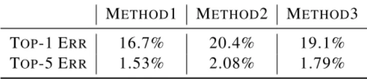
CIFAR-10 and CIFAR-100. CIFAR-10+ and CIFAR-100+ denote to the databases with data augmentation. . . 69 5.4 The learning speed and top-5 classification error (validation set) of

dif-ferent CNNs on ImageNet experiments. . . 70

6.1 The classification error rates of three fine-tune methods on the Pascal VOC 2012 test sets. . . 83 6.2 The time for processing one image of different saliency methods. . . 84 6.3 Fβvalues for differentγ(Pascal VOC 2012, run 35 epochs,β= 0.3). . . 84

6.4 The Fβ value (β = 0.3) of different saliency methods on Pascal VOC

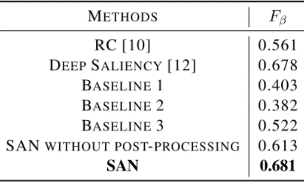
2012 and MSRA10k databases: Aim [8], MISS CB-1 [9], Region Con-trast [10], CNN based Method [11], Deep Saliency [12] and our three kinds of saliency maps . . . 85

(10)

7.1 TheFβ value of different saliency methods on Pascal VOC 2012 (β =

(11)

List of Figures

2.1 Structure of a Deep Neural Network . . . 7

2.2 Sigmoid Function . . . 8

2.3 ReLU Function . . . 8

2.4 An Example of Deep Convolutional Neural Networks . . . 13

3.1 From Left to Right: original images, translated images, rotated images, scaled images and color space translated images. . . 26

3.2 RC works well for simple images (row 1), but can hardly deal with complex images (row 2). In the saliency maps, red means the region has high saliency value, and blue means low saliency value . . . 31

3.3 Multi-context deep saliency can deal with complicated images. . . 32

4.1 Illustration of a hierarchical codebook for AGD . . . 49

4.2 Examples of codewords in hierarchical codebooks of MNIST: Row 1: the second layer of the codebook; Row 2: the third layer of the code-book; Row 3: the fourth layer of the codecode-book; Row 4: the fifth layer of the codebook; Row 5: original training samples . . . 50

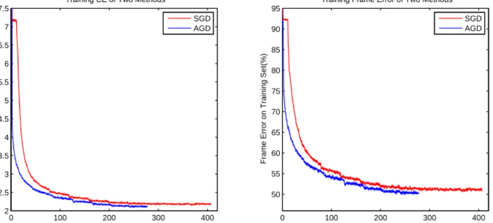
4.3 Learning curves on the MNIST training set (Left: cross entropy error; Right: classification error) of SGD and AGD as a function of elapsed training time. . . 53

4.4 Learning curves on the Switchboard training set (Left: cross entropy error; Right: frame classification error) of SGD and AGD as a function of elapsed training time. . . 54

5.1 The HOPE model is viewed as a hidden layer in DNNs. . . 60

5.2 A convolution layer in CNNs may be viewed as a HOPE model. . . 62

5.3 One HOPE-Block . . . 64

5.4 From Left to Right: Baseline CNN, HOPE-Input CNN, single-HOPE-Block CNN, and multi-HOPE-single-HOPE-Blocks CNN. WhereProjdenotes to one HOPE projection layer,Modeldenotes to one HOPE model layer, and HOPEdenotes to one whole HOPE layer (includes one projection layer and one model layer). . . 66

6.1 The proposed method to generate the object-specific saliency maps di-rectly from CNNs. . . 75

(12)

6.2 Up branch: removing the foregrounds from the input images results in the saliency map with positive salient objects; Down branch: covering the foregrounds of the input images results in the saliency maps with negative salient objects, which may bring about some inefficiency in the post-processing. . . 77 6.3 From left to right: original images, raw saliency maps, smoothed

salien-cy maps and refined saliensalien-cy maps . . . 79 6.4 The PR-curves of different saliency methods on the Pascal VOC 2012

test set (Left) and MSRA10k (Right). . . 86 6.5 Saliency Results of Pascal VOC 2012 (Row 1 to 4) and MSRA10k (Row

5 to 8). (A) original images, (B) ground truth, (C) Region Contrast saliency maps [10], (D) CNN based saliency maps by using [11], (E) multi-context deep saliency method [12], (F) our raw saliency maps, (G) our smoothed saliency maps, (H) our refined saliency maps. . . 87

7.1 The basic structure of the G-Network in GAN. By using fractionally-strided convolutions, the input vector will be converted into several fea-ture maps. The size of feafea-ture maps will gradually increase while the number will decrease. Finally the output is the fake images. . . 91 7.2 The basic structure of the G-Network in SAN. The feature maps’ size

of all layers are same, while the number of feature maps should firstly increase and then decrease. . . 92 7.3 The basic structure of the D-Network in SAN. . . 92 7.4 The whole SAN model that includes the G-Network and D-Network. . . 94 7.5 From left to right: original images, raw saliency maps, smoothed

salien-cy maps and refined saliensalien-cy maps . . . 96 7.6 The configurations of the G-Network and D-Network in our experiments. 98 7.7 Saliency Results of Pascal VOC 2012. (A) original images, (B) ground

truth, (C) Region Contrast saliency maps [10], (D) multi-context deep saliency method [12], (E) Baseline 1, (F) Baseline 2, (G) Baseline 3. (H) the proposed SAN model. . . 100

(13)

List of Acronyms

AGD Annealed Gradient Descent ANN Artificial Neural Network

ASGD Average Stochastic Gradient Descent ASR Automatically Speech Recognition BP Back-Propagation

CE Cross-Entropy

CNN Convolutional neural network CPU Central processing unit DNN Deep Neural Network

GAN Generative Adversarial Network GD Gradient Descent

GMM Gaussian mixture model GPU Graphics Processing Unit HMM Hidden Markov model MCCNN Multi-Colunm CNNs MLP Multi-Layer Perceptron

PCA Principal Components Analysis PER Phone error rate

RBM Restricted Boltzmann Machine

RCNN Recurrent Convolutional Neural Networks ReLU Rectified Linear Unit

SAN Supervised Adversarial Network SGD Stochastic Gradient Descent SVM Support Vector Machine

SVRG Stochastic Variance Reduced Gradient WER Word error rate

(14)

Chapter 1

Introduction

The development of deep learning is a very long story, which can be traced back to 1950s. The presenting of two layer perceptron [13] made the researchers believe that they have revealed the truth of artificial intelligence. However, in 1969, Minsky et al. published a book called Perceptrons [14], in which they prove that perceptrons have some weakness such as cannot express some complicate functions. Moreover, they argued that multi-layer perceptrons (MLP) have no research value because of the lim-itation of computational ability and the lack of learning algorithms. This book can be viewed as an important label of the period called ’AI winter’. In 1980s, Rumelhart et al. presented the famous back-propagation (BP) algorithm [15], which solved some prob-lems of gradient calculation through the introduction of chain rules. Thus the training of MLP became practical. The introduction of hidden layers equip perceptrons with ability of simulate all possible functions [16]. Starting from the BP algorithm, researchers tend to consider neural networks as a mathematical problem instead of biological problem. Even though the BP algorithm brought benefits on the learning of MLPs, it still suffered from low efficiency and many local optima. Moreover, too many hyper-parameters such as learning rate, momentum and number of hidden nodes also obstructed the widely us-age of MLPs. In 1990s, Cortes and Vapnik defined support vector machine (SVM) [17], which showed many advantages compare with MLPs, such as global optimum point, faster learning speed and less hyper-parameters. SVM caused another winter of MLPs, and this situation lasted more than 10 years until the presenting of the fast learn-ing method of deep belief networks [18], where the layer-wise pre-trainlearn-ing technique and network fine-tuning are combined to speed-up the training process. After that, deep learning began to show excellent performance on different tasks such as speech process-ing and computer vision due to the development of computer hardware, especially the

(15)

General-Purpose computing on Graphics Processing Units (GPGPU). GPGPU results in hundreds or even thousands times improvement on the computational performance. Al-so, increasing number of training data are collected for different tasks. And as a result, training deep learning models like fully connected deep neural networks (DNNs) and deep convolutional neural networks (CNNs) from scratch becomes possible. Therefore, currently deep learning models such as DNNs, CNNs, RNNs (Recurrent Neural Net-works) and LSTMs (Long Short Term Memory netNet-works) become an important branch in artificial neural networks (ANNs).

Generally speaking, ANNs are computational models that inspired by an human’s brain systems. It can be described as highly interconnected ”neurons”, which can receive input vectors and output corresponding features. A typical ANN contains three layers: the input layer, hidden layer and output layer. DNNs is the ANNs that contain at least two hidden layers, which may result in more powerful representation ability because the deep structures can extract increasingly abstract features of input data. DNNs serve as an important branch of deep learning, which can be applied to variety application fields.

CNNs [19] is a kind of feed-forward ANNs. A lot of experiments prove that Fully-connected DNNs are powerful for pattern recognition tasks. However, there still re-mains some problems of DNNs especially on computer vision tasks [20], such as the lack of invariance and the deficiency to catch the local features. CNNs are proposed to solve those difficulties. For instance, CNNs provide shift invariance by using weights sharing method and extract local features by using local receptive fields. Therefore, CNNs become the major model for image related tasks.

More recently, DNNs and CNNs not only work well on the classification-related tasks, but also other more complicated tasks. For instance, many computer vision tasks such as image generation [21] and image saliency detection [12] can be addressed by using deep learning models. A lot of researches reflect that DNNs and CNNs have ability to handle more complex features from large amount of training data. However, there are still some challenging research topics in deep learning, such as how to further speed up the training process, how to find a good model to boost the performance, and how to apply deep learning methods more effectively in different tasks.

(16)

1.1

Contributions

This dissertation proposes several novel methods, which include training algorithm, new model and applications, to improve the performance of DNNs and CNNs.

First of all, the dissertation provides a novel DNN training algorithm called Annealed Gradient Descent (AGD) to increase the training speed and prevent the training process from finding some bad local minima. Comparing with the regular stochastic gradient descent (SGD), AGD tries to optimize a low resolution approximation function that de-rives from a group of pre-trained codebooks instead of original training data. Further-more, the approximation resolution is gradually improved according to an annealing schedule over the optimization course. The original non-convex objective function will be optimized at the end of training. This dissertation theoretically proves that AGD can find good optimization results with fast learning speed. The details of AGD algorithm are shown in Chapter 4.

Secondly, the dissertation proposes to use a novel model called Hybrid Orthogonal Pro-jection and Estimation (HOPE) in CNNs for better classification performance. This model introduces a linear orthogonal projection to reduce the dimensionality of the raw high-dimension data and then uses a finite mixture distribution to model the extracted features. By splitting the feature extraction and data modeling into two separate stages, it may derive a good feature extraction model that can generate better low-dimension features for the further learning process. Based on the analysis in [22], this dissertation finds a suitable way to apply HOPE to CNNs and gets state-of-the-art performance on image classification tasks on CIFAR-10, CIFAR-100 [23] and ImageNet [24] databases. Chapter 5 discusses the details of HOPE CNNs.

Besides training algorithm and new model, this dissertation also considers applications of deep learning on image saliency detection, which is a kind of important task in com-puter vision. In Chapter 6, a CNN-based saliency method is presented, which is a much simpler and more computationally efficient method to generate class-specific objec-t saliency maps direcobjec-tly from a well-objec-trained classificaobjec-tion CNN model. This approach use the gradient descent (GD) method to iteratively modify input images based on pixel-wise gradients to reduce a pre-defined cost function. The experimental results show that the CNN-based saliency method can generate high-quality saliency maps in relatively short time (more than 3 times faster than the state-of-the-art deep learning based method in [12]). Chapter 7 precents another novel saliency detection method based on Genera-tive Adversarial Network (GAN) [21], which is called Supervised Adversarial Network

(17)

(SAN). Specifically, SAN also introduces two CNNs: the G-Network is designed to generate synthetic saliency maps from the input images, and the D-Network is used to determine the given saliency map is a synthetic saliency map or a ground truth saliency map. However, different from the regular GAN in [21], SAN applies fully supervised learning method to update both G-Network and D-Network, uses different G-Network structure, and introduces a new type of hidden layer called ’conv-comparison layer’ to make the model more suitable for saliency detection instead of image generation. Ex-periments show that the SAN model can also provide state-of-the-art saliency detection performance on many complex images.

1.2

Outline

In this dissertation, the next two chapters (Chapter 2 and Chapter 3) provide some important background knowledge related to ANNs and image processing. Chapter 4 describes the AGD training algorithm, which includes theoretical analysis and exper-iments. Chapter 5 describes the proposed HOPE CNN model, which firstly describes the basic idea of HOPE and then shows how to apply HOPE on CNNs. Chapter 6 and Chapter 7 presents two different way to apply deep learning models for image salien-cy detection: Chapter 6 shows the CNN-based fast saliensalien-cy method, and Chapter 7 provides the SAN model for saliency detection. Finally, Chapter 8 concludes this dis-sertation and discusses some potential future works.

(18)

Chapter 2

Artificial Neural Networks

Artificial Neural Networks (ANNs) are proposed to simulate the natural human brains for good pattern recognition ability. They can be described as highly interconnect-ed ”neurons” which can receive input vectors and output the corresponding features. In 1943, Warren McCulloch and Walter Pitts proposed a computational model called threshold logic, which can be viewed as an early prototype of ANNs [25]. Their re-search showed that ANNs are a kind of potential tools to implement artificial intelli-gence. In 1958, Frank Rosenblatt proposed the basic idea of perceptron, which is a two-layer neural network (one input layer and one output layer) with linear connec-tion [13]. In later 1980s, the development of the famous back-propagaconnec-tion algorithm [15] make it possible to train multi-layer ANNs such as multi-layer perceptron(MLP). Moreover, by using non-linear activation functions such as sigmoid and relu, multi-layer perceptron has been proved that it has ability to approximate all possible functions in real-world [26]. However, because of the insufficiency of the computational perfor-mance and lack of training data, training large scale ANNs (e.g. DNNs and CNNs) was impractical. Fortunately, in 2007, NVIDIA released the first edition of CUDA. CUDA is a GPU based parallel computing toolkit, which enables researchers to use GPU for general purpose computing. This brings about hundreds times speed-up in the training of ANNs. Moreover, some large-scale databases such as ImageNet [24] and COCO [27] are released, which can help the learning of deep models. Therefore, ANNs begin to going deeper and deeper and yield excellent performance in variety of applications.

Recently, deep learning has achieved significant successes in many real-world applica-tions, such as speech recognition and computer vision. It becomes a very interesting problem to learn large-scale deeply-structured ANNs, such as DNNs and CNNs, from

(19)

big databases. Deep learning algorithms can detect both low-level and high-level fea-tures from the input data automatically, and as a result, they may have excellent perfor-mance in practice.

When learning deep models, the back-propagation algorithm, sometimes being com-bined with layer-wise greedy pre-training, is the most important training method. The back-propagation algorithm collects error signals from the output layer by comparing network outputs and training targets and back-propagates the error signals layer-by-layer to efficiently derive gradients with respect to all network weights. The weights are then updated by using the gradient descent algorithm. However, since deep models are highly non-convex in nature, the learning process may finally result in a bad local optima. Moreover, since the deep models contain a large number of free parameters, a finite size training set may lead to over-fitting. A lot of efforts aim to deal with those problems, such as data augmentation, dropout, and the proposed AGD algorithm in this dissertation.

This chapter reviews two famous deep learning models: DNNs and CNNs, as well as their training methods and applications.

2.1

Deep Neural Networks

Deep Neural Networks (DNNs) is the fully-connected ANNs that contain at least two hidden layers (see an example in Figure 2.1), which may result in more powerful repre-sentation ability because the deep structures can extract increasingly abstract features of input data. DNNs serve as an important branch of deep learning, which can be applied in variety application fields. This section reviews the basic model of DNNs and their training algorithm, and also discuss some applications.

2.1.1

Basic Model

[28] provides the basic computational model of DNNs. Assuming that a DNN has L hidden layers, and given an input vector x, then some important notations can be defined:

(20)

FIGURE2.1: Structure of a Deep Neural Network

2. zl_{: the output of the} _{lth hidden layer, and} _zl ₌ _f₍_al₎_{, where} _f₍_·₎ _{is a non-linear}

activation function

3. al: the activation of thelth hidden layer, andal =Wlzl−1+bl−1

4. o=zL+1_{: the final output of the DNN, and}_o₌_{sof tmax}₍_aL+1₎

where the definition of the softmax function is:

sof tmax(x) = _Pexp(x)

jexp(x)

(2.1)

For the hidden layers, an activation function f(·) should be pre-defined. One well-known and successful activation function is sigmoid function (see Figure 2.2):

f(x) = 1

1 +e−x (2.2)

Using sigmoid function needs to carefully fine-tune some hyper-parameters including learning rate, momentum and mini-batch size to get the best performance. More impor-tantly, for deep models, applying sigmoid function may result in the problem of gradient vanishing.

Currently, a novel activation function called rectified linear unit (ReLU) [1] is becoming increasingly prevalent. The form of ReLU isf(x) = max(0, x), which is much simpler than the standard sigmoid function. Using ReLU may increase the training speed of DNNs because its gradient can be calculated much easier (Figure 2.3). Moreover, large number of experiments suggest that ReLU DNNs allow to use much larger mini-batch

(21)

FIGURE2.2: Sigmoid Function

size to get excellent performance, while sigmoid function requires smaller mini-batch size [29]. This means that the ReLU DNNs can be parallelized much easier by intro-ducing GPU computing or mulit-CPUs.

FIGURE 2.3: ReLU Function

Furthermore, He et al. proposed a generalization of ReLU, i.e. Parametric Rectified Linear Unit (PReLU), to further increase the performance of ReLU [30]. Compare with regular ReLU, PReLU has a different definition when the inputxless than zero:

f(x) =    x x≥0, ax x<0. (2.3)

(22)

whereais a learnable hyper-parameter. Comparing with the constantain Leaky ReLU (LReLU) in [31], PReLU is more flexible and has slightly better performance on many databases.

2.1.2

Network Training

DNNs can be trained to optimize the cross-entropy (CE) criterion, which measures the difference between the desired labels and the actual outputs calculated by DNNs, and the standard error back-propagation algorithm can be applied through Stochastic Gradi-ent DescGradi-ent (SGD). By merging the biasbl_{into the weight matrix}_Wl_{, only the iterative}

updating rule ofWlneed to be considered by using gradient information as below:

Wl=Wl−λ∂FCE

∂Wl , (1< l < L+ 1) (2.4)

whereλis the learning rate.

For any input vector x, the output of a given DNN is calculated using the softmax function as follows: ont = Pr(tn|xn) = eaLnt+1 P t0ea L+1 nt0 (2.5)

where aL_nt+1 denotes the activation signal at the output layer corresponding to the nth training sample pair and the output labeltn. Assuming that the whole training set

con-sists of all training samples and their corresponding target labels, the CE objective func-tion can be expressed as the following form:

FCE(W) =− N X n=1 log Pr(tn|xn) = − N X n=1 logont (2.6)

whereW denotes all connection weights in the DNN, and on is the output at the top

softmax layer given the input vectorxn.

In the standard back-propagation (BP) algorithm, the most important quantities need to be calculated are the gradients of the CE objective function with respect to the input

(23)

activations,al

j, at each layer, which are normally called aserror signals:

el_nj ≡ − ∂ ∂al

j

log Pr(tn|xn). (2.7)

For the CE objective function in Eq. (2.6), the error signals at the output layer can be computed as:

eL_nt+1 =−∂logont ∂ant

=ont−δnt (2.8)

whereδnt = 1 ift equals to the target label tn and otherwise δnt = 0. And the error

signals for all other layers (1≤l ≤L) can be calculated fromel_nt+1following a standard error back-propagation procedure as follows:

el= (Wl+1)0el+1· ∇zl (l =L, ...,1) (2.9) where the vectorel _{is constructed by concatenating all error signals in layer}_l, _·_stands

for the element-wise multiplication between two vectors with the same size, and ∇ means to calculate the gradients.

Once all error signals for all nodesj in all layerslgiven each input vector are provided, the gradients for all DNN weights can be easily derived from these error signals. In this case, the gradients with respect to all DNN weights can be easily obtained as:

∂FCE(W)

∂Wl =e

l_∇_zl−1 ₍_∀_l₎

(2.10)

Substituting Eq. (2.10) into Eq. (2.4), all DNN weights can be updated iteratively based on SGD algorithm.

However, training DNNs by using back-propagation is a difficult task. In [32], Erhan et al. argue that one important challenge of training deep models is that the objective functions are always highly non-convex. Therefore, it may exist numerous local mini-mum points, and the gradient based learning algorithm may easy to get stuck into bad local optima. Applying SGD may help to relieve this situation, since the random noise introduced by each training sample may help the algorithm to escape from some bad local minima, but the random noise may also slow down the learning speed.

(24)

One possible way to deal with this difficulty is to initialize the DNNs by using greedy layer-wise pre-training under some unsupervised criterions [28], where Restricted Boltz-mann Machines (RBMs) or auto-encoders can be employed. A hypothesis that can ex-plain the effects of unsupervised pre-training is proposed in [32]. In this paper, Erhan et al. present that the pre-training procedure can restrict the model parameters inside a relatively small region of parameter space, which corresponds to capturing structure of the input distributionP(x)in each layer, and those information catched by pre-training process can serve as a good initialization for the further supervised fine-tuning. The experiments show that unsupervised pre-training is robust to the random initialization and can provide the DNNs with better generalization performance.

Another potential weakness of DNNs training is over-fitting. The increasing number of hidden layers cause more and more adjustable model parameters, and over-fitting then becomes easier to happen. Even though some strategies like early stopping and regu-larization schemes can be used to prevent over-fitting, it still remains a major challenge when training some extremely large DNNs with relatively small size training set. Model combination is a good method to relieve over-fitting. Unfortunately, training large-scale DNNs is time-consuming, and as a result, training several DNNs for model combination often becomes impractical. To deal with those problems, previous researchers proposed dropout method [33].

The basic idea of dropout is to randomly drop each unit in a DNN with probability p (p= 0.5for example), and ”drop” means that remove the unit and its related edges from the network. During the training process, dropping out should be done independently for each hidden unit and for each training sample. As a result, dropout can be regarded as a sub-sampling of the DNN, and a DNN with n hidden units can be viewed as a collection of2n_{possible weight shared sub-DNNs.}

When dropout is combined with DNN training, the feed forward operation can be de-fined as below: rl_i ∼Bernoulli(p) ˜ zl =rl·zl al+1 =Wl+1z˜l+bl+1 zl+1 =f(al+1) (2.11)

whererlis a vector that contains Bernoulli random variables to determine that whether one node in layer l should be dropped, and each element in rl _{has probability} _p _of

(25)

equaling to 1. During the learning, the gradient of the loss function should be back propagated through the dropped network.

In the test phase, the DNN weights need to be re-scaled: Wtest = pW. The purpose

of this operation is to approximate the average over all possible dropped network. By doing this, the dropout DNNs can share some advantages of model combination method.

In [1], Dahl et al. combine rectified linear activation function and dropout during the DNN training, and provide experiment results on DARPA EARS database, which con-tains 50 hours English broadcast news data. The test results are listed in Table 2.1. This table implies that dropout combine with rectified linear can provide better performance even though without pre-training.

TABLE2.1: Performance on DARPA EARS Database [1]

ACTIVATIONFUNC PRE-TRAINING DROPOUT TRAININGERR TESTERR

RECTIFIEDLINEAR YES YES 10.7% 18.5%

RECTIFIEDLINEAR NO YES 11.0% 18.9%

SIGMOID YES NO 11.3% 19.4%

Based on dropout, several generalization methods have been presented. Wan et al. de-signed dropconnect algorithm in [34]. Instead of dropping a subset of units, dropcon-nect randomly selects some elements in the weight matrices and set them to 0. Ex-periments on some databases show that dropconnect can provide better performance compare with regular DNNs and even dropout. In [35], an adaptive edition of dropout called standout is proposed, and the basic idea is to overlay a binary belief network on the DNN and use it to regularize the hidden units by selectively setting activities to 0. This overlaid belief network can be trained during the DNN training. The experiments show that standout can also provide lower error rate than standard dropout.

2.2

Deep Convolutional Neural Networks

Convolutional Neural Networks (CNNs) [19] also belong to feed-forward ANNs. As this dissertation mentioned before, the fully-connected DNNs are powerful when doing pattern recognition tasks. However, there are still some problems of DNNs especially when deal with image processing tasks [20].

(26)

Firstly, typical images (grey-scale or color images) may corresponding to large input features, which will obviously increase the size of weight matrices, and then may lead to over-fitting problem and require more memory resources. These difficulties sometimes make the DNNs become impractical in real-world image-related applications.

Secondly, the fully-connected DNNs are short of invariance of translations and local distortions of the input features. Even though pre-processing of input images can be performed to provide some invariance, they are far from perfect and may easy to cause variations of the inputs. It is true that increasing the size of DNNs may handle those variations, but it requires large number of training samples and memory size, and also makes the training process much slower.

Thirdly, images have a lot of 2D local structures, but this kind of local features cannot be reflected in fully-connected DNNs because the input order of DNNs cannot affect the network output, and this may also bring about negative impacts on the recognition performance.

CNNs are proposed to solve those difficulties. For instance, CNNs can provide shift invariance by using weights sharing technique and can extract local features by using local receptive fields.

2.2.1

Basic Model

A typical CNN has three kinds of layers: convolutional layers, pooling layers and fully-connected layers, and in most cases one or more convolutional layers and one pooling layer can be grouped as one block (see Figure 2.4 as an instance).

FIGURE2.4: An Example of Deep Convolutional Neural Networks

(27)

As Figure 2.4 show, one convolutional layer of CNNs may contain several feature maps, and each feature map is related to a local receptive field, which scans the previous layer and receive signals from local areas. Obviously, this operation is equivalent to a convolution with a small size window [19]. In addition, images have a property that one specific pattern may appear in the entire image. To utilize this nature, the weight sharing technique is introduced in each feature map, which means that the same weights will be used to process all local regions in the input feature maps. Another benefit of weight sharing is that it can significantly reduce the number of free parameters.

To compute the output of one feature map, the convolution kernel w with the size k should be defined at first, and then the output of thelth layer can be calculated as below:

al_x,y =wl_x,y∗hl_x,y+bl_x,y

= k−1 X x0₌₀ k−1 X y0₌₀ wl_x0_,y0f(a_xl−₋1_x0_,y₋_y0) +bl_x,y (2.12)

wheref denotes a pre-defined activation function (which is similar as DNNs), andx, y have the range0< x < k−1and0< y < k−1are the range that pixels are defined. For the undefined pixels, the zero-padding can be used to make the output feature map has the same size as input.

2. Pooling Layers

To increase the robustness of CNNs, one possible way is to reduce the resolution of higher layers because it can make CNNs tolerate to a slight distortion or translation in the input features [19]. Therefore, pooling layers can be used after one or more convolutional layers to do down-sampling and then reduce the resolution of the feature maps. The pooling layers perform down-sampling by using a small pooling window and calculate one single value to replace all values inside the window, thus it generates smaller feature maps than the previous convolution layer.

In practice, two kinds of pooling functions are usually used: maximum pooling and average pooling [7]. The maximum pooling function function is defined in Eq. (2.13):

pi,j = G max m=1 G max n=1 q(i−1)×s+m,(j−1)×s+n (2.13)

where i and m are the index in one feature map, G is the pooling size, and s is the shift size that control the overlap of adjacent pooling windows. Similarly, the average

(28)

pooling function can be defined as below: pi,j =r G X m=1 G X n=1 q(i−1)×s+m,(j−1)×s+n (2.14)

whererdenotes a scaling factor.

The pooling layers in CNNs may be viewed as a feature extraction procedure, which extract the most prominent signal component within a small neighbouring region. The pooling layers, using either average pooling or max pooling, are critical in CNNs [36] since they can make the models more tolerable to the slight distortion or translation in the original images [19]. In [37], a theoretical analysis of average pooling and max pooling is made to reflect how pooling can affect the network performance. However, in most cases, pooling layers are still used based on empirical information.

3. Fully Connected Layers

To further improve the performance of CNNs, several fully connected layers can be applied upon the convolution layers and pooling layers. The structure of the fully con-nected layers are identical with regular DNNs.

2.2.2

Network Training

Similar with DNNs, error back-propagation algorithm can also be used to train CNNs. Because of the existence of pooling layers and the usage of weight sharing, the back-propagation needs some small modification. When propagating error signals through a pooling layer, the kind of pooling function should be considered. For example, for the maximum pooling function, only the signal that passed the most active unit in each group of the pooled units should be kept [7].

To update the shared weights in one convolution kernel, the weights updates over all units in the corresponding feature maps should be collected. Specifically, the gradient of the error signal E with respect to the convolution kernel of thelth layer wl _{can be}

calculated as below: ∂E ∂wl x,y = k−1 X x0₌₀ k−1 X y0₌₀ ∂E ∂al x0_,y0 ∂al_x0_,y0 ∂wl x,y = k−1 X x0₌₀ k−1 X y0₌₀ δl_x0_,y0 ∂al_x0_,y0 ∂wl x,y (2.15)

(29)

By doing some simple transformation, ∂a l x0,y0

∂wl

x,y can be re-written as:

∂al x0_,y0 ∂wl x,y = ∂ ∂wl x,y ( k−1 X x00₌₀ k−1 X y00₌₀ w_xl00_,y00f(a_xl−0₋1_x00_,y0₋_y00) +bl) = ∂ ∂wl x,y (wl_x,yf(a_xl−0₋1_x,y0₋_y)) =f(al −1 x0₋_x,y0₋_y) (2.16)

Therefore, Eq. (2.15) can be re-written as:

∂E ∂wl x,y = k−1 X x0₌₀ k−1 X y0₌₀ δ_xl0_,y0f(a_xl−0₋1_x,y0₋_y)

=δ_x,yl ∗f(al₋−_x,1₋_y) =δ_x,yl ∗f(rot180◦(al_x,y−1))

(2.17)

whererot180◦ means to rotate the matrix for 180 degrees. In Eq. (2.17),δl

x,y is defined

as _∂a∂El

x,y. Again, by using chain rules, it can be expressed as:

∂E ∂al x,y = k−1 X x0₌₀ k−1 X y0₌₀ ∂E ∂al_x+10_,y0 ∂al_x+10_,y0 ∂al x,y = k−1 X x0₌₀ k−1 X y0₌₀ δ_xl+10_,y0 ∂al_x+10_,y0 ∂al x,y (2.18)

Similar with Eq. (2.16), the term ∂a l+1

x0,y0

∂al

x,y can be re-written as:

∂al_x+10_,y0 ∂al x,y =wl_x+10₋_x,y0₋_y ∂ ∂al x,y (f(al_x,y)) (2.19)

Then subsituting Eq. (2.19) into Eq. (2.18):

δ_x,yl = k−1 X x0₌₀ k−1 X y0₌₀ δ_xl+10_,y0w_xl+10₋_x,y0₋_y ∂ ∂al x,y (f(al_x,y)) =δ_x,yl+1∗rot180◦(wl+1 x,y) ∂ ∂al x,y (f(ol_x,y)) (2.20)

(30)

Eq. (2.17) and Eq. (2.20) implies that the back-propagation of CNNs can also be viewed as a convolution procedure, which helps the implementation of CNNs.

Some techniques like unsupervised pre-training and dropout can also be used to further increase the performance of CNNs. Furthermore, Ossama et al. [7] proposed a limited weight sharing (LWS) method for CNNs that make them can work well with speech recognition tasks. Different with the weight sharing over the whole feature map, LWS only forces the weights of the same group of pooled units to be identical.

2.3

Applications

This section briefly reviews some applications of ANNs, and the selected applications can be divided into two parts: image processing and speech processing.

2.3.1

Image Classification Tasks

In [2], Ciresan et al. implemented DNNs on CUDA platform, and the utilization of GPU parallel computing significantly accelerate the training speed of DNNs. In exper-iments, DNNs are used to solve the hand-written digits classification. MNIST database is a well-known handwritten digital images database, which contains 60000 training samples and 10000 test samples (The gray-scale hand-written digits are much simpler compare with RGB natural images thus can be handled by fully-connected DNNs). However, when using the deep architecture, the training sample size of MNIST is too small to prevent over-fitting. Instead of applying unsupervised pre-training, this paper considers to expand the training sample size by using image augmentation methods. Specifically, 4 kinds of randomly augmentations (rotation, scaling, horizontal shearing and elastic deformation) are introduced, and the image augmentation methods should be executed at the beginning of each training epoch. And as a result, the DNNs can almost never see the same training sample twice during the training procedure. The test results listed in Table 2.2 reflect the excellent performance of the proposed method. In this table Architecture indicates the number of hidden layers and the size of each hidden layer.

In [38], Ciresan et al. proposed a noval multi-column CNNs to further improve the image classification performance of deep architectures. In this paper, the proposed C-NN contains hundreds of feature maps in each layer, and using maximum pooling as

(31)

TABLE2.2: Average Test Error and Best Test Error of DNNs with Different Network Configurations on MNIST Database [2]

ARCHITECTURE AVERAGE BEST TRAININGTIME

1000, 500 0.49% 0.44% 23.4(hr)

1500, 1000, 500 0.46% 0.40% 44.2(hr)

2000, 1500, 1000, 500 0.41% 0.39% 66.7(hr)

2500, 2000, 1500, 1000, 500 0.35% 0.32% 114.5(hr)

the down-sampling method. The main difference with the regular CNNs is that several columns of CNNs are combined and construct the so called multi-colunm CNNs (MC-CNNs). Before training, all columns of CNNs are initialized randomly, and then each column can be trained by using the same inputs, or inputs that derived from various pre-processing methods. Finally the outputs of each columns should be averaged to get the final classification results. Because of the acceleration provided by GPUs, the training of several colunms of CNNs can be done in relatively short time. On MNIST database, MCCNNs achieve 0.23% error rate, which is even better than DNNs that mentioned before. Furthermore, this method has been used to deal with some real-world problem-s like traffic problem-sign claproblem-sproblem-sification [39] and alproblem-so achieveproblem-s excellent performance (99.46% average recognition rate).

In ILSVRC-2012 competition, Krizhevsky et al. [40] proposed to use a deep CNN to classify the ImageNet database, which contains 1.2 million high-resolution images. The proposed CNN includes 5 convolutional layers and 2 fully-connected layers. To reduce overfitting, data augmentation and dropout are applied during the training process. On the test set of ImageNet, the proposed CNN achieves15.3%top-5 error rate. Comparing with traditional image classification algorithms such as Fisher Vectors [41] (26.2% top-5 error), the proposed CNN has much better classification performance.

In [42], a novel CNN model called All-CNN is defined. This model proposed to use regular convolutional layers with larger stride to replace the original pooling layers for better performance. This modification introduces more learnable parameters into the network, and reduces the classification error on CIFAR-10 test set (9.08% vs 9.47%, without data augmentation).

Instead of removing pooling layers from CNNs, [43] proposed to generalize the pooling functions. Based on the traditional average pooling, denote byfavg(x), and maximum

(32)

pooling, denote byfmax(x), two novel pooling methods, i.e. mixed max-average

pool-ing and gated max-average poolpool-ing, are presented. The definition of mixed max-average pooling is:

fmix(x) = afmax(x) + (1−a)favg(x) (2.21)

where a is the weight of two pooling methods and can be learned via BP algorithm. Gated max-average pooling has more complicated form, which introduces learnable gating maskwand sigmoid activation function instead of scalar weightain Eq. (2.21):

fgate(x) =sigmoid(wTx)fmax(x) + (1−sigmoid(wTx))favg(x) (2.22)

The gating maskwcan also be learned by using BP algorithm. Finally, the tree-pooling method can be defined based on gated max-average pooling. Specifically, several pool-ing filters are used to generate the leaf nodes of tree-poolpool-ing. Then every two leaf nodes can be combined by using Eq. (2.21). This process continues layer-by-layer until the root of the tree is generated. The experimental results show that the tree-pooling method achieves state-of-the-art performance on CIFAR-10 test set (7.62% error rate without data augmentation and6.05%with data augmentation).

CNNs can also be used in the field of object detection. In [3], a CNN based algorithm called DetectorNet is presented to locate the bounding boxes of objects in given im-ages. The network structure applied for DetectorNet includes five convolutional layers and two fully connected layers. Each layer uses ReLU as the activation function, and maximum pooling is used as down-sampling method. The main difference between DetectorNet and standard CNNs is that in DetectorNet a regression layer is utilized as the top layer instead of a softmax layer to generate the object binary masks, which can represent the location of objects. By resizing the image, the output binary mask may represent one or more objects. Moreover, this work proposed DNN-generated Masks to further improve the detection performance. In experiments, the DetectorNet is com-pared with several other object detectors on Pascal VOC 2007 database, and it shows state-of-the-art performance of various classes. The test results are shown in Table 2.3. However, one drawback of this method is its relatively high computational cost at train-ing time because the network should be trained for each object type and mask type. Therefore, the future work should aim to train a single network to detect different class-es of objects.

(33)

TABLE 2.3: Average Precision of DetectorNet and Other Methods on Pascal VOC 2007 Database [3]

OBJECTCLASSES BIRD BUS CAT COW TV DETECTORNET 0.194 0.532 0.272 0.348 0.470 SLIDINGWINDOWS 0.068 0.294 0.101 0.131 0.119 3-LAYERDNN 0.094 0.440 0.213 0.193 0.393 DPM APPROACH 0.107 0.513 0.179 0.240 0.413

Scene labeling is a task that aims to label a given image pixel-by-pixel based on the classes of objects. This task is also an important branch in image processing. CNNs can be used to solve this problem. In [4], a modified CNN model named recurrent convolutional neural networks (RCNN) is proposed to do scene labeling and achieved outstanding performance with good efficiency. Recurrent means that its architecture consists of several instances of regular CNNs, and all instances share the same model parameters. The experiments results are provided in Table 2.4, which proves that RC-NNs have both good accuracy and fast execution speed. This research illustrates that the scene labeling tasks can be solved effectively and efficiently without use of expensive graphical model or segmentation methods, and can achieve state-of-the-art performance with fast inference time.

TABLE 2.4: Performance of RCNN and Other Methods on Stanford Background Database [4]

METHODS PIXELACCURACY(%) COMPUTINGTIME(S)

ALGORITHM IN[44] 76.4 10TO600

ALGORITHM IN[45] 81.9 >60

REGULARCNN 79.4 15

RCNN (2INSTANCES) 76.2 1.1 RCNN (3INSTANCES) 80.2 10.7

2.3.2

Speech Recognition Tasks

In the past few years context-dependent DNN-HMM (Hidden Markov Model) hybrid model achieves significant success in the field of automatical speech recognition (ASR). Different from the traditional GMM-HMM ASR system, DNNs serve as the acoustic models to generate the posterior probabilities of HMM states, and then HMM is used to do decoding and get the recognition results. In [5], a noise robust DNN-HMM system

(34)

is proposed by combining DNNs with several noise robustness methods include multi-condition training data, enhanced feature, model adaptation and dropout. Experiments on Wall Street Journal (WSJ0) database can reflect the performance of the noise robust system. Specifically, the multi-condition training set of WSJ0 contains7137utterances from 83 speakers, and the test set can be divided into 4 groups: clean, noisy, clean with channel distortion and noisy with channel distortion (denote by A, B, C, and D respectively). These four kinds of test sets are used to evaluate the robustness of the al-gorithm. Two kinds of input features for DNN-HMM and the baseline GMM-HMM are applied: MFCC and FBANK-24. Table 2.5 reflects that DNN-HMM shows better per-formance and robustness compare with GMM-HMM. Specifically, DNN-HMM model can work well with noisy data, and the utilize of FBANK-24 features further increase the recognition accuracy.

TABLE 2.5: Word Error Rate (%) of GMM and DNN Acoustic Model on WSJ0 Database [5]

METHOD/FEATURES A B C D AVERAGE

GMM-HMM(MFCC) 12.5 18.3 20.5 31.9 23.0 DNN-HMM(MFCC) 5.7 10.4 10.9 22.6 15.3 DNN-HMM(FBANK-24) 5.0 9.2 9.0 20.6 13.8

In [6] and [46], a multiple DNNs (mDNNs) acoustic model is presented to replace the standard single large scale DNN to compute the states posterior probabilities. During the training phase, all tied states of context-dependent HMMs are firstly divided into some clusters, and then several DNNs are trained by using those clusters respectively in parallel. The outputs of the multiple DNNs can be combined to calculate the pos-terior probabilities for decoding. Table 2.6 shows that the mDNN-HMM model brings about significant acceleration (over 7 times acceleration with 4 GPUs) with negligible performance hit. Thus this model is practical for large-scale ASR tasks.

TABLE2.6: Word Error Rate (%) of DNN and mDNN Acoustic Model on Switchboard Database [6]

#OFHIDDENLAYERS 3 4 5 6

DNN-HMM WORDERR 17.7 16.9 16.4 16.2 EXECUTIONTIME(hr) 11.0 13.0 13.6 15.0 MDNN-HMM WORDERR 17.8 17.0 16.9 16.7 EXECUTIONTIME(hr, 3 GPUS) 3.0 3.7 4.3 5.0

(35)

TABLE2.7: Performance of CNNs and DNNs with Different Configuration on TIMIT Database [7]

NETWORKSTRUCTURE AVERAGEPER(%)

DNN (2000 + 2∗1000) 22.02 DNN (2000 + 4∗1000) 21.87 CNN (LWS(M:150P:6S:2F:8)+2∗1000) 20.17 CNN (FWS(M:300P:6S:2F:8)+2∗1000) 20.31 CNN (FWS(M:150P:4S:2F:8)+FWS(M:300P:2 S:2F:6)+2∗1000) 20.23 CNN (FWS(M:150P:4S:2F:8)+LWS(M:150P:2 S:2F:6)+2∗1000) 20.36

Ossama et al. proposed a modified CNNs that can also work with ASR problems [7][47]. In this research, the input data should firstly be re-organized to make them compatible with the CNN structure. For instance, the input features can be arranged as three 2D feature maps, each of which represents the original data, first-order derivative and second-order derivative respectively. Each feature map contains several adjacen-t frames and adjacen-the re-organized feaadjacen-tures maps can be feed inadjacen-to adjacen-the CNN. Moreover, adjacen-to make the CNN more suitable for ASR tasks, the limited weight sharing (LWS) method is proposed instead of the traditional fully weight sharing (FWS). TIMIT database is used to evaluate (using phone error rate (PER) to measure the performance) the pro-posed method, and the results of different configurations are presented in Table 2.7, where ’m’ is the number of feature maps, ’p’ is the pooling size, ’s’ is the shift size, and ’f’ is the filter size. The experiments implies that CNNs can provide about6−10%

relative error reduction compare with fully-connected DNNs. Moreover, the applying of LWS scheme makes the CNNs more suitable to deal with ASR tasks.

(36)

Chapter 3

Image Processing

Image Processing is an important research field in computer vision. Recently, increasing number of works begin to consider to apply deep learning algorithms to solve the image processing related problems, which may include image classification, object localiza-tion and deteclocaliza-tion, image saliency deteclocaliza-tion and segmentalocaliza-tion, and image generalocaliza-tion. CNNs become one of the most important tool for those variety of tasks. This chapter will review several important tasks in image processing.

3.1

Image Pre-Processing

When using CNNs to deal with image processing tasks, it may not be a good choice to directly use the original image (gray-scale, RGB or other color channels) as the input feature, since the raw features may be too complicated and noisy for the deep learning systems. Moreover, most of the commonly-used image datasets suffer from the lack of training samples. For instance, Pascal VOC 2012 [48] has only5717training images, and MNIST has only 60000 training samples. The insufficient training samples may lead to over-fitting when train large scale CNNs. All of the facts above imply that some pre-processing methods are required for image processing tasks. This section will review some important pre-processing methods, which include image whitening, image data augmentation and superpixel segmentation.

(37)

3.1.1

Image Whitening

Whitening transformation is a kind of linear transformation that transform the input signals to white noises. The main idea of the whitening transformation is to convert a sequence of random variables to another new sequence with an identity covariance matrix [49]. The identity covariance matrix implies that the new random variables are de-correlated and have variance of 1.

In the natural images, the adjacent pixels are always have high correlation, which may bring about a lot of redundancy in the image information. Doing image whitening can remove those correlation and help the learning algorithm to extract the independent information from the training data.

Assume that there is a training set X ∈ Rn×m (all features have zero mean value), wherenis the feature dimension andmis the sample size. Then the covariance matrix of the training data is:

Σ = 1

mXX

T

(3.1)

Then the singular value decomposition onΣcan be done as Eq. (3.2) shown:

[U, S, V] =svd(Σ) (3.2)

whereU is the eigenvector matrix ofΣ,S is the eigenvalue diagonal matrix, andV =

UT _(because_Σ_{is a symmetric matrix). Then it is easy to know that}_{Σ =}_{U SV}_.

Based on Eq. (3.1) and Eq. (3.2), the definition of PCA whitening is:

XP CA =S 1 2UTX =     1 √ λ1 ... 0 0 ... 0 0 ... _√1 λn     Xrot (3.3)

whereXrot =UTX denotes to rotateXto the basis of all eigenvectors. Then it is very

easy to derive thatΣP CA =I, whereI denotes the identity matrix.

Based on the definition of PCA whitening, it is easy to define ZCA whitening:

XZCA =U XP CA (3.4)

which can be viewed as transform the PCA whitened data back to the original feature space. Also, it is easy to verify thatΣZCA =I.

(38)

Experimental results show that using ZCA image whitening on CIFAR-10 database can improve classification accuracy on relatively small-scale CNNs. However, for deep CNNs, ZCA whitening cannot bring obvious benefits. One potential reason is that deep networks can already gradually de-correlate features.

3.1.2

Image Data Augmentation

Even though the number of free parameters in CNNs has been significantly decreased by using local receptive fields and weight sharing, training deep CNNs still requires huge number of training data. However, when using supervised learning, the well-labeled training data are always far from enough. Therefore, data augmentation becomes an im-portant pre-processing for image processing tasks. In practice, even ImageNet dataset (around 1.4 million training images) [24] also needs to be augmented to train very deep neural networks such as vgg nets [50] and deep residual nets [51]. The simplest way of image data augmentation is image fliping. For instance, [52] proposed a deep neural network for CIFAR-10 [53] image classification. The author argues that when randomly do horizontal flip for 50% images on the training set, the classification accuracy on test set improves from 91.30% to 92.45%. In [54], more complicate image data augmenta-tion methods are considered to improve the classificaaugmenta-tion performance of CNNs on the ImageNet database . The paper mainly focus on the so-called key augmentations, in-cludes color casting, vignetting, stretch and cropping and lens distortion. In Chapter 5 of this dissertation, four kinds of image augmentations are also used for better clas-sification performance on both CIFAR-10 and CIFAR-100 databases, i.e., translation, rotation, scaling and color space translation. Figure 3.1 displays some examples of the selected data augmentation.

3.1.3

Superpixel

Superpixel segmentation is another important image pre-processing method for image processing tasks. Superpixel is a image region that has perceptually uniform feature, which can be viewed as an over-segmentation of images. For the digital images, pixel-grids are the basic units, and most computer vision algorithms may use them as the input data. However, in some cases, simply using raw pixels has some drawbacks. Pixel-grid itself is not a natural way to represent images. It simply divides natural im-ages into large number of pixels and dispatches RGB values (or other color channels

(39)

FIGURE 3.1: From Left to Right: original images, translated images, rotated images, scaled images and color space translated images.

like YUV) to each pixel based on the corresponding color information. This may lead to some disadvantages in practice. Firstly, pixel-grids cannot reflect the some high-level information of images, such as different objects or some regions with similar color/tex-ture feacolor/tex-tures. Secondly, currently most images have high resolution, which means that they may include huge number of pixel-grids. For example, one 300-by-500 image has 150,000 pixels, which may significantly increase the computational complexity. There-fore, some superpixel algorithms are proposed to group several adjacent pixels that share the similar color or texture into one superpixel to reflect some high-level feature and reduce the complexity of the images (from hundreds of thousands to around one hundred) without losing useful feature [55]. Superpixels can be applied to different kinds of applications such as video objects tracking [56], image saliency detection [57] and segmentation [58].

There are a lot of superpixel extraction algorithms proposed in previous researches. In [59], superpixel segmentation is used as an important pre-processing for the final image segmentation. In this paper, Normalized Cuts [60] algorithm combined with contour

(40)

and texture features are used to generate superpixel maps. The experiments show that most superpixels have similar size and shape, and can keep most important features and structures in the input images. Those facts can help the further segmentation.

In [61], the Entropy Rate Superpixel Segmentation method is proposed. This method introduces a novel objective function that contains two components to guide the super-pixel generation. Specifically, the algorithm uses undirected graphs to represent images, and introduces a random walk process on the graphs. The first term of the objective function is defined as the entropy rate of the random walk. Based on the definition of the entropy rate term, it encourages compact and homogeneous superpixels. The second term is the balancing term, which makes all superpixels tend to have similar size. By using greedy optimization, the algorithm can generate superpixels with similar size and keep the object boundaries.

Seeds algorithm [62] is another superpixel extraction method that uses a simple hill-climbing optimization method to reduce the computational costs. Different with most of the superpixel algorithms, Seeds starts from an initial superpixel partition (for exam-ple dividing the original images by using regular grids), i.e., some seeds, and gradually modify the superpixels by changing the boundaries. To guide the boundaries changing process, a robust energy function is proposed based on the color distribution inside the superpixels (the color distribution term) and the shape of the superpixels (the bound-ary term). The hill-climbing optimization means that in each iteration some small local changes of the superpixels will be proposed, and if the energy function increases, the superpixel partition will be updated. Experimental results show that after several itera-tions good superpixel maps can be generated.

Simple Linear Iterative Clustering (SLIC) [63] is also a well-know superpixel genera-tion method, which based on K-means clustering algorithm and can provide state-of-the-art performance on different image databases. Specifically, SLIC can be divided into three steps:

(1) Initialization: assuming that the image size isN×N, and the expectation number of superpixels isk. The algorithm tends to generate homogeneous sized superpixels with the approximate sizeS×S. Obviously,Sshould roughly equals toN/√k. Therefore, similar with Seeds algorithm, SLIC firstly splits the image intok S×Sgrids, and thek initial cluster centroids should be sampled from them. The algorithm firstly selects the center of each grid as the seed, and then move it to the point that has lowest gradient in its3×3neighborhood to avoid the edges in the image. For the images in the CIELAB

(41)

color space, all data pixels can be represented as a 5-dimension vector [l, a, b, x, y], wherexandydenote the location of the pixel. To measure the distance of two feature vectorsPi andPj, a new distance measurement is defined:

D= r dc2+ ( ds S) 2_m2 _(3.5) where dc= q (lj −li)2+ (aj−ai)2 + (bj −bi)2

is the color distance,

ds=

q

(xj−xi)2+ (yj −yi)2

is the spatial distance, andmis used to balance the importance of the two distances.

(2) Assignment: in this step each pixel in the image should be assigned to its nearest cluster centroid. This procedure is based on K-means algorithm, the only difference is that in SLIC, the search space of each centroid is limited in a region with the size

2S×2S, which can significantly reduce the computational complexity.

(3) Update: in the update step, the cluster centroids should be updated by computing the mean vector[lm, am, bm, xm, ym]of all pixels that belong to the cluster. Just like

K-means, the assignment and update can be run for several epochs, and finally, the disjoint pixels should be reassigned to their adjacent superpixels.

The experimental results reflect that SLIC algorithm can provide high quality superpixel maps with high efficiency on variety of image databases. Therefore, in this dissertation, it is used for the saliency detection algorithms in Chapter 6 and 7 to smooth the raw saliency maps.

3.2

Image Processing with Deep Learning

There are diversity tasks of i

A Study on Deep Learning: Training, Models and Applications